SYNTHESIS BY O/W MICROEMULSION METHOD: CHARACTERIZATION AND STUDY OF REACTION MECHANISM

Texto completo

(1)CENTRO DE INVESTIGACIÓN EN MATERIALES AVANZADOS, S.C.. DEPARTAMENTO DE ESTUDIOS DE POSGRADO Tesis como Requisito Parcial para obtener el Grado de Maestrı́a en Ciencia de Materiales. TESIS SYNTHESIS BY O/W MICROEMULSION METHOD: CHARACTERIZATION AND STUDY OF REACTION MECHANISM presenta. ANDREA VICTORIA VELA GONZÁLEZ. DIRECTOR DE TESIS. Dra. Margarita Sánchez Domı́nguez.

(2) Contents 1 Introduction. 11. 1.1. Introduction . . . . . . . . . . . . . . . . . . . . . . . . . . . . . . . . 12. 1.2. General Theoretical Background . . . . . . . . . . . . . . . . . . . . . 15 1.2.1. Colloids . . . . . . . . . . . . . . . . . . . . . . . . . . . . . . 15. 1.2.2. Surfactants . . . . . . . . . . . . . . . . . . . . . . . . . . . . 15. 1.2.3. Microemulsions . . . . . . . . . . . . . . . . . . . . . . . . . . 19. 1.2.4. Phase behavior of Water/Non-ionic Surfactant/Oil systems . . 21. 1.2.5. Microemulsion as reaction media for the synthesis of inorganic nanoparticles . . . . . . . . . . . . . . . . . . . . . . . . . . . 22. 1.2.6. The Water-in-Oil microemulsion reaction method (W/O) . . . 22. 1.2.7. The Oil-in-Water microemulsion reaction method (O/W) . . . 24. 2 Aims. 30. 2.1. Hypothesis . . . . . . . . . . . . . . . . . . . . . . . . . . . . . . . . . 31. 2.2. Aims . . . . . . . . . . . . . . . . . . . . . . . . . . . . . . . . . . . . 31. 3 Experimental Part 3.1. 3.2. Materials. 33. . . . . . . . . . . . . . . . . . . . . . . . . . . . . . . . . . 34. 3.1.1. Surfactants . . . . . . . . . . . . . . . . . . . . . . . . . . . . 34. 3.1.2. Aqueous components . . . . . . . . . . . . . . . . . . . . . . . 34. 3.1.3. Oils . . . . . . . . . . . . . . . . . . . . . . . . . . . . . . . . 34. 3.1.4. Metalorganic/Organometallic Precursors . . . . . . . . . . . . 35. 3.1.5. Precipitating agents. . . . . . . . . . . . . . . . . . . . . . . . 35. Techniques . . . . . . . . . . . . . . . . . . . . . . . . . . . . . . . . . 35 3.2.1. Specific electrical conductivity . . . . . . . . . . . . . . . . . . 35 2.

(3) 3.2.2. Dynamic Light Scattering (DLS) . . . . . . . . . . . . . . . . 37. 3.2.3. Kinetics followed by UV-Vis Spectroscopy . . . . . . . . . . . 39. 3.2.4. Stopped Flow Technique (SF) . . . . . . . . . . . . . . . . . . 40. 3.2.5. Small Angle Neutron Scattering (SANS) . . . . . . . . . . . . 42. 3.2.6. High Resolution Transmission Electron Microscopy (HR-TEM) 48. 4 Results and Discussion 4.1. 49. Microemulsion formation and characterization . . . . . . . . . . . . . 50 4.1.1. Microemulsion formation . . . . . . . . . . . . . . . . . . . . . 50. 4.1.2. Microemulsion characterization: Conductivity . . . . . . . . . 51. 4.1.3. Microemulsion characterization: Dynamic Light Scattering . . 58. 4.1.4. Microemulsion characterization: SANS . . . . . . . . . . . . . 62. 4.2. Kinetics followed by UV-Vis spectroscopy . . . . . . . . . . . . . . . . 65. 4.3. Kinetic study by Stopped-flow . . . . . . . . . . . . . . . . . . . . . . 71. 4.4. Kinetic study by TEM . . . . . . . . . . . . . . . . . . . . . . . . . . 75. 4.5. Formation of nanoparticles at an Oil-Water interface; preliminary mechanistic studies . . . . . . . . . . . . . . . . . . . . . . . . . . . . 80. 4.6. Control of nanoparticle size in O/W microemulsion media . . . . . . 85. 5 Conclusions. 90. 6 Future Work. 94. 3.

(4) List of Figures 1.1. Methods of nanoparticle preparation: Top-down and Bottom-up strategies. . . . . . . . . . . . . . . . . . . . . . . . . . . . . . . . . . 13. 1.2. Some examples of functionalized surfactants. . . . . . . . . . . . . . . 17. 1.3. Types of microemulsion: oil-in-water microemulsion, bicontinuous microemulsion, and water-in-oil microemulsions. . . . . . . . . . . . . 20. 1.4. Classification of microemulsions.. In the three phase system the. middle-phase microemulsion (BC ME) is in equilibrium with both excess oil (O) and water (W). . . . . . . . . . . . . . . . . . . . . . . 20 1.5. Ternary phase diagram representation of Winsor type equilibria for non-ionic surfactant systems at different temperatures. . . . . . . . . 21. 1.6. Schematic representation of the W/O microemulsion reaction method for the synthesis of inorganic nanoparticles. . . . . . . . . . . . . . . . 23. 1.7. Schematic representation of the O/W microemulsion reaction method for the synthesis of inorganic nanoparticles. . . . . . . . . . . . . . . . 24. 1.8. Monomer concentration [C] as a function of time in microemulsions, compared to a homogeneous system. [1] . . . . . . . . . . . . . . . . . 26. 3.1. Set up for the conductivity experiments. . . . . . . . . . . . . . . . . 36. 3.2. Schematic representation of the conventional Dynamic Light Scattering instrument with a goniometer. . . . . . . . . . . . . . . . . . . . . 37. 3.3. DLS instrument model ALV/CGS-3 . . . . . . . . . . . . . . . . . . . 38. 3.4. Autocorrelation function recorded for different samples for purposes of comparison (size and decay rates). . . . . . . . . . . . . . . . . . . 39. 3.5. Schematic representation of the configuration used for kinetic studies 4. 40.

(5) 3.6. Schematic representation of the configuration of Stopped Flow equipment SFM 400 . . . . . . . . . . . . . . . . . . . . . . . . . . . . . . 40. 3.7. Stopped Flow device, view from two different angles. The four syringes as well as the observation cell can be appreciated. . . . . . . . 41. 3.8. Schematic instrumental layout of reactor-based neutron source. . . . . 43. 3.9. Graphic representation of small-angle neutron scattering experiment. The incident ki and scattered ks wave vectors are shown, and the resultant scattering vector Q, which is in the plane of detector. . . . . 43. 3.10 Schematic representation of the particle form P(q,R) and structure S(q) factors for attractive and repulsive homogeneous spheres, and their contribution to the scattered intensity I(q). . . . . . . . . . . . . 45 3.11 Picture of the SANS instrument V4 in Helmholtz Zentrum Berlin . . 47 3.12 Relations between the gyration radius and dimensions of simple objects. 48 4.1. Equilibrium partial phase diagram of the selected system; with components Synperonic 91/5, isooctane and water (25◦ C.L and M indicate microemulsion and multiphasic regions, respectively. . . . . . . . 50. 4.2. Microemulsion. compositions. selected. for. the. system. butyl-. lactate/Brij O10/water. . . . . . . . . . . . . . . . . . . . . . . . . . 51 4.3. Conductivity as a function of temperature, for a sample of weight ratio 64.5/21.5/14 (W/S/O), with and without Ce precursor. . . . . . 52. 4.4. Conductivity as a function of temperature, for a system of weight ratio 64.5/21.5/14 (W/S/O), increasing the metalorganic precursor concentration (0.25%, 1.00%, 1.5% and 3.00%) in the oil phase. . . . 53. 4.5. Equilibrium partial phase diagram of system: water/synperonic 10/6 /hexane (35. ◦. C). L and M indicate microemulsion and multiphasic. regions, respectively. Shaded area indicate L region for system with Ce(III)2-ethylhexanoate (1.5 wt% Ce): shaded + non shaded area indicate L region for the system without precursor. [2] . . . . . . . . . 55 4.6. Equilibrium partial phase diagram of system: water/synperonic 10/6 /isooctane (25◦ C). L and M indicate microemulsion and multiphasic regions, respectively. [2] . . . . . . . . . . . . . . . . . . . . . . . . . . 55 5.

(6) 4.7. Table with different microemulsion compositions varying the metalorganic precursor, oil content, and concentration of precursor in order to analyze the effect on the range of temperature of the microemulsions. 56. 4.8. Various coordination modes of alkanoate ligands. [3] . . . . . . . . . . 57. 4.9. Different structural types of copper (II) alkanoates:. a) trans-. mononuclear, b) cis-mononuclear, c) dinuclear, d) tetranuclear and e) polynuclear. [3] . . . . . . . . . . . . . . . . . . . . . . . . . . . . . 58 4.10 Autocorrelation function recorded at 70-120◦ , for a microemulsion based on S/W weight ratio 10/90 and 5 wt% oil phase. . . . . . . . . 59 4.11 From left to right: i) hydrodynamic radius ii) diffusion coefficient for system A.Without (upper) and with 1% Pt incorporated in the oil phase. . . . . . . . . . . . . . . . . . . . . . . . . . . . . . . . . . . . 60 4.12 Hydrodynamic radius for the sample S/W 25/75 and 14 wt%oil, increasing the precursor concentration. . . . . . . . . . . . . . . . . . . 61 4.13 Hydrodynamic radius for samples of the system B with S/O ratio 50/50 increasing the water content. . . . . . . . . . . . . . . . . . . . 62 4.14 SANS spectra for microemulsions of the system A and as a function of amount of added water. . . . . . . . . . . . . . . . . . . . . . . . . 63 4.15 Experimental data and fit curves of the sample AV05-08. . . . . . . . 64 4.16 Visual observation of the stability of CeO2 nanoparticles prepared by O/W microemulsions (0.50% Ce) using different precipitating agents (left to right) i) N H4 OH 30%, ii) T M AH 1M and iii) N aOH10%. . 66 4.17 Temporal evolution of UV-Vis absorption spectra for the 64.5% W / 21.5% S / 14% O with 0.25% Ce and 0.50% Ce in oil phase respectively. 67 4.18 Absorbance as a function of time for reaction carried out in a microemulsion with composition 85.5% W / 9.5% S / 5% O at 25◦ C with a concentration of 0.25% Ce followed by UV-Vis spectroscopy: Kinetics mode.(Sample 10O-5) . . . . . . . . . . . . . . . . . . . . . . 69 6.

(7) 4.19 Kinetic results of CeO2 nanoparticle synthesis carried out with a microemulsion of composition 85.5% W / 9.5% S / 5% O at 25◦ C with a concentration of 0.25% Ce. Black line: derivative of the absorbance as a function of logarithm of time. Red line: absorbance values as a function of logarithm of time. . . . . . . . . . . . . . . . . . . . . . . 69 4.20 Temporal evolution of UV-Vis absorption spectra for 85.5% W / 9.5% S / 5% O at 25◦ C with a concentration of 0.25%Ce system. . . . . . 71 4.21 Absorbance as a function of time for reaction carried out in a microemulsion with composition 64.5% W / 21.5% S / 14% O at 25◦ C with a concentration of 0.25%Ce followed by Stopped-flow device. . . 72 4.22 Absorbance as a function of time for reaction carried out in a microemulsion with composition 64.5% W / 21.5% S / 14% O at 25◦ C with a concentration of 0.25%Ce followed by Stopped-flow device. . . 73 4.23 Absorbance as a function of time for reaction carried out in a microemulsion with composition 85.5% W / 9.5% S / 5% O at 25◦ C with a concentration of 0.25%Ce followed by Stopped-flow device. . . 73 4.24 Absorbance as a function of time for reaction carried out in a microemulsion with composition 85.5% W / 9.5% S / 5% O at 25◦ C with a concentration of 0.25%Ce followed by Stopped-flow device and UV-Vis kinetics. . . . . . . . . . . . . . . . . . . . . . . . . . . . . . . 75 4.25 Micrographs of CuO nanostructures prepared by the oil-in-water micreomulsion media (64.5%W, 21.5% S and 14%O) at different times and SAED patterns analyzed. . . . . . . . . . . . . . . . . . . . . . . 79 4.26 Micrographs of CuO nanostructures prepared by the oil-in-water microemulsion media (64.5%W, 21.5% S and 14%O) at different times and SAED patterns analyzed. . . . . . . . . . . . . . . . . . . . . . . 79 4.27 Schematic representation of the o-w interface of the O/W microemulsion media, precursor (P) present in the oil phase and the precipitating agent being NaOH. . . . . . . . . . . . . . . . . . . . . . . . . . . 81 4.28 Visual observation of nanoparticle formation at the o-w interface for system (water, isooctane with Ce-2EH). 7. . . . . . . . . . . . . . . . . 81.

(8) 4.29 Scheme of the mechanism of CeO2 nanoparticle formation in the O/W microemulsion media. . . . . . . . . . . . . . . . . . . . . . . . . . . . 83. 8.

(9) List of Tables 1.1. Examples of some common surfactants molecules according to their head group classification. . . . . . . . . . . . . . . . . . . . . . . . . . 16. 4.1. Table of the compositions [wt%] of the samples for system A. . . . . . 59. 4.2. Table of the compositions [wt%] of the samples for system B. . . . . . 61. 4.3. Results from the model free analysis. Qth /Qexp is the ratio between theoretical and experimental invariants, σ is the area per surfactant molecule, Vqpeak is the micellar volume from the peak position. . . . . 63. 4.4. Parameters resulting from the fitting of the data with Hard sphere model. φ fraction volume of the scatterer, R0 Radius in nm, s the polydispersity of the system and RH S is the radius of hard sphere [nm]. 64. 4.5. Comparison of results obtain from DLS and SANS measurements. Were Rh is the hydrodynamic radius from DLS measurements, PDI refers to its polydispersity and R0 is the radius of the droplet from SANS measurements and s refers to the polydispersity of the system.. 4.6. 65. Visual observation of nanoparticle formation in O/W microemulsion (before the reaction, after 2 min reaction and at the final stage of the reaction (0.50% Ce)). . . . . . . . . . . . . . . . . . . . . . . . . . . . 67. 4.7. Visual observation of nanoparticle formation in O/W microemulsion (before the reaction, after 1 min reaction, after 15 min, and at the final stage of the reaction (0.25% Pt). . . . . . . . . . . . . . . . . . . 71. 4.8. Micrographs and related SAED patterns of the synthesis of CuO nanostructures through O/W microemulsion reaction method as a function of time. . . . . . . . . . . . . . . . . . . . . . . . . . . . . . 77 9.

(10) 4.9. Micrographs and related SAED patterns of the synthesis of CuO nanostructures through O/W microemulsion reaction method as a function of time. . . . . . . . . . . . . . . . . . . . . . . . . . . . . . 78. 4.10 Visual observation of nanoparticle formation at o-w interface for system: Cu-2EH in isooctane/water. . . . . . . . . . . . . . . . . . . . . 84 4.11 Visual observation of nanoparticle formation at o-w interface for system: Pt-COD in isooctane/water. . . . . . . . . . . . . . . . . . . . . 84 4.12 Visual observation of nanoparticle formation at o-w interface for systems: Pt-COD in butyl-lactate/water.. . . . . . . . . . . . . . . . . . 84. 4.13 Visual observation of the samples from both systems from the first minutes of the reaction and after 24 hours. . . . . . . . . . . . . . . . 86 4.14 TEM Micrographs of Pt nanoparticles synthesized in O/W microemulsion of systems: isooctane/synperonic 91/5/water and butyllactate/Brij O10/water (A05-X). . . . . . . . . . . . . . . . . . . . . 88 4.15 TEM micrographs for 25O-6.5 (6.5%O/23.4%S/70.1%W), 25O14 (14%O/21.5%S/64.5%W), 25O-20(20%O/20%S/60%W), 35O-19 (19%O/33.2%S/47.8%W). . . . . . . . . . . . . . . . . . . . . . . . . 89. 10.

(11) Chapter 1 Introduction. 11.

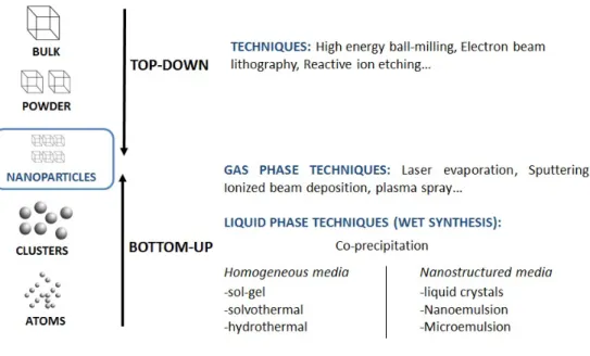
(12) 1.1. Introduction. Nanostructured materials possess at least one dimension in the nanometer scale (10−9 m). The high interest in nanomaterials observed in recent years is mainly due to the quantum size effects leading to interesting changes in various properties. Few examples are listed below:. • Optical: the color of noble metal nanoparticles is found to depend on the shape and size of the nanoparticle and dielectric constant of the medium so a dispersion of gold nanoparticles can have several colors going from red to black.. • Magnetic: Superparamagnetic behavior is observed for nanoparticles whereas the corresponding bulk materials possess ferromagnetic behavior.. In order to explore novel physical properties and phenomena of nanostructured materials, the ability to synthesize these materials in a controlled manner is the first and most important step. The general strategies for the preparation of nanomaterials can be classified as Top-down and Bottom-up (Figure 1.1).. A typical top-down approach consists of using mechanical attrition in order to reduce from the bulk size to the nanosize. Various techniques are employed such as high energy ball-milling [4], electron beam lithography [5], reactive ion etching [6] and so on. On the contrary, the bottom-up strategies are based on the physicochemical principles of molecular or atomic self-organization. From atoms or molecules, clusters are formed promoting nanoparticle formation.. By the bottom-up strategy, two types of approach are used: gas phase and liquid phase techniques. Gas phase techniques include laser evaporation [7], sputtering [8], ionized beam deposition [9], plasma spray [10] and so on. 12.

(13) Figure 1.1: Methods of nanoparticle preparation: Top-down and Bottom-up strategies.. Concerning the liquid phase techniques, these can be in homogeneous (solution) media such as sol-gel [11], hydrothermal [12], co precipitation, [13] solvothermal; or it can be in a nanostructured media such as in microemulsions [14–17] among others. The microemulsion reaction method is one of the most used techniques for the preparation of very small and nearly monodispersed nanoparticles. This method offers a series of advantages with respect to other methods, namely, the use of simple equipment, the possibility to prepare a great variety of materials with high degree of particle size and composition control, the formation of nanoparticles with often crystalline structure and high specific surface area, plus the use of soft conditions of synthesis, near ambient temperature and pressure. The traditional method is based on water-in-oil microemulsions (W/O), and it has been used for the preparation of metallic and other inorganic nanoparticles since the beginning of the 1980s. [14] Since the discovery of microemulsions, the literature in this topic has grown steadily and there are reviews about different aspects of the method such as; reactivity, mechanism, control of particle size and shape, etc. [15, 18–23]. 13.

(14) These studies provide insightful information regarding the use of W/O microemulsion as reaction media for the synthesis of inorganic nanoparticles. However, research in this field is still short on information regarding the mechanism of formation and growth of the final nanoparticles. Based on some disadvantages of the W/O microemulsion reaction method, such as the use of large amount of organic solvent, a method based on O/W microemulsion as confined reaction media was developed. [24] This method consists of the use of organometallic precursors, dissolved in nanometer scale oil droplets stabilized by a monolayer of hydrophilic surfactant. The precipitating agents, usually water soluble, can be added directly or as aqueous solutions, without compromising microemulsion stability and droplet size. There have been a number of advances in different aspects of the synthesis of nanoparticles in microemulsions, such as: the use of other types of microemulsions (O/W and bicontinuous) for synthesis, preparation of more complexes structures, synthesis of more complex ceramics, modeling of reactions in microemulsions. Still, there is a lack of information regarding the detailed structure of the microemulsions used for the synthesis of nanomaterials, in particular with O/W microemulsions. This can be done with the use of techniques such as: Dynamic Light Scattering (DLS) and Small Angle Neutron Scattering (SANS). [17, 25] Most of the experimental and theoretical work published up to date regarding the synthesis of inorganic nanoparticles in microemulsions has been devoted to study the use of W/O microemulsion systems. [15, 21, 26–28] Regarding synthesis in O/W microemulsions, the literature is focused on the synthesized particles themselves without going into detail in the characterization of the microemulsions used for synthesis or the kinetics or mechanistic aspects of the synthesis. [24, 29, 30] A better understanding of the system dynamics and characteristics can lead to a better description of the O/W microemulsion reaction method as it has not been studied in detail. In the present work, the method of choice for the preparation of inorganic nanoparticles is the oil-in-water microemulsions reaction method. This approach has shown versatility and control in particle size, as well as the morphology, homogeneity and 14.

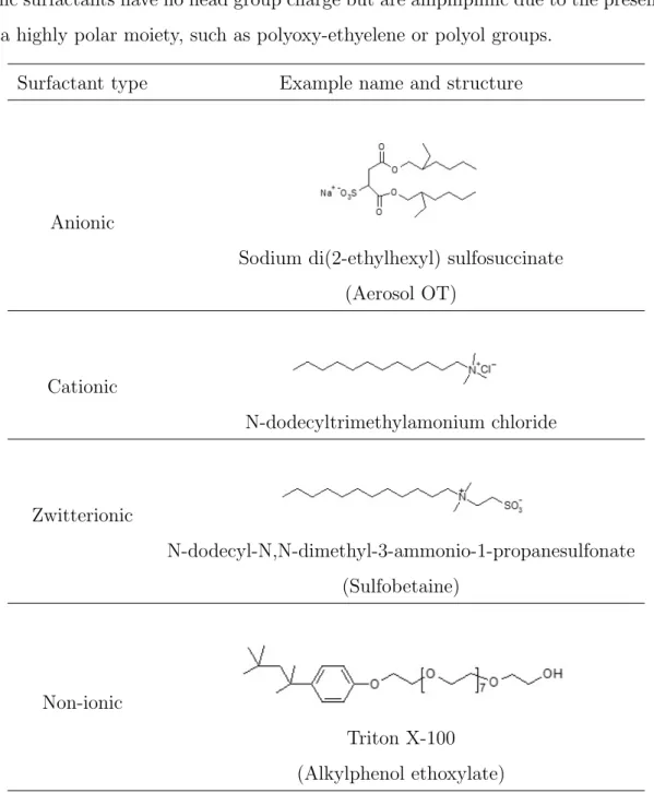
(15) surface area of the materials obtained; however, nothing is known about the characteristics of the O/W microemulsions used for synthesis or the kinetics and mechanisms involved. [24]. 1.2 1.2.1. General Theoretical Background Colloids. Colloids are ubiquitous in nature and in a broad range of scientific and technological areas. These systems consist of one substance finely dispersed in another. Particles that are in size range approximately between 1 µm down to 1 nm in size are classified as colloidal particles. [31] A major group of colloidal systems are called association colloids [32] which contain amphiphilic (affinity to both water and oil) molecules that associate in a dynamic and thermodynamically driven process to produce aggregates that are a molecular solution and a colloidal system. Such molecules are commonly termed surfactants.. 1.2.2. Surfactants. The term surfactant is a contraction of surface-active agent. As their name suggests, surface-active agents are organic molecules that, when dissolved in a solvent, have the ability to self-assembled and adsorb at interfaces (whether liquid/liquid interface, liquid/air or even solid/liquid) in an oriented manner. Adsorption occurs due to the nature of the solvent and the chemical structure of surfactants, which posses a polar part (the ”‘head group”’) and a non-polar part (the ”‘tail”’).. Surfactant classification There are many possible variations within the structure of surfactants, therefore different types of classification. Since the hydrophilic part normally achieves its solubility either by ionic interactions or by hydrogen bonding, surfactants can be broadly classified into four categories based on the nature of the surfactant head 15.

(16) group type (Table 1.1). Anionic surfactants have negatively charged head groups such as alkyl phosphates or sulfates (e.g. sodium dodecyl sulfate). Cationic surfactants have positively charged head groups and are usually based on quaternary ammonium compounds (e.g. dodecyltrimethyl-ammonium bromide). Zwitterionic or amphotherics, are surfactants which combine both a positive and negative groups and are often biologically important (e.g. Cocamidopropyl betaine). Finally, nonionic surfactants have no head group charge but are amphiphilic due to the presence of a highly polar moiety, such as polyoxy-ethyelene or polyol groups. Surfactant type. Example name and structure. Anionic Sodium di(2-ethylhexyl) sulfosuccinate (Aerosol OT). Cationic N-dodecyltrimethylamonium chloride. Zwitterionic N-dodecyl-N,N-dimethyl-3-ammonio-1-propanesulfonate (Sulfobetaine). Non-ionic Triton X-100 (Alkylphenol ethoxylate) Table 1.1: Examples of some common surfactants molecules according to their head group classification.. Differences in the nature of the hydrophobic group are usually less pronounced 16.

(17) than those for the hydrophilic group. The most common groups are long-chain hydrocarbons. Nevertheless, they include different structures such as: • Straight chain alkyl groups (C8 − C20 ) • Branched-chain, long alkyl groups (C8 − C20 ) • Long chain (C8 − C20 ) alkylbenzenes • High molecular weight propylene oxide polymers • Perfluroalkyl groups • Polysiloxane groups Finally, new surfactant molecules have recently emerged with interesting or enhanced properties, thus the best option for their classification is according to the structural features of the molecules. These novel surfactants include catanionics, bolaforms, gemini surfactants, polymeric and polymerizable surfactans,etc. (Figure 1.2).. Figure 1.2: Some examples of functionalized surfactants. 17.

(18) Non-ionic surfactants. As mentioned above, non-ionic surfactants are amphiphilic molecules with an uncharged headgroup. Most non-ionic surfactants bear ethylene oxide chains as the polar part, and the most common are the fatty alcohol ethoxylated surfactants. The polar hydrophilic group of non-ionic surfactants dissolves in water through hydrogen bonding. As this is a temperature-sensitive interaction, non-ionic surfactants often exhibit inverse temperature solubility. Therefore, an important characteristic of micellar solutions of non-ionic surfactants is that, at a certain critical temperature (Cloud point), they become visibly turbid. [32–35] This effect depends on the chemical structure of the surfactant, making their activity as emulsifiers and stabilizers temperature-sensitive. Other types of non-ionic surfactants are: sorbitan esters and alkylpolyglucosides (sugar derivatives), fatty alkanolamides, oxyethylated fats and oils, amine oxides, long chain carboxylic acid esters and N-alkyl pyrrolidones are also included. The lack of charge in non-ionic surfactants makes them compatible with other types of surfactants and, in general, are resistant to high concentration of electrolytes. One important characteristic of non-ionic surfactants is the possibility of relating quantitatively their polar and apolar groups by an empirical equation, denoted as the Hydrophilic Lipophilic Balance (HLB) number. This concept was introduced by Griffin [36, 37].. HLB =. Ej wt% + OHwt% 5. (1.1). where Ej wt% and OHwt% are the weight percent of ethylene oxide and hydroxide groups, respectively. Later, Davies [38] developed a more global method to calculate the HLB number from chemical formulas of surfactants, using empirically determined group members.. HLB = [(nH · H) − (nL · L)] + 7 18. (1.2).

(19) Where H and L are the hydrophilic and lipophilic groups constants, respectively, while nH and nL are the number of these groups per surfactant molecule. In general, HLB number increases indirectly with the global polarity of the molecule (number of etoxylated units), and it can be used in order to determine the capacity of certain surfactant for specific purposes. Griffin’s HLB number is widely used, but the effect of a surfactant concentration, an oil/water ratio, and temperature on emulsion type and stability is not accounted for in his calculation.. 1.2.3. Microemulsions. Microemulsions are single phase, optically isotropic, fluid and thermodynamically stable liquid solutions formed by the mixtures of two immiscible liquids and surfactant (and sometimes with the addition of a co-surfactant) that form spontaneously. [31, 39, 40] Microemulsion droplets are usually in the size range of 2 − 50 nm in radius (much smaller that emulsion droplets, > 0.20 µm). The formation of a microemulsion depends mainly on the surfactant type and structure, as well as the oil/surfactant ratio, temperature and salinity. Once the conditions are adequate, this results in one of the fundamental properties of microemulsions, that is, lowering the interfacial tension between the oil and water phases to ultralow values (10−2 −10−3 mN m−1 ), so that spontaneous dispersion of water or oil droplets occurs and the system reaches thermodynamic stability.. Three types of microemulsion structures exits; nanometer-size oil droplets stabilized by a monolayer of surfactant dispersed in water are called oil-in-water (O/W) microemulsions; the reverse system called water-in-oil (W/O) microemulsion consists of nanometric size water droplets stabilized by a surfactant monolayer and dispersed in a continuous oil-phase, and finally the bicontinuous microemulsions, in which both oil and water form continuous domains as interconnected sponge-like channels. (Figure 1.3) 19.

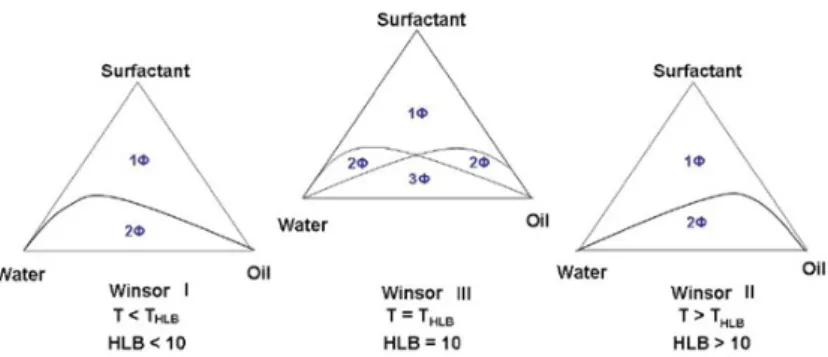
(20) Figure 1.3: Types of microemulsion: oil-in-water microemulsion, bicontinuous microemulsion, and water-in-oil microemulsions.. In 1948, Winsor classified microemulsions into four main types of equilibria (figure 1.4). [41] Type 1: The surfactant is preferentially solubilized in water and O/W microemulsions form. Surfactant-rich water phase co-exists with the excess oil phase where surfactant is only present as monomers at small concentration (Winsor I). Type 2: The surfactant is preferentially dissolved in the oil phase and W/O microemulsions form. Surfactant-rich oil phase co-exists with the surfactant-poor aqueous phase (Winsor II). Type 3: A three-phase system where a surfactant-rich, middle-phase (bicontinuous) microemulsion co-exists in thermodynamic equilibrium with both excess oil and water phases (Winsor III). Type 4: A single-phase (isotropic) micellar solution forms upon the addition of a sufficient quantity of amphiphile. This microemulsion may be O/W, W/O or bicontinuous.. Figure 1.4: Classification of microemulsions. In the three phase system the middlephase microemulsion (BC ME) is in equilibrium with both excess oil (O) and water (W).. Depending on the surfactant nature and the conditions (composition, surfactant/oil 20.

(21) ratio, temperature, addition of solutes), the different Winsor types of microemulsions will be selectively formed. Certainly, the formation of these systems depends on the molecular arrangement at the oil-water interface. Nevertheless, this molecular arrangement is also sensitive to other variables that can promote phase transitions, such as the incorporation of electrolytes in the presence of ionic surfactants or temperature change with non-ionic surfactants.. 1.2.4. Phase behavior of Water/Non-ionic Surfactant/Oil systems. As mentioned above, the properties of non-ionic surfactant systems are highly sensitive to temperature changes. The maximum solubilisation of both aqueous and oil phases is achieved at a critical temperature where the hydrophilic and liphophilic properties of the system are balanced. This temperature is dependent on the composition of the system, and it is denoted as the Hydrophilic-Lipophilic Balanced Temperature (TH LB ).1001[42, 43] The Winsor phase equilibria explained previously can be described in a ternary phase diagram (Figure 1.5). At constant temperature and pressure, the ternary phase diagram of a simple three component microemulsion is divided into two or four regions: [44, 45]. Figure 1.5: Ternary phase diagram representation of Winsor type equilibria for nonionic surfactant systems at different temperatures.. The region containing two phases (2φ) comprises a microemulsion in thermodynamic equilibrium with an excess phase, which can be either water or oil. Winsor I pro21.

(22) motes the formation of O/W microemulsion in thermodynamic equilibrium with an excess oil phase. Winsor II gives rise to the formation of a W/O microemulsion in equilibrium with an excess aqueous phase. At the temperature TH LB , a region with three liquid phases in equilibria appears, which are an aqueous phase constituted by surfactant in submicellar concentration, water, an oil phase and a bicontinuous microemulsion. This phase equilibria is called Winsor III. The transition Winsor I > III > II is accomplished by increasing the temperature. This temperature depends on the composition of the system, thus, if reagents (precursors or precipitating agents) are added, TH LB may be shifted. In non-ionic surfactant-based microemulsion, a strong influence of the presence of solutes on the phase behavior has been observed. [17]. 1.2.5. Microemulsion as reaction media for the synthesis of inorganic nanoparticles. The use of microemulsions as confined reaction media represents a soft and straightforward alternative to the generation of nanomaterials. [24] Microemulsions may occur in the form of water-in-oil (W/O) and oil-in-water (O/W) droplets, as well as bicontinuous structures. Their used as reaction media for the synthesis of inorganic nanoparticles has been developed and explored further.. 1.2.6. The Water-in-Oil microemulsion reaction method (W/O). The use of W/O microemulsions for the synthesis of inorganic nanoparticles was first reported in 1982. [14] The droplets of W/O microemulsions are conceived as tiny compartments or ”‘nanoreactors”’. The main strategy for the synthesis of nanoparticles in W/O microemulsions consists in mixing two microemulsions, one containing the metallic precursor and another one the precipitating agent. Upon mixing, both reactants will contact each other due to droplet collisions and coalescence, and will react to form precipitates of nanometric size (Figure 1.6), which may remain confined to the interior of microemulsion droplets or they may remain stabilized by 22.

(23) surfactant molecules in the continuous oil phase. Examples of the great variety of nanomaterials that have been synthesized by this method include: metallic and bimetallic nanoparticles, single metal oxide as well as mixed metal oxides, quantum dots, core-shell structures, and even complex ceramic materials such as spinels and perovskites. [15, 18–23]. Figure 1.6: Schematic representation of the W/O microemulsion reaction method for the synthesis of inorganic nanoparticles.. It has been reported that materials synthesized in W/O microemulsions exhibit unique surface properties; for example, nano-catalysts prepared by this method show better performance (activity, selectivity) than those prepared by other methods. [23] The method offers a series of advantages with respect to others (co-precipitation in solution [46], sol-gel [46], flame spray pyrolysis [47], laser evaporation, high energy milling, etc); namely, the use of uncomplicated equipment, homogeneous mixing, the possibility to prepare a great variety of materials with a high degree of particle size and composition control, the formation of nanoparticles with often crystalline structure and high specific surface area, and the use of soft conditions of synthesis, near ambient temperature and pressure. But in spite of the superior properties and performance of nanoparticles obtained in W/O microemulsions, this method has not found good acceptance at the industrial level, mainly due to the employment of large amounts of oils (solvents), which represent the continuous phase and hence the main component of these systems [23]. In addition, most studies employ relatively low concentration of the metal precursors, leading to small yields of nanoparticles per microemulsion volume. These drawbacks affect negatively from the economic and ecologic point of view. 23.

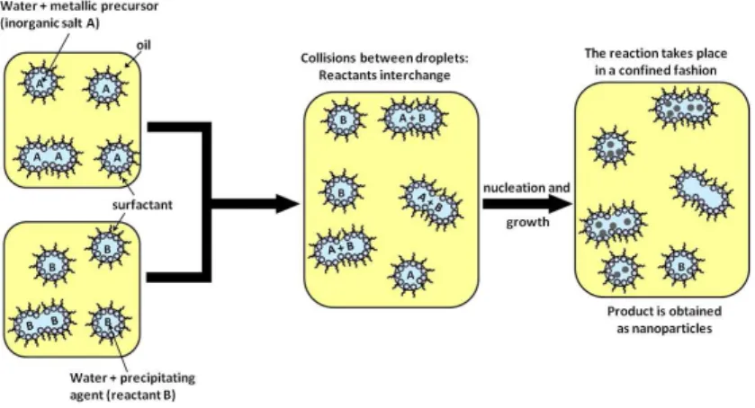
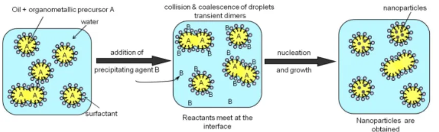
(24) 1.2.7. The Oil-in-Water microemulsion reaction method (O/W). Based on the disadvantages of the classic W/O microemulsion reaction method mentioned above, a method based on O/W microemulsions as confined reaction media was recently developed for the preparation of metallic and metal oxide nanoparticles. [24] This method consists of the use of organometallic precursors, dissolved in nanometer scale oil droplets stabilized by a monolayer of hydrophilic surfactant as shown in Figure 1.7. The precipitating agents, usually water soluble, can be added directly or as aqueous solutions, without compromising microemulsion stability and droplet size; alternatively, if oil-soluble precipitating agents are available, then a two microemulsions approach can be used. The main advantage of this new approach is the use of water as a continuous phase, more environmentally friendly than organic solvents generally used in the traditional W/O microemulsion method. [24, 29, 30] As it has been described, most of the experimental and theoretical work published up to date regarding the synthesis of inorganic nanoparticles in microemulsions has been devoted to study the use of W/O microemulsion systems. [15, 21, 26, 28, 48] Regarding synthesis in O/W microemulsions, the literature is focused on the synthesized particles themselves without going into detail in the characterization of the microemulsions used or the kinetics or mechanistic aspects of the synthesis. [24, 29, 30] A better understanding of the system dynamics can lead to a better description of the O/W microemulsion reaction method as it has not been studied in detail.. Figure 1.7: Schematic representation of the O/W microemulsion reaction method for the synthesis of inorganic nanoparticles.. The first work reported as a proof of concept was the synthesis of metallic (Pt, Pd, and Rh) as well as metal oxide (CeO2 ) nanoparticles [24]. The synthesis of 24.

(25) mesoporous mixed oxides has also been reported (CeO2 , ZrO2 , Ce0.5 Zr0.5 O2 and T iO2 ) with high specific surface area, between 200-380 m2 g −1 . [29] Is important to highlight that all synthesis were carried out under soft conditions (around 20◦ C). These materials were evaluated as catalyst supports; all of the materials showed a good activity in CO oxidation at low temperature. These studies demonstrates the feasibility of this approach for the preparation of highly active catalysts. Magnetic nanoparticles (iron oxide) have also been synthesized using W/O and O/W microemulsions. Iron oxide nanoparticles were obtained with sizes ranging from 2-10 nm and their potential application for protein binding/protein purification was investigated and compared. Magnetic nanoparticles prepared from O/W microemulsion method showed larger surface area and porosity and smaller size (3 nm). [49] Cobalt nanostructures with different size and morphology has also been synthesized by the W/O and O/W microemulsions. Influence of the surfactant and precipitating agent was investigated. The final shape and size of cobalt nanostructures were controlled by changing the type of reaction media as well as the precipitating agent. Moreover, the use of O/W microemulsion generated better results in terms of colloidal stability and uniformity of particle size with respect to W/O microemulsion. [50]. Mechanism of nanoparticle formation in microemulsions A model of particle precipitation in a homogeneous aqueous medium has been proposed by La Mer. [1] The model involves particle nucleation at short times. As soon as monomer formation takes place due to chemical reaction, its concentration increases up to the point of spontaneous nucleation, which occurs over a critical supersaturation concentration [C]C . Afterwards, growth takes place (Figure 1.8). The growing step is mainly controlled by the diffusion of monomers in solution (C) onto the particles surface. Thus, C reaches a maximum and afterwards it begins to decrease. This decrease in monomer concentration is due to the growth of the particles by diffusion. In microemulsions, the number of nucleated sites is expected to be higher, comparing to homogeneous reactions, as illustrated in Figure 1.8. On 25.

(26) the other hand, the diffusion controlled particle growth should occur at lower rate. Another model is based on the thermodynamic stabilization of the particles. In this model the particles are thermodynamically stabilized by the surfactant. The size of the particles remains constant when the precursor concentration and the size of the aqueous droplets vary. Nucleation occurs continuously during the nanoparticle formation, this might be the case in the O/W microemulsions.. Figure 1.8: Monomer concentration [C] as a function of time in microemulsions, compared to a homogeneous system. [1]. Reaction kinetics Although W/O microemulsions as reaction media for the synthesis of inorganic nanoparticles have been extensively studied, the kinetics of these reactions is still not completely understood. As mentioned above, several types of nanoparticles have been synthesized using a variety of surfactant systems, and relationships between the nanoparticles characteristics and the microemulsion media are not straightforward due to the diversity of variables which can have an influence, and this may be closely related with complex kinetics. An effort to relate the surfactant media with the reaction kinetics was reviewed by Lopez-Quintela et al. [51], concerning both inorganic and organic syntheses in microemulsions. Only a few studies can be cited concerning the follow-up of reactions with time, due to the fast rate of W/O microemulsion reactions. Bandyopadhyaya et al. [52] have modeled CaCO3 formation in microemulsions by carbonation. A time-scale analysis was developed, resulting in a model of reaction kinetics that closely corresponded to results obtained experimentally. 26.

(27) Chew et al. [53] have studied the effect of alkanes in the formation of AgBr particles in ionic W/O microemulsions (using AOT as surfactant), where the transmittance of the reactions were followed with time with UV-Vis and Stopped-Flow Spectrophotometry. They have found an increase on reaction rate with the chain length of the alkane. Curri et al. [54] studied the role of cosurfactant on the synthesis of CdS nanoclusters, using CTAB as surfactant. Stopped-Flow Spectrophotometry was used in order to compare a reaction using CTAB plus cosurfactant and other carried out using AOT. They have summarized two different cosurfactant effects: the influence of the surfactant film flexibility on particle growth and the particles stabilization in solution, determined by the adsorption of cosurfactant onto the particle surface. Lopez-Quintela et al. [28] simulated the kinetics of nanoparticles formation in microemulsions. Simulations were carried out by comparing Ag, Ag-Au and Au formation with experimental data reported by Destre and Nagy. [21] C. Tojo et al. developed a Monte Carlo simulation model, in which predicts the metal distribution in bimetallic nanoparticles (Au/Pt and Au/Ag) and allowed them to study nanoparticle formation from kinetic point of view. The final composition of the nanoparticle was controlled by changing the initial reactant concentration inside the micelles. [55] The detailed comprehension of the kinetics taking place in microemulsion reactions is limited by the experimental data in this direction. Hence, systematic studies focused on reaction rates are greatly encouraged in order to advance in this field.. Parameters influencing nanoparticle synthesis in microemulsions Although complete control of particle characteristics is still far from clear and direct, some trends can be pointed out as shown below. It have been described in several publications the particle size dependency with water:surfactant molar ratio (w0 ) in W/O microemulsions. In general, it has been observed that, as increasing w0 , an increase on particle size is observed. [15, 19] However, Cason et al. [56] have found that, with different w0 , it was possible to 27.

(28) obtain constant particle size if the reaction time increases for the synthesis to get completed. They proposed that the growth of the particles is affected by w0 . It was considered that for low w0 values, the aqueous solution is not enough to completely hydrate the polar groups of the surfactant and the counterion. As a consequence, the film rigidity is higher compared to higher w0 values. This influences on the micellar exchange and, as a consequence, the growth rate decreases. Increasing w0 , the micelle rigidity decreases generating an increase in the growth rate up to a certain concentration, where further increase in w0 simply causes reagent dilution, which causes a decrease in the growth rate. Some studies have indicated a decrease on particle size with w0 [57]. Particle size have been determined to be directly dependent on reagent concentration. [15] An example is the work carried out by Destre and Nagy. [21] They have synthesized Pt nanoparticles, using different concentrations of K2 P tCl4 . An increase on particle diameter from 2 to 12 nm was obtained, by increasing the concentration of the precursor. On the other hand, an increase on the precipitating precursor ratio generally causes a decrease on particle size. [58] It is thought that increasing precipitating agent concentration, particle nucleation can be favored to a higher extent, which further grow simultaneously, resulting in particles with lower size and polydispersity. The effect of surfactant chainlength and cosurfactant addition has been studied. As the lipophilic chain of the surfactant is longer, smaller particles are obtained due to the increased micellar rigidity. Generally, the addition of cosurfactant causes an increased micellar exchange, due to the decrease in the interfacial film rigidity. It is thought that the increase in microemulsion droplet size is counteracted with the increase on surfactant film curvature, generating smaller particles than without cosurfactant. [51] Some studies have shown that low weight oil molecules, with low molecular volumes, can penetrate in the surfactant hydrocarbon chains, increasing the film curvature and rigidity. [56] This effect has been observed to produce micellar exchange decrease and, consequently, smaller particles are obtained. Some studies reveal the possible dependence of nanoparticle shape with electrolyte 28.

(29) addition. [59] Pileni [18] has postulated that the selective ion or molecule adsorption over nanocrystal layers can affect their growth in certain directions, which could explain the apparent preference on certain particle shape. As it has been observed, there are many parameters and reaction conditions that can influence the characteristics of nanoparticles synthesized using microemulsions as reaction media. After more than 30 years of the use of W/O microemulsions as confined reaction media for the synthesis of inorganic nanoparticles, it is clear that understanding the mechanism of nanoparticles formation is quite complicated and far from being completely understood. Furthermore, the advantages offered by newly developed methods such as the O/W and bicontinuous microemulsion methods, highlight the need to understand these methods as well. In particular, the O/W microemulsion method has demonstrated its usefulness for the synthesis of a large variety of materials. For all these reasons, the focus of this thesis is to set the basis for understanding these systems, in order to further improve the reach of the methods. This is done from two perspectives: the characterization of the microemulsions used for synthesis (SANS, DLS, conductivity), as well as preliminary studies of reaction kinetics and mechanisms. These type of studies are carried out for the first time for O/W microemulsions used for the synthesis of inorganic nanoparticles.. 29.

(30) Chapter 2 Aims. 30.

(31) The use of water-in-oil microemulsions as reaction media for the synthesis of inorganic nanoparticles is widely known. The more recent, oil-in-water microemulsion method has proof to have a lot of advantages over the previous methods, and all the reported synthesis in oil-in-water techniques focus on the synthesized materials and their properties. However, the main synthetic characteristics about this method are not fully elucidated. So far, it has only been suggested that there has to be an interfacial mechanism using precursors of type 2-ethylhexanoate. This project contemplates the study of the synthesis of different inorganic nanoparticles (metallic and metal oxide) by this technique, characterizing the molecular structure of the microemulsions with different types of precursors. By understanding the mechanism of formation of nanoparticles in oil-in-water microemulsion reactions and the relationship between the obtained material and microemulsion composition, this promise a more sophisticated approach to control and manipulate the synthesis of nanoparticles, with economic and environmental implications for reducing surfactant usage, waste and potentially affording low energy impact.. 2.1. Hypothesis. Precursors with different molecular structure have different mechanisms of formation of inorganic nanoparticles in oil-in-water microemulsions as reaction media. Precursors of type metal 2-ethylhexanoate are located mainly at the oil-water interface with the surfactant, whereas, the type of precursors (1,5-cyclooctadiene)dimethyl metal are located inside the droplet. Consequently, the first precursors have an interfacial mechanism while the second gives way to a mechanism controlled predominantly by micellar interchange and droplet collisions.. 2.2. Aims. The main purpose of this project is to study the fundamental aspects of reactions carried out in oil-in-water microemulsions as reaction media, for the synthesis of various inorganic nanoparticles from organometallic precursors and the investiga31.

(32) tion of the relationship between the microemulsion properties and the obtained nanoparticles characteristics.. The specific objectives of this investigation are described below: • Design of. O. /W microemulsion systems using different types of metalorganic. and organometallic precursors, dissolved in the internal oil phase, such as: Cerium (III) 2-ethylhexanoate, Copper (II) 2-ethylhexanoate and (1,5cyclooctadiene)dimethylplatinum (II). • Characterization of the microemulsion type through conductivity measurements. • Characterization of the microemulsions:. determination of hydrodynamic. droplet size with Dynamic Light Scattering. • Characterization of the systems through SANS (Small Angle Neutron Scattering) to determine structure, morphology, size and interactions in the O /W microemulsion systems. • Synthesis and characterization of various types of inorganic nanoparticles (CeO2 , CuO and Pt) by the O /W microemulsion reaction method. • Preliminary kinetic studies followed by UV-Vis spectroscopy as a function of time of nanoparticles synthesized by the O /W microemulsion method. • Preliminary kinetic study followed by High Resolution Transmission Electron Microscopy (HR-TEM).. 32.

(33) Chapter 3 Experimental Part. 33.

(34) 3.1 3.1.1. Materials Surfactants. For the development of this project non ionic surfactants were used without further purification. These surfactants are ethoxylated primary alcohols with full saturation.. Synperonic. 91. /5 , (CH3 (CH2 )9 (OC2 H4 )5 OH), HLB=12, Cloud point 36◦ C, from. Croda. Commercial non-ionic surfactant C10 E5 , this formula indicates the average chain length, since commercial surfactants contain a mixture of chain lengths; this particular surfactant has a hydrocarbonated chain with an average of 10 carbon atoms, whilst the ethylene oxide chain has an average of 5 ethylene oxide units. The hydrocarbon chain from this surfactant is linear and fully saturated.. Brij O10 C18 H35 (OCH2 CH2 )n OH, n 10, HLB = 12.4, Cloud point <50. ◦. C, from. Sigma Aldrich. This non-ionic surfactant has an alkyl length chain of 18 carbon atoms and an ethylene oxide chain with an average of 10 units, the hydrocarbon chain is not fully saturated.. 3.1.2. Aqueous components. Water was Millipore grade with a resistivity of 18.2 M Ω· cm at 25 ◦ C and for the case of SANS experiments D2 O obtained from Eurisotop (99.9% D) was employed.. 3.1.3. Oils. Isooctane or 2, 2, 4-trimethylpentane (C8 H18 ) (Chromasolv Plus for HPLC >99.5%) from Sigma Aldrich, Mw 114.23 g /mol , ρ 0.692 g /mL , and nD20 1.391. Butyl (S)-(-)-Lactate CH3 CH(OH)COO(CH2 )3 CH3 , >97%, from Sigma Aldrich, Mw 146.18 g /mol , ρ 0.984 g /mL , and nD20 1.394.. 34.

(35) 3.1.4. Metalorganic/Organometallic Precursors. (1,5-cyclooctadiene) dimethylplatinum (II) C10 H18 P t 97%, from Sigma Aldrich, Mw 333.33 g /mol , %Pt 56% according to the certificate of analysis (Sigma Aldrich) of batch MKBN2971V.. Cerium (III) 2-ethylhexanoate, 49% in 2-ethylhexanoic acid, C24 H45 CeO6 from Alfa Aesar, Mw 569.74 g /mol , ρ 1.08 g /mL , %Ce 12.08 (determined by ICP).. Copper (II) 2-ethylhexanoate, C16 H30 CuO4 Alfa Aesar, Mw 349.96 g /mol , %Cu 18.07% (according to the certificate of analysis (Alfa Aesar) of Batch J10X027).. 3.1.5. Precipitating agents. Tetramethyl. ammonium. hydroxide. pentahydrate. (TMAH,98%). (CH3 )4 N (OH)5H2 O- from Sigma Aldrich, Mw 181.23 g /mol . Ammonium hydroxide solution 28-30% N H4 OH - from Sigma Aldrich, Mw 35.05 g. /mol .. Sodium borohydride 99.99% (N aBH4 ) - from Sigma Aldrich, Mw 37.83 g /mol . Ascorbic acid 6-palmitate C22 H38 O7 - from Sigma Aldrich, Mw 414.53 g /mol . Sodium hydroxide anh. pellets >98% - from Sigma Aldrich, Mw 40.00 g /mol . Curcumin [HOC6 H3 (OCH3 )CH = CHCO]2 CH2 - from Sigma Aldrich, Mw 368.38 g. /mol .. 3.2 3.2.1. Techniques Specific electrical conductivity. Conductivity is the ability of a material to conduct electric current and a typical conductivity meter will apply an alternating current (I) between two electrodes and 35.

(36) it will measure the potential (V) and by the Ohm Law the electrical conductivity can be calculated (equation 3.1).. R=. V I. (3.1). Where V is the voltage in volts, I is the current in Amperes and R is the solution resistivity in MΩ and the conductance is defined as the reciprocal of the electrical resistance of a solution between two electrodes, G =. 1 . R. The units of electrical. conductivity are the Siemens (S).The conductivity meter then uses the conductance and cell constant to display the specific electrical conductivity in (S/cm or µS/cm or mS/cm). Conductivity experiments were carried out using a Thermo Scientific Orion Star A212 Conductivity Benchtop Meter. The conductivity cell model was Orion DuraProbe 4-electrode conductivity cell with graphite sensors, and a nominal cell constant of 0.475 cm−1 . The samples were placed in a vial with just one inlet for the conductimeter cell as showed in Figure 3.1. The samples were cooled around 5◦ C in a thermostated bath, and the temperature was slowly increased up to 60◦ C and the electrical conductivity measurements were recorded as a function of temperature every 0.2◦ C. Strong magnetic stirring was applied during the measurements in order to obtain permanently an homogeneous sample. The temperature increase was carried out slowly in order to allow the sample to reach microemulsion phase changes.. Figure 3.1: Set up for the conductivity experiments. 36.

(37) 3.2.2. Dynamic Light Scattering (DLS). Dynamic Light Scattering (DLS) is also known as Photon Correlation Spectroscopy (PCS). This technique is a very well known, non invasive technique used for the determination of the hydrodynamic radius of colloidal systems. This technique is based on the detection of the fluctuations of the scattered light with time at a certain scattering angle (Figure 3.2). Due to the relation of the Brownian motion of the particles caused by thermal fluctuations in the media.. Figure 3.2: Schematic representation of the conventional Dynamic Light Scattering instrument with a goniometer.. In order to quantify the mobility of the particles by light scattering the scattering intensity fluctuation is expressed in terms of a correlation function, and from here it can be obtained not only of the diffusivity of the particles but also their size. For a suspension of monodisperse, spherical particles undergoing Brownian diffusion, the autocorrelation function decays exponentially with the delay time and it is given as. 2. g 1 (τ ) = A · e−Dq + B. (3.2). where A is the amplitude of the correlation function, B is the baseline, D is the translational diffusion coefficient of the particles, and q is the magnitude of the scattering vector defined as 37.

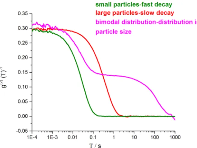
(38) q=. θ 4πn sin λ0 2. (3.3). Here, n is the refractive index of the medium. For spherical particles, the hydrodynamic radius Rh can be obtained from the translational diffusion coefficient (D) using the Stokes-Einstein relationship. D=. kT 6πηRh. (3.4). where k is the Boltzmann constant, η is the solvent viscosity, and T is the absolute temperature. If the particle is nonspherical, then Rh is often taken as the apparent hydrodynamic radius or equivalent sphere radius.. Dynamic Light Scattering measurements were performed in the compact ALV/CGS3 instrument equipped with a He-Ne laser with a wavelength of λ=632.8 nm. Pseudocross-correlation functions were recorded using an ALV 5000/E multiple-τ correlator at scattering angles θ from 50 to 120◦ set with an ALV-SP 125 goniometer. All measurements were carried out at 25 ◦ C in a thermostatted toluene bath. (3.3). Figure 3.3: DLS instrument model ALV/CGS-3. From simple observation of the correlogram graph from a DLS experiment one can obtain a lot of information about the sample. The time at which the correlation starts to significantly decay is an indication of the mean size of the sample. The steeper the line, the more monodisperse the sample is. Quite opposite, the more extended the decay becomes, the greater the sample polydispersity. Or when a bimodal distribution is observed this could be due to polydispersity present in the sample or due to interactions in the sample.(Figure 3.4) 38.

(39) Figure 3.4: Autocorrelation function recorded for different samples for purposes of comparison (size and decay rates).. 3.2.3. Kinetics followed by UV-Vis Spectroscopy. UV-visible radiations stimulate molecular vibrations and electronic transitions. By this technique, the transmittance or absorbance values are plotted as a function of wavelength (nm). This method is relevant for the identification of organic and many inorganic species. Also it is widely used for kinetic studies which involve the measurement of the change in concentration of a certain reactant or product of a reaction as a function of time, this can be followed at a fixed wavelength. Two different models of Spectrophotometer from Agilent Technologies were used (Cary 50 and Cary 5000 UV-Vis Spectrophotometers). The absorption spectroscopy was recorded from 160 to 780 nm at room temperature (25◦ C). The evolution of the formation of CeO2 and P t nanoparticles was investigated separately by means of UV-Vis experiments. The structural and optical information acquired corresponded to the firsts minutes of the reactions with a dead time of approximately of 1.5 minutes. Several tests were carried out, in which composition of the microemulsion was selected as well as the precursor concentration and precipitating agent. The type of observation cell used was a quartz cuvette with a path length of 1 mm. The evolution of spectra was followed until the stabilization of the absorbance (approximately 1h after reaction started). The experiment was focused on the determination of the optimum wavelength and optimum reaction conditions for further kinetic studies. 39.

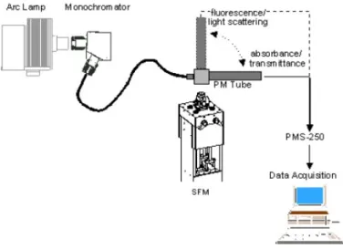
(40) 3.2.4. Stopped Flow Technique (SF). Kinetic studies were also carried out by absorbance measurements as a function of time with a monochromator spectrometer MOS (BioLogic) connected to an stoppedflow device (SFM-400). A schematic representation of the configuration can be observed in Figure 3.5. Figure 3.5: Schematic representation of the configuration used for kinetic studies. Figure 3.6: Schematic representation of the configuration of Stopped Flow equipment SFM 400. The stopped-flow sub-system consists of four independent stepping-motors syringes, one valve is blocked and there is a possibility to include one to three mixers (Figure 3.6). All the valves, delay lines and the cuvette are enclosed in a water jacket to allow temperature regulation of the reactant containers. A Xe(Hg) light source 40.

(41) was used for illumination of the sample. Connection to the stopped-flow cuvette is done through a fiber optic cable. Millisecond dead time can be achieved with the equipment due to the combined effects of stepping motors control and low dead volumes. The motor power supply unit contains independent constant current power supplies for each syringe, all driven independently by their own microprocessor. The Stopped-Flow module is controlled by Bio-Kine software. Two to four solutions can be mixed and injected into the cuvette. The type of observation cuvette used is FC-15 (Fluorescence cuvette) with a path length of 1.5 mm a dead volume of 36.6 µL and a dead time 3.7 ms using the Berger Ball Mixer. The formation of CeO2 nanoparticles was investigated by means of UV-Vis in combination of stopped flow device. The setup, shown schematically in figures 3.6 3.5, enables one to follow the structural evolution of the nanoparticles. The used of this stopped flow device allowed us to minimize the dead time from transferring the reaction solution into the analysis cell, thus acquiring structural information from the very beginning of the nanoparticle formation process. Measurements were carried out at 25 ◦ C. Syringes were filled with a mixture of water and surfactant (for cleaning purposes), water (background solution), precipitating agent and the microemulsion containing the organometallic precursor (Ce-2EH). The selected absorption wavelength for the kinetic studies was 280 nm, where the absorbance values of microemulsion and precipitating agent are low.. Figure 3.7: Stopped Flow device, view from two different angles. The four syringes as well as the observation cell can be appreciated. 41.

(42) 3.2.5. Small Angle Neutron Scattering (SANS). To study the size, structural organization, shape and interactions within colloidal solutions, small-angle neutron scattering (SANS) has proven invaluable. SANS, like the other scattering techniques, relies on the interaction of a beam of radiation with the sample of interest; for SANS this is specifically the atomic nuclei of the sample. This is possible as the wavelengths associated with neutron beams for these experiments are typically between 0.01 to 3 nm, much shorter than those of visible light (400-800 nm). Therefore, microemulsion droplets or micelles, in the order of 102 Å in size, are well characterized by this technique.. Because neutrons are needed SANS experiments can only be performed at large facilities, in Europe these are done at mega-laboratories, jointly funded and run through intergovermental collaborations.. Neutron beams may be produced in two general ways: by nuclear fission in reactorbased neutron sources, or by spallation in accelerator-based neutron sources. Spallation sources generate neutrons by bombarding a high-energy proton beam into a heavy-metal target (e.g. Ta). This method produces a large range of neutron wavelengths (a ”‘white beam”’) and so the time-of-flight technique is used to measure their energy, and a fixed detector is used. The detectors are housed inside a large vacuum tube. One example where this neutron source is located at STFC Rutherford Appleton Laboratory near Oxford in the United Kingdom (ISIS).. In contrast, neutrons have traditionally been produced by fission in nuclear reactors. In this process, thermal neutrons are absorbed by Uranium 235 nuclei, which split into fission fragments and evaporate constant neutron flux with a very high energy (MeV). After the high energy neutrons (MeV) have been thermalized to meV energies, beams are emitted with a broad band of wavelengths. For example V4 at the Helmholtz Zentrum Berlin (HZB) uses a reactor source and a narrowly distributed incident wavelength, selected by a mechanical chopper (velocity selector, figure 3.8). 42.

(43) Figure 3.8: Schematic instrumental layout of reactor-based neutron source.. Figure 3.9: Graphic representation of small-angle neutron scattering experiment. The incident ki and scattered ks wave vectors are shown, and the resultant scattering vector Q, which is in the plane of detector.. The graphic representation of a small-angle scattering experiment is shown in figure 3.9. An incoming neutron beam is focused onto the sample of interest; this beam can be viewed as a constant flow of free particles (neutrons) in the same direction and with the same speed (on a monochromatic steady-state reactor). As a consequence of the Broglie relationship (λ = h/mv) linking particle momentum, m, and the related wavelength, the beam can be thought of as a planar monochromatic wave with a wavelength λ, having an incident wave vector ki . The free neutrons in the beam interact with the nuclei of atoms in the sample, deriving in scattering of the beam. A perpendicular detector records these scattered neutrons. In SANS, the interactions between free neutrons in the beam and nuclei in the samples cause the incident beam to be deflected through an angle 2θ. Theoretically, only coherent elastic interactions (whereby energy is conserved) between the neutron beam and the sample nuclei should be considered. The overall result of these interactions is to knock the beam off course, and this change in direction (momentum) defines the scattered wave vector ks . The resul43.

(44) tant vector between incident and scattered beam is called the wave vector q, and mathematically q = ks − ki . The magnitude of q defines the spatial resolution and henceforth the radius R of the particle sizes which can be studied. The units of q are nm−1 . The large particles scatter predominantly at low values of q, where as smaller particles result in signal collected at larger q values. q is related to the scattering angle, θ, and the incident neutron wavelength λ:. Q=. 4π θ sin λ 2. (3.5). The intensity, I, of scattered neutrons is recorded in the detector as a function of q, and the collected I(q) pattern is computer-analyzed using mathematical models to study the shape, size and the structure of particles. The magnitude of interaction between the nuclei and the neutron beam is also proportional to the concentration of particles and to a parameter which is directly linked to the chemical composition of the sample, and it is called scattering length density, b. For bulk materials it is more convenient to use a summation of scattering lengths for atoms per volume. This property is known as the scattering length density, ρ and it is calculated as:. ρ=. DNA Σi bi = Σi bi Vm MR. (3.6). Where D is the bulk density, MR is the molar mass, NA is the Avogadros number and Vm is the molecular volume. For monodisperse homogeneous spheres, the scattering intensity can be written as:. I(q) = φV (∆SLD)2 P (q)S(q). (3.7). where φ is the volume fraction of the scattering objects (for an O/W microemulsion, the droplets), V the volume of one aggregate, ∆SLD is the contrast (difference in scattering length densities between the nano domain, continuous phase and dispersed phase) P (q) the form factor and S(q) the structure factor. For polydisperse or multiple aggregates systems or non spherical particles, this equation is used as an approximation. By definition, P (q) tends toward 1 when q −→ 0 and S(q) −→ . In 44.

(45) addition, S(q) equals 1 for non interacting aggregates. In equation 3.7 the first three terms are independent of q and account for the absolute intensity of scattering. The last two terms are Q-dependent functions. P (q) is the single particle form factor arising from intra-particle scattering. It describes the angular distribution of the scattering due to the particle shape and size. S(q) is the structure factor arising from inter-particle interactions. For a better understanding the influence of each term, two scattering profiles are illustrated in Figure 3.10 for the cases of repulsive and attractive forces between interacting homogeneous spheres. It shows how P (q) and S(q) can combine to give the overall intensity I(q).. Figure 3.10: Schematic representation of the particle form P(q,R) and structure S(q) factors for attractive and repulsive homogeneous spheres, and their contribution to the scattered intensity I(q).. In general, P (q) is the function from which information on the size and shape of particles can be obtained. An approximate representation of the form factor P (q) for spheres is shown in Figure 3.10. In general, it appears as a decay although under high resolution maxima and minima are expected at high q values. Considering a sphere of radius R and uniform density. The single particle form factor P(q) involves integrations over the volume of the sphere therefore the form factor of the sphere is: 45.

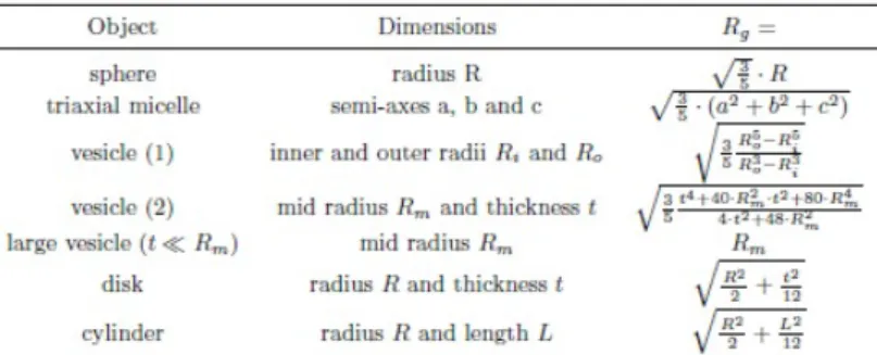
(46) P (q) = [. 3(sin QR − QR cos QR) 2 ] (QR)3. (3.8). The inter-particle structure factor S(q) depends on the type of interactions in the systems (attractive, repulsive or excluded volume). For spherical particles with low attractive interactions, a reasonable first approximation is hard-sphere potential Shs (q), given by:. Shs (q) =. 1 1 − np f (Rhs φhs ). (3.9). where Rhs is the hard sphere radius and φhs is the hard sphere volume fraction. Taking all of this into consideration the intensity of scattering equation can be rewritten as. I(q) = φV (∆ρ)2 Vp [P (q, Ri )X(Ri )]S(q, Rhs , φhs ). (3.10). As shown in figure 3.10 Shs (q) is important at low q values where it reduces the scattering intensity and produces a peak in I(q) profile at qmax = 2π/D, with D being nearest neighbor distance in the sample. For dilute, non-interacting, systems φhs ; 0 so the structure factor disappears, i.e. S(q) : 1. For interacting systems, an effective way of reducing S(q) is by diluting the system. Small Angle Neutron Scattering measurements were done on V4 at Helmholtz Zentrum Berlin (HZB), Berlin, Germany. Three configurations were used, with sampleto-detector distances of 1.6 m (λ = 4.55 Å, f whm 10%), and 15.76 m (λ = 10.2 Å, f whm10%) and respective collimation lengths of 2, 8 and 16 m, thereby covering a q range of 0.03 − 6nm−1 . The differential cross sections (absolute scaling) were obtained by the measurement of the direct beam. SANS data were fitted in absolute units using the scattering length densities and specific volumes reported in the ESI. All the measurements were carried out at 25 ◦ C and samples were loaded in 1 mm path-length circular quartz cells. 46.

(47) Figure 3.11: Picture of the SANS instrument V4 in Helmholtz Zentrum Berlin. Data reduction was done to standard procedures. The data was reduced using BerSANS, on 2D scattering patterns, to correct for the dead time, transmission, background (using cadmium at the sample position), container (substracting the empty cell, i.e. final data still contain the incoherent scattering mostly coming from the hydrogen content), detector efficiency and solid angle deviations (using the scattering by 1 mm H2 O). The SASFit program (develop at Paul Scherrer Institute, Laboratory for Neutron Scattering, Villigen, Switzerland) was used for data fitting. Model-free analysis (MFA) based on integral structural parameters (ISP). In order to check the consistency of data compared to the known compositions, and get reasonable starting parameters for further model fitting, a model free analysis is performed extracting integral structural parameters from the curves. The Porod approximation is used at high q in a range where we expect to see only the scattering from a sharp interface. The scattering can be approximated by a power law (aq −4 ) where a is the Porod coefficient if the interface is straight:. limI(q) = apq −4 + Iinc. (3.11). The Porod coefficient is used to calculate the specific area in the sample, if the molar concentration is know (C), the area per surfactant at the interface σ can be deduced: 47.

(48) 2. σ[nm ] =. [cm−1 ]10−7 C[moldm−3 ]NA 1024 P. (3.12). The Guinier approximation is used at low q (qRg− 1 ) to obtain the overall dimension of the aggregates and apart from Iinc , already determined with the Porod approximation, the require parameter are Rg the gyration radius and I0 the scattered intensity extrapolated at q = 0.. limI(q) − Iinc = I0 exp(−. (qRg )2 ) 3. (3.13). The gyration radius can be related to characteristic dimensions of simple objects (see Figure 3.12).. Figure 3.12: Relations between the gyration radius and dimensions of simple objects.. 3.2.6. High Resolution Transmission Electron Microscopy (HR-TEM). The particle size and morphology were estimated by Transmission Electron Microscopy by using Jeol 2200 FS HR-FE-TEM 200 kV. The samples were prepared by adding one droplet of final microemulsion reaction mixture to 1.5 mL of isopropanol, and dispersing by ultrasound during 1 minute. One drop of this solution was immediately deposited onto a holey-formvar carbon TEM copper grid and dried for 30 minutes. Several drops of isopropanol were deposited on the same TEM grid in order to remove excess of organic compounds. Images were analyzed using the Digital Micrograph software, version 3.4 (Gatan Inc.).. 48.

(49) Chapter 4 Results and Discussion. 49.

(50) 4.1. Microemulsion formation and characterization. 4.1.1. Microemulsion formation. The formulation of different O/W microemulsion systems was based on previous work. [24, 60] Several systems were selected for study. The first system is formed by water, surfactant (Synperonic. 91. /5 ) and oil phase. (organometallic precursor dissolved in isooctane) in different proportions.. The. compositions used were: Surfactant/Water (S/W) weight ratio varied as follows 5/95, 10/90, 15/85, 25/75, and 30/70 whilst the oil phase concentration used was 3, 5, 9, 14, and 16 wt%, one for each of the previously mentioned S/W ratios, respectively. For this system the S/O weight ratio 40/60 was approximately kept constant. This compositions are indicated in the partial phase diagram shown in Figure 4.1.. Figure 4.1: Equilibrium partial phase diagram of the selected system; with components Synperonic 91/5, isooctane and water (25◦ C.L and M indicate microemulsion and multiphasic regions, respectively.. The second system is composed by water, surfactant (Brij O10) oil phase (Pt-COD dissolved in butyl lactate) in different proportions. The Surfactant/Oil (S/O) weight ratio 50/50 was chosen and kept constant, and the water content was varied systematically (0%, 20%, 40%, 50%, 60%, 70%, 80%, 90%, 95% water content). This compositions are indicated in the phase diagram shown in Figure 4.2. 50.

(51) Figure 4.2: Microemulsion compositions selected for the system butyl-lactate/Brij O10/water.. Each sample was homogenized and the phase behavior of the samples was studied as a function of temperature and composition. The single optically isotropic, fluid and transparent phase (region of the microemulsion) was determined by visual observations for all the selected compositions. And the type of microemulsion was corroborated by conductivity measurements for some of the samples with composition (14% O/21.5% S/64.5% W).. 4.1.2. Microemulsion characterization: Conductivity. Conductivity measurements were conducted as a function of temperature. Each microemulsion was studied in the absence and presence of the organometallic precursor incorporated in the oil phase. These studies were carried out in order to characterize the type of microemulsion, by comparison of the conductivity values and the visual aspect (stability, viscosity and observation with crossed polarizers). Conductivity studies were carried out as a function of temperature for the system 25O 14 (64.5% water, 21.5% surfactant and 14% oil phase) without the metalorganic precursor and with different concentrations of the metalorganic precursor (Ce-2EH) incorporated in the oil phase. The systems under study use a non-ionic surfactant. By changing the temperature of the microemulsion, we are evaluating the hydrophilic-lipophilic properties of the 51.

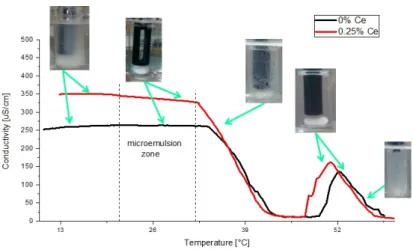
(52) surfactant in the media. This is because of the dehydration of the polar head of the surfactant as a function of the temperature. As the temperature is increased, hydrogen bonds break in the hydration layer surrounding the ethoxylated chain; this results in a smaller effective area of the headgroup and hence, increased lipophilicity. The data recorded in Figure 4.3 was accompanied by visual inspection. First, a sample without metalorganic precursor was studied, at low temperatures, the system was turbid, but it became fully transparent, fluid and isotropic between 20 and 32◦ C. This behavior indicates this is the microemulsion zone, up to this point the conductivity of the system was nearly constant and relatively high (aprox. 250 µS/cm). Above this temperature, the conductivity of the system started to decrease until reaching a minimum around 48◦ C. At this stage, the sample viscosity increased, turning slightly turbid and presenting birefringence that corresponds to a characteristic behavior of lamellar structures. Above this temperature, the conductivity started to increase again until it reached a maximum around 52◦ C aproximately 125 µS/cm (which was about 50% of the conductivity value corresponding to the microemulsion zone at 22-32◦ C). The visual aspect of the sample at this point was isotropic and slightly translucent; the conductivity values, together with the overall behavior is consistent with a transition to bicontinuous structures. Above 52◦ C the conductivity decreased once more and the sample turned milky, slightly turbid. This is an indication of the formation of an inverse microemulsion with excess water phase.. Figure 4.3: Conductivity as a function of temperature, for a sample of weight ratio 64.5/21.5/14 (W/S/O), with and without Ce precursor. 52.