Reconnection with the ideal tree : a new approach to real time search

Texto completo

(1)PONTIFICIA UNIVERSIDAD CATOLICA DE CHILE SCHOOL OF ENGINEERING. RECONNECTION WITH THE IDEAL TREE: A NEW APPROACH TO REAL-TIME SEARCH. LEÓN ILLANES FONTAINE. Thesis submitted to the Office of Research and Graduate Studies in partial fulfillment of the requirements for the degree of Master of Science in Engineering. Advisor: JORGE A. BAIER A.. Santiago de Chile, January 2014 c MMXIII, León Illanes.

(2) c MMXIII, León Illanes. Se autoriza la reproducción total o parcial, con fines académicos, por cualquier medio o procedimiento, incluyendo la cita bibliográfica que acredita al trabajo y a su autor..

(3) PONTIFICIA UNIVERSIDAD CATOLICA DE CHILE SCHOOL OF ENGINEERING. RECONNECTION WITH THE IDEAL TREE: A NEW APPROACH TO REAL-TIME SEARCH. LEÓN ILLANES FONTAINE. Members of the Committee: JORGE A. BAIER A. JUAN L. REUTTER D. CARLOS HERNÁNDEZ U. ANDRÉS GUESALAGA M. Thesis submitted to the Office of Research and Graduate Studies in partial fulfillment of the requirements for the degree of Master of Science in Engineering. Santiago de Chile, January 2014 c MMXIII, León Illanes.

(4) To my family and friends..

(5) ACKNOWLEDGEMENTS. Above all I want to acknowledge and thank my thesis advisor, Jorge Baier, and my office mate and research partner, Nicolás Rivera –whose ideas form the base over which this work is built. Without either of them, no part of the thesis would have ever existed. Alongside them, I’d like to thank Carlos Hernández, whose insight and expertise helped guide the project. I also want to thank the other members of my committee, Andrés Guesalaga and Juan Reutter, for helping expediting the final processes involved. In addition, I’d like to express my gratitude to all other sta↵ members at the Department of Computer Science, and specially acknowledge Soledad Carrión for her endless help throughout every step of my career. Of course, I wish to acknowledge my family and my friends, without whom all else is unimportant. Among them, I specifically thank the people at (and around) office O10: Andrés, Gabriel, Gonzalo, Martı́n and –once again– Nicolás. Finally, I’d like to thank my soon-to-be-wife, Andreı́ta, for always supporting me and helping me, both in relation to this work and all other activities in my life.. Real stupidity beats artificial intelligence every time. —Terry Pratchett, Hogfather (1996). v.

(6) TABLE OF CONTENTS. ACKNOWLEDGEMENTS . . . . . . . . . . . . . . . . . . . . . . . . . . . .. v. LIST OF TABLES . . . . . . . . . . . . . . . . . . . . . . . . . . . . . . . . . viii LIST OF FIGURES . . . . . . . . . . . . . . . . . . . . . . . . . . . . . . . .. ix. ABSTRACT . . . . . . . . . . . . . . . . . . . . . . . . . . . . . . . . . . . .. xi. RESUMEN . . . . . . . . . . . . . . . . . . . . . . . . . . . . . . . . . . . . .. xii. 1. INTRODUCTION . . . . . . . . . . . . . . . . . . . . . . . . . . . . . . .. 1. 1.1. Background . . . . . . . . . . . . . . . . . . . . . . . . . . . . . . . .. 1. 1.1.1. State-Space Problems . . . . . . . . . . . . . . . . . . . . . . . . .. 3. 1.1.2. Heuristic Search . . . . . . . . . . . . . . . . . . . . . . . . . . . .. 4. 1.1.3. Incremental Heuristic Search . . . . . . . . . . . . . . . . . . . . .. 7. 1.1.4. Real-Time Heuristic Search . . . . . . . . . . . . . . . . . . . . .. 9. 1.2. Thesis Work . . . . . . . . . . . . . . . . . . . . . . . . . . . . . . . .. 13. 1.2.1. Major Contributions . . . . . . . . . . . . . . . . . . . . . . . . .. 13. 1.2.2. Future Work . . . . . . . . . . . . . . . . . . . . . . . . . . . . . .. 14. 2. ARTICLE SUBMITTED TO JOURNAL OF ARTIFICIAL INTELLIGENCE RESEARCH . . . . . . . . . . . . . . . . . . . . . . . . . . . . . . . . . . .. 15. 2.1. Introduction . . . . . . . . . . . . . . . . . . . . . . . . . . . . . . . .. 15. 2.2. Background . . . . . . . . . . . . . . . . . . . . . . . . . . . . . . . .. 18. 2.2.1. Real-Time Search . . . . . . . . . . . . . . . . . . . . . . . . . . .. 19. 2.3. Searching via Tree Reconnection . . . . . . . . . . . . . . . . . . . . .. 22. 2.3.1. The Ideal Tree . . . . . . . . . . . . . . . . . . . . . . . . . . . . .. 22. 2.3.2. Following and Reconnecting . . . . . . . . . . . . . . . . . . . . .. 24. 2.4. Satisfying the Real-Time Property . . . . . . . . . . . . . . . . . . . .. 27. 2.4.1. FRIT with Real-Time Heuristic Search Algorithms . . . . . . . .. 29 vi.

(7) 2.4.2. FRIT with Bounded Complete Search Algorithms . . . . . . . . .. 33. 2.5. Theoretical Analysis . . . . . . . . . . . . . . . . . . . . . . . . . . . .. 34. 2.5.1. Proofs for InTree[c] . . . . . . . . . . . . . . . . . . . . . . . . .. 35. 2.5.2. Termination and bound for FRITRT . . . . . . . . . . . . . . . . .. 36. 2.5.3. Termination and bound for FRIT . . . . . . . . . . . . . . . . . .. 37. 2.5.4. Convergence . . . . . . . . . . . . . . . . . . . . . . . . . . . . . .. 38. 2.6. Empirical Evaluation . . . . . . . . . . . . . . . . . . . . . . . . . . .. 39. 2.6.1. Analysis of the results for real-time search algorithms . . . . . . .. 41. 2.6.2. Analysis of the results for incremental algorithms modified to satisfy the real-time property . . . . . . . . . . . . . . . . . . . . . .. 42. 2.6.3. Comparison of the two approaches . . . . . . . . . . . . . . . . . .. 45. 2.7. Related Work . . . . . . . . . . . . . . . . . . . . . . . . . . . . . . .. 45. 2.7.1. Incremental and Real-Time Heuristic Search Algorithms . . . . .. 45. 2.7.2. Bug Algorithms . . . . . . . . . . . . . . . . . . . . . . . . . . . .. 47. 2.8. Summary . . . . . . . . . . . . . . . . . . . . . . . . . . . . . . . . . .. 49. References . . . . . . . . . . . . . . . . . . . . . . . . . . . . . . . . . . . . . .. 51. vii.

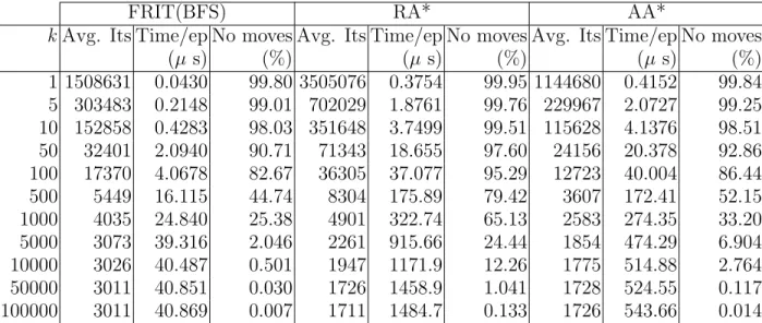
(8) LIST OF TABLES. 2.1. Relationship between search expansions and number of iterations in which the agent does not move in games maps. The table shows a parameter k for each algorithm. In the case of AA* and Repeated A* the parameter corresponds to the number of expanded states. In case of FRIT, the parameter corresponds to the number of visited states during an iteration. In addition, it shows average time per search episode (Time/ep), and the percentage of iterations in which the agent was not moved by the algorithm with respect to the total number of iterations (No moves). . . . . . . . .. 44. viii.

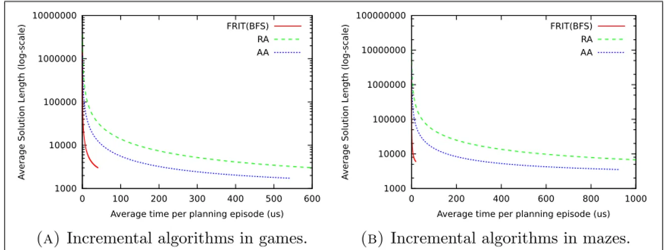
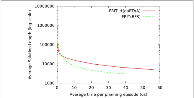
(9) LIST OF FIGURES. 1.1. A heuristic depression in a graph. The numbers represent the heuristic values for each state. . . . . . . . . . . . . . . . . . . . . . . . . . . . . .. 1.2. 12. A heuristic depression in a grid pathfinding problem. The numbers represent the heuristic value for each cell of the grid. Black cells are obstacles. The gray colored cells are a heuristic depression. . . . . . . . .. 2.1. 12. An illustration of some of the steps of an execution over a 4-connected grid pathfinding task, where the initial state is cell D3, and the goal is E6. The search algorithm A is breadth-first search, which, when expanding a cell, generates the successors in clockwise order starting with the node to the right. The position of the agent is shown with a black dot. (a) shows the true environment, which is not known a priori by the agent. (b) shows the p pointers which define the ideal tree built initially from the Manhattan heuristic. Following the p pointers, the algorithm leads the agent to D4, where a new obstacle is observed. D5 is disconnected from T and GM , and a reconnection search is initiated. (c) shows the status of T after reconnection search expands state D4, finding E4 is in T . The agent is then moved to E4, from where a new reconnection search expands the gray cells shown in (d). The problem is now solved by simply following the p pointers. . . . . . . . . . . . . . . . . . . . . . . . . . . . . . . . . . . . .. 28. 2.2. Real-time algorithms: Total Iterations versus Time per Episode . . . . .. 42. 2.3. Incremental algorithms: Total Iterations versus Time per Episode . . . .. 43. 2.4. Incremental algorithms: Total Iterations versus Time per Episode (zoomed) 43. 2.5. Comparison of FRIT using a real-time algorithm versus FRIT as an incremental algorithm in games benchmarks. . . . . . . . . . . . . . . . .. 46 ix.

(10) 2.6. Bug2 (a) and FRIT (b) in a pathfinding scenario in which the goal cell is E10 and the initial cell is E2. The segmented line shows the path followed by the agent. . . . . . . . . . . . . . . . . . . . . . . . . . . . . . . . . .. 49. x.

(11) ABSTRACT. In this thesis we present FRIT, a simple approach for solving single-agent deterministic search problems under tight time constraints in partially known environments. Unlike traditional Real-Time Heuristic Search (RTHS) algorithms, FRIT does not search for the goal but rather searches for a path that connects the current state with a so-called ideal tree T . Such a tree is rooted in the goal state and is built initially using a user-given heuristic h. When the agent observes that an arc in the tree cannot be traversed in the actual environment, it removes such an arc from T and then carries out a reconnection search whose objective is to find a path between the current state and any node in T . Reconnection is done using an algorithm that is passed as a parameter to FRIT. As such, FRIT is a general framework that can be applied to many search algorithms. If such a parameter is an RTHS algorithm, then the resulting algorithm can be an RTHS algorithm. We show, however, that FRIT may be fed with a complete blindsearch algorithm, which in some applications with tight time constraints (including video games) may be acceptable and, perhaps, preferred to a pure RTHS algorithm. We evaluate over standard grid pathfinding benchmarks including game maps and mazes. Results show that FRIT, used with RTAA*, a standard RTHS algorithm, outperforms RTAA* significantly; by one order of magnitude under tight time constraints. In addition, FRIT(daRTAA*) substantially outperforms daRTAA*, a state-of-the-art RTHS algorithm, usually obtaining solutions 50% cheaper on average when performing the same search e↵ort. Finally, FRIT(BFS), i.e., FRIT using breadth-first-search, obtains very good quality solutions and is perhaps the algorithm that should be preferred in video game applications.. Keywords: Heuristic Search, Real-Time Heuristic Search, Incremental Search, Heuristic Learning, A*, Learning Real-Time A*, FRIT xi.

(12) RESUMEN. En esta tesis se presenta FRIT, un algoritmo simple que resuelve problemas de búsqueda determinı́stica para un agente, en ambientes parcialmente conocidos bajo restricciones de tiempo estrictas. A diferencia de otros algoritmos de búsqueda heurı́stica en tiempo real (BHTR), FRIT no busca el objetivo: busca un camino que conecte el estado actual con un árbol ideal T . El árbol tiene su raı́z en el objetivo y se construye usando la heurı́stica h. Si el agente observa que un arco en el árbol no existe en el ambiente real, lo saca de T y realiza una búsqueda de reconexión para encontrar un camino que lleve a cualquier estado en T . La búsqueda de reconexión se lleva a cabo por medio de otro algoritmo. Ası́, FRIT puede aplicarse sobre muchos algoritmos de búsqueda y si se trata de un algoritmo para BHTR, el algoritmo resultante puede serlo también. Por otro lado, mostramos que FRIT también puede usar un algoritmo de búsqueda ciega, resultando en un algoritmo que puede ser aceptable para aplicaciones con restricciones de tiempo estrictas (como videojuegos) y que incluso puede ser preferible a un algoritmo de BHTR. Evaluamos el algoritmo en problemas estándares de búsqueda en grillas, incluyendo mapas de videojuegos y laberintos. Los resultados muestran que FRIT usado con RTAA*—un algoritmo de BHTR tı́pico—es significativamente mejor que RTAA*, con mejoras de hasta un orden de magnitud bajo restricciones de tiempo estrictas. Además, FRIT(daRTAA*) supera a daRTAA*—el estado del arte en BHTR—y en promedio obtiene soluciones un 50% menos costosas usando el mismo tiempo total. Finalmente, FRIT usando búsqueda en amplitud obtiene soluciones de muy buena calidad y puede ser ideal para aplicaciones de videojuegos.. Palabras Claves: Búsqueda Heurı́stica, Búsqueda en Tiempo Real, Búsqueda Incremental, Aprendizaje de Heurı́sticas, A*, FRIT xii.

(13) 1. INTRODUCTION. 1.1. Background Many algorithmic problems in Computer Science are formulated as search tasks, in which the goal is to find a solution for the original problem. Indeed, search algorithms are one of the core tools used in the development of Artificial Intelligence, where so called rational agents act based on their observation of the environment and attempt to achieve positive outcomes (Russell & Norvig, 2010, Ch. 1). Many of the problems solved by such agents are naturally modeled as search problems. Some examples are pathfinding for field robotics and general planning of action sequences. Generally, many other problems can be formalized as state-space problems. This formulation defines a space of states and operations that describe the environment, where the operations modify the environment and change the state. In this setting, we aim to find a set of operations that can modify an initial state into a goal state. This can be modeled as a graph, where states are nodes and operations are the edges that connect di↵erent nodes. Here, a solution is a sequence of operations forming a path from the initial state to the goal state. This path can be optimized for di↵erent criteria, such as length or cost. As an example, we can see how this approach can be used to model puzzle problems such as the Rubik’s Cube. A 3 ⇥ 3 ⇥ 3 cube is formed by 26 visible smaller cubes, called cubies. Of these, 6 represent the centers of each face and cannot be moved. The remaining 20 cubies can be either one of the 8 corners or one of the 12 edges. Each of the corner cubies has 3 colors, whereas the edges have 2. This uniquely identifies each cubie, and can be therefore used to identify the state of the full cube as a list describing the position of each of the 20 movable cubies with respect to the static frame of reference defined by the 6 unmovable ones. There is a set of 12 (or 18) primitive or fundamental operations that can be performed on every state. These correspond to rotating any of the 6 faces 90 in 1.

(14) either direction (traditionally, rotating 180 is considered a separate action, although it could be represented as two 90 rotations in the same direction). This way, a graph representation for this problem has a node for each state, and each node is connected to 12 (or 18) other nodes through the corresponding operators. Note that even considering some other restrictions regarding the respective positions of the fixed center cubies, such a representation has over 4.3 ⇥ 1019 states (Korf, 1997). However, it has been computationally proved that for every state in the graph resulting from considering 18 operators, there exists at least one path to the goal of length shorter or equal to 20 (Rokicki, Kociemba, Davidson, & Dethridge, 2013). The general problem of finding optimal paths in graphs has been studied extensively both in Mathematics and Computer Science, and many algorithms have been designed specifically for this. Algorithms employing uninformed search strategies make no assumptions on the structure and characteristics of the problem, and work well in the general case. However, they can be inefficient when dealing with very large state spaces, such as the ones found in many real-world applications. Informed search strategies aim to solve this issue by means of heuristic functions that try to guide the search e↵orts towards the goal, avoiding unnecessary computation. The heuristics are designed specifically for each application, and often attempt to imitate techniques used by humans when dealing with similar tasks. The area of Artificial Intelligence concerned with heuristics and informed search is Heuristic Search. For some applications, additional constraints and limitations are placed upon the formalization of the problem. For instance, the information available for a robot moving in an unknown environment can be limited to what the robot has already observed, or the amount of computation allowable before moving a character in a real-time video game is limited. This thesis is concerned with problems that combine both of this constraints, in what we call Real-Time Heuristic Search in unknown environments.. 2.

(15) 1.1.1. State-Space Problems As discussed above, many problems in Artificial Intelligence and Computer Science can be formulated as state-space search problems, and can subsequently be solved with search techniques. Below, we formalize state-space search problems. A state-space search problem is defined as a tuple P = (S, A, c, sstart , G). The directed graph (S, A) represents the state-space, where S is the set of all possible states and A is the set of operations or actions that can transition the problem through di↵erent states. This way, if a = (s, t) and a 2 A, then it is possible to transition from state s to state t by executing action a. sstart 2 S corresponds to the initial state and G ✓ S is the set of all goal states. The function c : A ! R+ 0 assigns costs to the actions, so that an agent performing action a will incur in a cost of c(a). Note that without loss of generality, we can assume one single goal state g, such that G = {g}. To use this formulation with a problem that does have multiple goal states we can add a new state, g, and connect every state s 2 G to g with an action a = (s, g) such that c(a) = 0. Below, we mostly use this formulation. A sequence of states. = s0 , s1 , . . . , sn such that for every i < n, we have. (si , si+1 ) 2 A is called a path. Any path starting in sstart and finishing in g is a solution for P . An optimal solution is one that minimizes the sum of the costs of the actions used. Depending on the application, the goal can be to find an optimal path or to quickly find a suboptimal path. The standard algorithm for finding an optimal path is Dijkstra’s Algorithm. Pseudo-code for the algorithm is shown in Algorithm 1. In very general terms, this algorithm extends the search outwards from sstart until it reaches g. More specifically, it searches the states of the problem in order of cumulative distance from sstart , ensuring each node is reached through an optimal path. Using an appropriate data structure for the priority queue Q, the algorithm can run in O(|A| + |S| log |S|) steps (Fredman & Tarjan, 1984).. 3.

(16) Algorithm 1: Dijkstra’s Algorithm Input: S, A, c, sstart , G Output: A sequence of states representing the shortest path from sstart to a state in G. 1 Initialization: 2 for each x 2 S do 3 x.distance 1 4 x.expanded F alse 5 x.previous null 6 7 8 9 10 11 12. 13 14 15 16 17 18 19 20. sstart .distance 0 Insert sstart into priority queue Q. Search: while Q is not empty do Remove s from Q with smallest distance. if s 2 G then return // The solution can be extracted from the previous pointers. s.expanded T rue for each n 2 S such that (s, n) 2 A do d s.distance + c(s, n) if d < n.distance then n.distance d n.previous s if ¬n.expanded then Insert n into Q.. 1.1.2. Heuristic Search For some real-world applications where the number of states is large, Dijkstra’s Algorithm is somewhat inefficient. To solve these issue, we can guide the search by using information specific to the problems involved. Usually, we include this information into the search as a heuristic function, a function that somehow ranks the various available states. In our formal setting, a heuristic is defined as a function h : S ! R+ 0 , that assigns to each state s 2 S an estimated value of the cost needed to go from s to g through a path in the state-space graph. We define the perfect or optimal heuristic 4.

(17) h⇤ as the heuristic that correctly estimates the minimum distances for each state. This way, for any s 2 S, h⇤ (s) corresponds to the cost of the best path between s and g. Additionally, we say that a heuristic h is admissible if for every state s 2 S. it holds that h(s)  h⇤ (s). That is, a heuristic is admissible if it never overestimates the distances. Finally, we say that h is consistent if for every (s, t) 2 A it holds that h(s)  c(s, t) + h(t), and for every g 2 G it holds that h(g) = 0. It is easy to prove that all consistent heuristics are also admissible.. 1.1.2.1. The A* Algorithm The standard algorithm used for finding shortest paths in Heuristic Search is called A* (Hart, Nilsson, & Raphael, 1968). It works by maintaining and updating a merit function f that estimates, for each state s, the cost of an optimal path going from sstart to g and passing through s. For a given state s 2 S, it is defined as f (s) = g(s) + h(s), where g(s) corresponds to the accumulated cost of the best path already discovered that goes from sstart to s. Initially, g(sstart ) = 0 and g(s) = 1 for all other states. Pseudo-code for this algorithm is shown in Algorithm 2. A* uses two lists, Open and Closed, which intuitively represent the information known for each state. As states are discovered, they are put in the Open list. When the state is expanded (i.e.: all its neighbors are discovered) it is moved to the Closed list. Whenever a shorter path to a state in Closed is discovered, the state is moved back to Open, to eventually check if this implies better paths for any of it neighbors. Note that the order in which the states are explored and expanded depends on the merit function f , which is determined by both the heuristic function h and the costs of the discovered paths. This contrasts with Dijkstra’s Algorithm, where the order of expansion is determined exclusively by the costs. Indeed, if h(s) = 0 for all states s 2 S, and assuming tie-breaking for states with the same merit is done in the same 5.

(18) Algorithm 2: The A* Algorithm Input: S, A, c, sstart , G, h(·) Output: A sequence of states representing the shortest path from sstart to a state in G. 1 Initialization: 2 Closed ? 3 Open {sstart } 4 for each s 2 S do 5 g(s) 1 6 s.previous = null 7 8 9 10 11 12 13 14. 15 16 17 18 19 20 21 22 23. g(sstart ) 0 f (sstart ) h(sstart ) Search: while Open is not empty do Remove s from Open with minimum f (s). Insert s into Closed. if s 2 G then return // The solution can be extracted from the previous pointers. for each n 2 S such that (s, n) 2 A do if g(s) + c(s, n) < g(n) then n.previous s g(n) g(s) + c(s, n) f (n) g(n) + h(n) if n 2 Closed then Remove n from Closed. if n 62 Open and n 62 Closed then Insert n into Open.. way, then A* expands the states in the same order as Dijkstra’s Algorithm and gives identical results. Other relevant properties of A* are that if h is admissible, it will return an optimal solution (Hart et al., 1968). Moreover, if h is consistent then A* is optimally efficient and no algorithm can be shown to expand fewer states than A* when using the same heuristic (Edelkamp & Schrödl, 2011) and tie-breaking strategy. Furthermore, given two di↵erent consistent heuristics h1 and h2 such that h2 (s). h1 (s) for 6.

(19) all states s 2 S, A* using h2 will expand fewer states than A* using h1 . Intuitively, this means that the performance of A* improves when the heuristic is a better approximation. This motivates the concept of heuristic learning, which has been a key tool for real-time heuristic search and is further discussed in the following sections. Additionally, A* can be easily used to find suboptimal paths by using weights that modify an admissible heuristic, making it inadmissible. Typically, this is done by redefining the merit function f to f (s) = g(s) + w · h(s). This is known as the Weighted A* Algorithm (wA*), and—when compared to simply using A* with the admissible heuristic—will usually result in a much faster performance time wise, albeit at a loss in solution quality (i.e.: cost). When using an admissible heuristic and a weight w, the obtained solution is suboptimal by at most a factor of w. 1.1.3. Incremental Heuristic Search An alternative method for speeding up searches is to use Incremental Search. This technique is used when searches are done repeatedly in the same or similar environment, so algorithms attempt to reuse information obtained in previous e↵orts in order to solve newer problems faster than by doing a completely new search. It is particularly relevant when dealing with dynamic environments—such as those encountered by most applications involving the real, physical world or by applications involving multiple independent agents. Here, planning needs to be repeated as the state-space graph changes. Many uninformed algorithms focused on finding optimal paths on these graphs have been proposed in literature. Indeed, Deo and Pang (1984) refer to several such algorithms published in the 1960s. Since then, algorithms that combine Incremental Search with Heuristic Search have been developed. Some examples are D* (Stentz, 1995), D*Lite (Koenig & Likhachev, 2002), Lifelong Planning A* (Koenig & Likhachev, 2001; Koenig, Likhachev, & Furcy, 2004) and Adaptive A* (Koenig & Likhachev, 2006a). These algorithms can be used to solve search problems in initially unknown environments, which are frequently seen in the field of Robotics. A robot moving in an unknown terrain which 7.

(20) knows its relative position with regards to a goal can plan a path to it by assuming all unknown areas to be traversable. This is known as planning with the free-space assumption. When traveling through the resulting path, the robot might encounter obstacles and will need to replan. 1.1.3.1. Adaptive A* As mentioned above, Adaptive A* (AA*) is an incremental search algorithm that guides the search with the use of a heuristic function. It is based on A*, and as such has certain guarantees on optimality. E↵ectively, if the given heuristic is consistent, then at every point of the search the planned path-to-go is optimal with regards to the currently known information. Algorithm 3 shows pseudo-code for an implementation of AA* designed for use in pathfinding in initially partially known terrain. Algorithm 3: Adaptive A* Input: S, A, c, sstart , G, h(·) E↵ect: The agent is moved from sstart to a state in G, if such a path exists. 1 Initialization: 2 Observe the environment around sstart and remove non-traversable arcs from A. 3 s sstart 4 Search: 5 while s 62 G do 6 Call A*(S, A, c, s, G, h(·)). Extract a solution path and keep the Open and Closed lists. 7 f⇤ minx2Open f (x) 8 for each x 2 Closed do 9 h(x) f ⇤ g(x) 10. Move the agent through the path . While moving, observe the environment and remove non-traversable arcs from A. Stop if an arc in is removed from A.. The algorithm works by repeatedly searching with A*, and uses the returned path and the Open and Closed lists (Line 6). The agent is moved through the path and the state-space graph is updated according to observation of the agent’s 8.

(21) environment (Line 10). Whenever an arc in the path is removed, the movement stops and the path is replanned. Finally, note that Lines 7–9 modify the heuristic function. This is known as heuristic learning and is used here to ensure that information discovered in a planning episode of the algorithm can be used in further planning stages. Heuristic learning is a key idea in real-time heuristic search, and will be discussed in more detail below.. 1.1.4. Real-Time Heuristic Search Certain search applications impose restrictions on the amount of time that can pass between the execution of two consecutive actions. E↵ectively, this limits the amount of computation that can be performed by an agent before deciding on a path to follow. One of the original goals for the field was to limit the search to only consider states in a vicinity of the agent (Korf, 1990). This idea is sometimes called agentcentered search (Koenig, 2001). The underlying motivation for this is that it represents an efficient way of handling problems in very large space-states. For this thesis, we are mostly concerned with the application of real-time heuristic search algorithms in a priori unknown environments. One of the most straightforward applications of this is pathfinding in video games, where characters must often move automatically in a partially known map. For interactivity reasons, systems are sometimes given only a few milliseconds to decide where to move a number of di↵erent characters (Bulitko, Björnsson, Sturtevant, & Lawrence, 2011). A di↵erent application considers very fast robots, which physically move in real-time. 1.1.4.1. Learning Real-Time A* Most real-time heuristic search algorithms are variants of one of the original algorithms proposed by Korf (1990), Learning Real-Time A* (LRTA*). As such, most of these algorithms share a familiar structure based around four distinct parts: observing, planning, learning, and moving. 9.

(22) As for Adaptive A*, the learning process corresponds to heuristic learning. In general terms, the goal of learning is to update the heuristic to consider some of the information discovered during search. In Algorithm 4 we show the pseudo-code for an implementation of LRTA*. Algorithm 4: Learning Real-Time A* Input: S, A, c, sstart , G, h(·) E↵ect: The agent is moved from sstart to a state in G, if such a path exists. 1 Initialization: 2 s sstart 3 Search: 4 while s 62 G do 5 Observe the environment around the location of the agent and remove from A all newly discovered non-traversable edges. 6 n arg mint:(s,t)2A c(s, t) + h(t) 7 if h(s) < c(s, n) + h(n) then 8 h(s) c(s, n) + h(n) 9. Move the agent to n, setting s. n.. Note that the four concepts defined are clearly represented in the algorithm. Indeed, in Line 5 the agent observes the environment, updating the relevant information. Then, in Line 6, the agent plans which of its direct neighbors it will move to. Lines 7 and 8 define how the heuristic is updated, which corresponds to the learning stage. Finally, Line 9 moves the agent according to the plan. The learning process is focused on inflating the heuristic values of visited states as much as possible without making the heuristic inconsistent. Therefore, the update sets the heuristic of a state s to the highest possible value that does not break consistency, which is mint:(s,t)2A c(s, t) + h(t). Variants of LRTA* algorithm modify the di↵erent stages, usually performing more elaborate computations in some of them. For example, both RTAA* (Koenig & Likhachev, 2006b) and LSS-LRTA* (Koenig & Sun, 2009) modify the planning and learning stages, allowing for a longer path planned and more heuristic values updated in each iteration. Both of these algorithms use—as their planning stage—an 10.

(23) A* search that stops whenever a predetermined number of states has been expanded. They di↵er in how they perform the heuristic update. LSS-LRTA* extends the idea used in LRTA*, inflating the heuristic as much as possible in a larger region. RTAA* uses the same the update strategy as AA*, which results in a faster procedure where the states’ heuristic values are not raised as much. 1.1.4.2. Convergence One of the key properties of LRTA* is that repeatedly running the algorithm over the same problem will continue to increase the heuristic values of the visited nodes until they converge to optimal values. That is, running sufficient trials over the same problem without reseting the heuristic function will inflate it for states in the visited paths until it reaches h⇤ . Eventually, all states in the optimal path between sstart and G will have accurate heuristic values and running the algorithm again will result in the optimal solution. Many real-time search algorithms share this property, which we call optimal convergence. Additionally, some algorithms converge to suboptimal solutions. The number of repeated trials needed for convergence varies between algorithms, problem domains and problem instances. 1.1.4.3. Heuristic Depressions Among the most important issues involved is real-time search, is the fact that heuristics often contain depressions. Intuitively, depressions are bounded regions of the state-space that do not contain a goal state and where the heuristic values are comparatively low with respect to the heuristic values of states just outside the region. It is well known that real-time search algorithms can perform poorly in these regions. Indeed, Korf (1990) provides the example shown in Figure 1.1. Here, if an agent based on LRTA* starts in one of the two nodes of the graph that have heuristic value 1, it will move back and forth between them increasing their heuristic values in small steps until at least one of them reaches a heuristic value of 5. 11.

(24) 5. 1. 5. 1. Figure 1.1. A heuristic depression in a graph. The numbers represent the heuristic values for each state.. Figure 1.2 shows an example of how a heuristic depression can naturally occur in simple pathfinding problems in grids using a common heuristic function. This heuristic is known as the Manhattan Heuristic, and it estimates the cost to the goal (marked as G) as the sum of the horizontal and vertical distances.. 10. 9. 8. 7. 6. 5. 4. 3. 9. 8. 7. 8. 7. 6. 5. 4. 3. 1. 7. 6. 5. 4. 3. 2. G. 8. 7. 6. 5. 4. 3. 1. 9. 8. 7. 10. 9. 8. 2. 2 7. 6. 5. 4. 3. Figure 1.2. A heuristic depression in a grid pathfinding problem. The numbers represent the heuristic value for each cell of the grid. Black cells are obstacles. The gray colored cells are a heuristic depression.. Algorithms such as LSS-LRTA* are not very e↵ective when dealing with heuristic depressions. Although learning the heuristic correctly in a big enough are will ensure that the depressions are mostly avoided, this approach will not work when the relevant regions are larger that what is feasible to learn in limited time. More elaborate 12.

(25) approaches consider removing or pruning states that are proved to be not conducive towards the goal (Sharon, Sturtevant, & Felner, 2013). A di↵erent family of algorithms attempts to actively identify depressions and escape them quickly (Hernández & Baier, 2012).. 1.2. Thesis Work The goal of the research project described here is to apply a new approach to real-time search. Although the approach shares similarities with both Incremental Search and traditional Real-Time Heuristic Search, we believe the core idea behind it has not been previously considered in literature. To understand the motivation behind this idea, we can somewhat reformulate search problems in initially unknown environments. As we have discussed in the previous sections, the planning stage of algorithms for these problems is repeated when previous plans are discovered to be incorrect. Usually, each planning stage is treated as a new search problem in which the objective is to find a path to a goal state. We propose that the objective could rather be to find a path to an area where we believe finding a path to the goal will be easy. Basically, the agent should move to regions in which the heuristic seems to be correct. This is similar to what is described by Hernández and Baier (2012), but our approach is very di↵erent in spirit. 1.2.1. Major Contributions The major contributions presented in this thesis are outlined below. • We describe FRIT, a new family of search algorithms for initially partially known environments. • We show two di↵erent ways to use FRIT with real-time constraints. • We prove that both versions of our algorithm terminate, and we give explicit bounds on the returned solutions. 13.

(26) • We prove that both algorithms converge after a second trial run. • We empirically show that our algorithms perform well. Tests were run on standard grid pathfinding benchmarks (Sturtevant, 2012), where FRIT significantly outperforms state-of-the-art RTHS algorithms. 1.2.2. Future Work Future work in this area can be based upon applying the proposed algorithms to other problems where real-time heuristic search is relevant. Some of these problems void some of the key assumptions made by algorithms such as LRTA*. For example, the number of states in the vicinity of an agent is usually assumed to be constantly bounded, which is not true in a dense graph. We believe our algorithms may be well suited for some of these situations.. 14.

(27) 2. ARTICLE SUBMITTED TO JOURNAL OF ARTIFICIAL INTELLIGENCE RESEARCH 2.1. Introduction Real-Time Heuristic Search (Korf, 1990) is an approach to solving single-agent search problems when a limit is imposed on the amount of computation that can be used for deliberation. It is used for solving problems in which agents have to start moving before a complete search algorithm can solve the problem and is especially suitable for problems in which the environment is only partially known in advance. An application of real-time heuristic search algorithms is goal-directed navigation in video games (Bulitko et al., 2011) in which computer characters are expected to find their way in partially known terrain. Game-developing companies impose a constant time limit on the amount of computation per move close to one millisecond for all simultaneously moving characters (Bulitko et al., 2011). As such, real-time search algorithms are applicable since they provide the main loop with quick moves that allow implementing continuous character moves. Standard Real-Time Heuristic Search algorithms—e.g., LRTA*(Korf, 1990) or LSS-LRTA* (Koenig & Sun, 2009)—however, are not algorithms of choice for videogame developers, since they will require to re-visit many states in order to escape socalled heuristic depressions, producing back-and-forth movements, also referred to as scrubbing (Bulitko et al., 2011). The underlying reason for this behavior is that the heuristic used to guide search must be updated—in a process usually referred to as heuristic learning—whenever new obstacles are found. To exit so-called heuristic depressions, the agent may need to revisit a group of states many times (Ishida, 1992). By exploiting preprocessing (e.g. Bulitko, Björnsson, Lustrek, Schae↵er, & Sigmundarson, 2007; Bulitko, Björnsson, & Lawrence, 2010; Hernández & Baier, 2011), one can produce algorithms based on Real-Time Heuristic Search algorithms that 15.

(28) will control the agent in a way that is sensible to the human observer. Give a map of the terrain, these algorithms generate information o✏ine that can later be utilized online by a Real-Time Search algorithm to find paths very quickly. Unfortunately, preprocessing is not applicable in all settings. For example if one wants to implement an agent which has no knowledge of the terrain, there is no map that is available prior to search and hence no preprocessing can be carried out. On the other hand, when knowledge about the terrain is only partial (i.e., the agent may know the location of some of the obstacles but not all of them), using a plain Real-Time Heuristic Search along with partial information about the map obtained from preprocessing (i.e., a perfect heuristic computed for the partially known map) may still result in the same performance issues described above. In this paper we present FRIT, a real-time search algorithm that does not necessarily rely on heuristic learning to control the agent, and that produces high-quality solutions in partially known environments. While easily motivated by game applications, our algorithm is designed for general search problems. An agent controlled by our algorithm always follows the branch of a tree containing a family of solutions. We call such a tree the ideal tree because the paths it contains are solutions in the world that is currently known to the agent, but such solutions may not be legal in the actual world. As the agent moves through the states in the ideal tree it will usually encounter states that are not accessible and which block a solution in the ideal tree. When this happens, a secondary algorithm is used to perform a search and reconnect the current state with another state known to be in the ideal tree. After reconnection succeeds the agent is again on a state of the ideal tree, and it can continue following a branch. We evaluated our algorithm over standard game and maze pathfinding benchmarks using both a blind, breadth-first search algorithm and two di↵erent real-time search algorithms for reconnection. Even though our algorithm does not guarantee optimality, solutions returned, in terms of quality and total time, are significantly. 16.

(29) better than those returned by the state-of-the-art real-time heuristic search algorithms we compared to, when the search e↵ort is fixed. Upon inspection of the route followed by the agent, we observe that when using blind-search algorithms for reconnection they do not contain back-and-forth, “irrational” movements, and that indeed they look similar to solutions returned by so-called bug algorithms (LaValle, 2006; Taylor & LaValle, 2009) developed by the robotics community. As such, it usually detects states that do not need to be visited again—sometimes referred to as deadends or redundant states (Sturtevant & Bulitko, 2011; Sharon et al., 2013)—without implementing a specific mechanism to detect them. We also compared our algorithm to incremental heuristic search algorithms that can be modified to behave like a real-time search algorithm. We find that, although FRIT does not reach the same solution quality, it can obtain solutions that are significantly better when the time deadline is tight (under 40µ sec). Our algorithm is extremely easy to implement and, in case there is sufficient time for pre-processing, can utilize techniques already described in the literature, like so-called compressed path databases (Botea, 2011), to compute an initial ideal tree. Furthermore, we provide proofs for termination of the algorithm using realtime search and blind-search for reconnection, and provide a bound on the number of moves required to find a solution in arbitrary graphs. Some of the contributions presented in this paper have been published in conference papers (Rivera, Illanes, Baier, & Hernandez, 2013). This articles extends the work and includes new material that has not been presented before. In particular: • We describe a method to use our algorithm with a real-time search algorithm passed as a parameter, and evaluate the results obtained when using two di↵erent real-time algorithms. • We provide proofs for the termination of algorithms obtained by using the aforementioned method, and a general proof for convergence applicable to all the algorithms we propose. 17.

(30) • We incorporate a small optimization that a↵ects the InTree[c] function described in Section 2.3. • We extend some of the previous empirical results by including maze benchmarks, which had not been previously considered, and by evaluating on more problem instances. The rest of the paper is organized as follows. In Section 2.2 we describe the background necessary for the rest of the paper. In Section 2.3 we describe a simple version of our algorithm that is not real-time. In Section 2.4 we describe two alternative ways to make the algorithm satisfy the real-time property. In Section 2.5 we present a theoretical analysis, followed by a description of our experimental evaluation in Section 2.6. We then describe other related work, and finish with a summary.. 2.2. Background The search problems we deal with in this paper can be described by a tuple P = (G, c, sstart , g), where G = (S, A) is a digraph that represents the search space. The set S represents the states and the arcs in A represent all available actions. State sstart 2 S is the initial state and state g 2 S is the goal state. We assume that S is finite, that A does not contain elements of form (s, s), that G is such that g is reachable from all states reachable from sstart . In addition, we have a non-negative cost function c : A ! R which associates a cost with each of the available actions. Naturally, the cost of a path in the graph is the sum of the costs of the arcs in the path. Finally g 2 S is the goal state. Note that even though our definition considers a single goal state it can still model problems with multiple goal states since we can always transform a multiple-goal problem into a single-goal problem by adding a new state g to the graph and connecting the goals in the original problem to g with a zero-cost action. We define the distance function dG : S ⇥ S ! R such that dG (s, t) denotes the cost of a shortest path between s and t in the graph G. A heuristic for a 18.

(31) search graph G is a non-negative function h : S ! R such that h(s) estimates dG (s, g). We say that h is admissible if h(s)  dG (s, g), for all s 2 S. In addition, we say a heuristic h is consistent if for every pair (s, t) 2 A it holds that h(s)  c(s, t) + h(t), and furthermore that h(g) = 0. It is simple to prove that consistency implies admissibility. 2.2.1. Real-Time Search Given a search problem P = (G, c, sstart , g), the objective of a real-time search algorithm is to move an agent from sstart to g, through a low-cost path. The algorithm should satisfy the real-time property, which means that the agent is given a bounded amount of time for deliberating, independent of the size of the problem. After deliberation, the agent is expected to move. After such a move, more time is given for deliberation and the loop repeats. Most Real-Time Heuristic Search algorithms rely on the execution of a bounded but standard state-space search algorithm (e.g., A*, Hart et al., 1968). In order to apply such an algorithm in partially known environments, they carry out their search in a graph which may not correspond to the graph describing the actual environment. In particular, in pathfinding in grid worlds, it is assumed that the dimensions of the grid are known, and to enable search a free-space assumption (Zelinsky, 1992) is made, whereby grid cells are regarded as obstacle-free unless there is sufficient information to the opposite. Below we define a version of the free-space assumption for use with general search problems. We assume a certain search graph GM is given as input to the agent. Such a graph reflects what the agent knows about the environment, and is kept in memory throughout execution. We assume that this graph satisfies the following generalized version of the free-space assumption: if the actual search graph is G = (S, A), then GM is a spanning supergraph of G, i.e. GM = (S, A0 ), with A ✓ A0 . Note that because GM is a supergraph of G then dGM (s, t)  dG (s, t) for all s, t 2 S, and that if h is admissible for GM then so it is for G. 19.

(32) While moving through the environment, we assume the agent is capable of observing whether or not some of the arcs in its search graph GM = (S, A0 ) are present in the actual graph. Specifically, we assume that if the agent is in state s, it is able to sense whether (s, t) 2 A0 is traversable in the actual graph. If an arc (s, t) is not traversable, then t is inaccessible and hence the agent removes from GM all arcs that lead to t. Note that this means that if GM satisfies the free-space assumption initially, it will always satisfy it during execution. Note the following fact implicit to our definitions: the environment is static. This is because G, unlike GM , never changes. The free-space assumption also implies that the agent cannot discover arcs in the environment that are not present in its search graph GM . Many standard real-time search algorithms have the structure of Algorithm 5, which solves the search problem by iterating through a loop that runs four procedures: lookahead, heuristic learning, movement, and observation. The lookahead phase (Line 3) runs a time-bounded search algorithm that returns a path that later determines how the agent moves. The heuristic learning procedure (Line 4) changes the h-value of some of the states in the search space to make them more informed. Finally, in the movement and observation phase (Line 5), the agent moves along the path identified previously by lookahead search. While moving, the agent observes the environment, and prunes away from GM any arc that is perceived to be absent in the actual environment. RTAA* (Koenig & Likhachev, 2006b) is an instance of Algorithm 5. In its lookahead phase, it runs a bounded A* from scurr towards the goal state, which executes as regular A* does but execution is stopped as soon the node with lowest f -value in Open is a goal state or as soon as k nodes have been expanded. The path returned is the one that connects scurr and the best state in Open (i.e., the state with lowest f-value in Open). On the other hand, heuristic learning is carried out. 20.

(33) Algorithm 5: A Generic Real-Time Search Algorithm Input: A search graph GM , a heuristic function h, a goal state g E↵ect: The agent is moved from the initial state to a goal state if a trajectory exists 1 while the agent has not reached the goal state do 2 scurr the current state. 3 path LookAhead(scurr , g). 4 Update the heuristic function h. 5 Move the agent through the path. While moving, observe the environment and update GM , removing any non traversable arcs. Stop if an arc in path is removed.. using Algorithm 6, which resets the heuristic of all states expanded by the lookahead according to the f -value of the best state in Open. Algorithm 6: RTAA*’s heuristic learning. 1 procedure Update () 2 f⇤ mins2Open g(s) + h(s) 3 for each s 2 Closed do 4 h(s) f ⇤ g(s). LRTA* (Korf, 1990) is also instance of Algorithm 5; indeed, LRTA* is an instance of RTAA* when the k parameter is set to 1. In a nutshell, LRTA* decides where to move to by just looking at the best of scurr ’s neighbors, and updates the heuristic of scurr also based on the heuristic of its neighbors. It is easy to see that both RTAA* and LRTA* satisfy the real-time property since all operations carried out prior to movement take constant time. These algorithms are also complete—in the sense that they always find a solution if one exists— when the input heuristic is consistent. To prove completeness, heuristic learning is key. First, because learning guarantees that the state the agent moves to has a lower heuristic value compared to h(scurr ). Second, because the learning procedure guarantees that the heuristic is always bounded (in the case of RTAA*, and many other algorithms, consistency, and hence admissibility is preserved during execution). 21.

(34) Finally, bounds for the number of execution steps are known for some of these algorithms. LRTA*, for example, can solve any search problem in (|S|2. |S|)/2. iterations, where |S| is the number nodes in the search graph (Edelkamp & Schrödl, 2011, Ch. 11).. 2.3. Searching via Tree Reconnection The algorithm we propose below moves an agent towards the goal state in a partially known environment by following the arcs of a so-called ideal tree T . Whenever an arc in such a tree cannot be traversed in the actual environment, it carries out a search to reconnect the current state with a node in T . In this section we describe a simple version of our algorithm which still does not satisfy the real-time property. Prior to that, we describe how T is built initially. 2.3.1. The Ideal Tree The ideal tree intuitively corresponds to a family of paths that connect some states of the search space with the goal state. The tree is ideal because some of the arcs in the tree may not exist in the actual search graph. Formally, Definition 1 (Ideal Tree). Given a search problem P = (G, c, sstart , g), and a graph GM that satisfies the generalized free-space assumption with respect to G, the ideal tree T over P and GM is a directed acyclic subgraph of GM such that: (i) the goal state g is in T and has no parent (i.e., it is the root), and (ii) if t is a child of s in T , then (t, s) is an arc in GM . Properties 1 and 2 of Definition 1 imply that given an ideal tree T and a node s in GM it suffices to follow the arcs in T (which are also in GM ) to reach the goal state g. Property 2 corresponds to the intuition of T being ideal : the arcs in T may not exist in the actual search graph because they correspond to arcs in GM but not necessarily in G. 22.

(35) We note that in search problems in which the search graph is defined using a successor generator (as is the case of standard planning problems) it is possible to build an ideal tree by first setting which states will represent the leaves of the tree, and then computing a path to the goal from those states. A way of achieving this is to relax the successor generator (perhaps by removing preconditions), which allows including arcs in T that are not in the original problem. As such, Property 2 does not require the user to provide an inverse of the successor generator in planning problems. The internal representation of an ideal tree T is straightforward. For each node s 2 S we store a pointer to the parent of s, which we denote by p(s). Formally p : S [ {null} ! S [ {null}, p(null) = null and p(g) = null. Notice that this representation can actually be used to describe a forest. Below, we sometimes refer to this forest as F and use the concept of paths in F, that correspond to paths in some connected component of F that might or not be T . At the outset of search, the algorithm we present below starts o↵ with an ideal tree that is also spanning, i.e., such that it contains all the states in S. In the general case, a spanning ideal tree can be computed by running Dijkstra’s algorithm from the goal node in a graph like GM but in which all arcs are inverted. Indeed, if h(s) is defined as the distance from g to s in such a graph, an ideal tree can be constructed using the following rules: for every s 2 S \ {g} we define p(s) = arg minu:(s,u)2A[GM ] c(s, u) + h(u), where A[GM ] are the arcs of GM . In some applications like real-time pathfinding in video games, when the environment is partially known a priori it is reasonable to assume that there is sufficient time for preprocessing (Bulitko et al., 2010). In preprocessing time, one could run Dijkstra’s algorithm for every possible goal state. If memory is a problem, one could use so-called compressed path databases (Botea, 2011), which actually define spanning ideal trees for every possible goal state of a given grid.. 23.

(36) Moreover, in gridworld pathfinding in unknown terrain, an ideal tree over an obstacle-free GM can be quickly constructed using the information given by a standard heuristic. This is because both the Manhattan distance and the octile distance correspond to the value returned by a Dijkstra call from the goal state in 4-connected and 8-connected grids, respectively. In cases in which the grid is completely or partially known initially but there is no time for preprocessing, one can still feed the algorithm with an obstacle-free initial graph in which obstacles are regarded as accessible from neighbor states. Thus, a call to an algorithm like Dijkstra does not need to be made if there is no sufficient time. In the implementation of our algorithm for gridworlds we further exploit the fact that the tree can be built on the fly. Indeed, we do not need to set p(s) for every s before starting the search; instead, we set p(s) when it is needed for the first time. As such, no time is spent initializing an ideal tree before search. More generally, depending on the problem structure, specific implementations can exploit the fact that T need not be an explicit tree. 2.3.2. Following and Reconnecting Our search algorithm, Follow and Reconnect with the Ideal Tree (FRIT, Algorithm 7) receives as input a search graph GM , an initial state sstart , a goal state g, and a graph search algorithm A. GM is the search graph known to the agent initially, which we assume satisfies the generalized free-space assumption with respect to the actual search graph. A is the algorithm used for reconnecting with the ideal tree. We require A to receive the following parameters: an initial state, a search graph, and a goal-checking boolean function, which receives a state as parameter. In its initialization (Lines 1–4), it sets up an ideal tree T over graph GM . As discussed above, the tree can be retrieved from a database, if pre-processing was carried out. If there is no time for pre-processing but a suitable heuristic is available for GM , then it computes T on the fly. In addition it sets the value of the variable c and the color of every state to 0, and sets the variable hobstacle to 1. Note that if T 24.

(37) Algorithm 7: FRIT: Follow and Reconnect with The Ideal Tree Input: A search graph GM , an initial state sstart , a goal state g, and a search algorithm A 1 Initialization: Let T be an ideal tree for GM . 2 Set s to sstart . 3 Set c to 0 and the color of each state in GM to 0. 4 Set hobstacle to 1. 5 while s 6= g do 6 Observe the environment around s. 7 for each newly discovered inaccesible state o do 8 if h(o) < hobstacle then 9 hobstacle h(o). 10 11 12 13 14. Prune from T and GM any arcs that lead to o.. if p(s) = null then c c+1 Reconnect (A, s, GM , InTree[c](·)).. Movement: Move the agent from s to p(s) and set s to the new position of the agent.. Algorithm 8: Reconnect component of FRIT Input: A search algorithm A, an initial state s, a search graph GM and a goal function fGOAL (·) 1 Let be the path returned by a call to A(s, GM , fGOAL (·)). 2 Assuming = s0 s1 , . . . sn make p(si ) = si+1 for every i 2 {0, . . . , n 1}. is computed on the fly, then state colors can also be initialized on the fly. hobstacle is used to maintain a record of the smallest heuristic value observed in an inaccessible state. The role of state colors and hobstacle will become clear below, when we describe reconnection and the InTree[c] function. After initialization, in the main loop (Lines 6–14), the agent observes the environment and prunes from GM and from T those arcs that do not exist in the actual graph. Additionally, it updates hobstacle if needed. If the current state is s and the agent observes that its parent is not reachable in the actual search graph, it sets the parent pointer of s, p(s), to null. Now the agent will move immediately to state p(s) unless p(s) = null. In the latter case, s is disconnected from the ideal tree T , and a reconnection search is carried out 25.

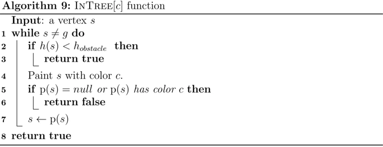
(38) as shown in Algorithm 8. This procedure calls algorithm A. The objective of this search is to reconnect to some state in T : the goal function InTree[c](·) returns true when invoked over a state in T and false otherwise. Once a path is returned, we reconnect the current state with T through the path found and then move to the parent of s. The main loop of Algorithm 7 finishes when the agent reaches the goal. The InTree[c] Function. A key component of reconnection search is the InTree[c] function that determines whether or not a state is in T . Our implementation—shown in Algorithm 9—follows the parent pointers of the state being queried and returns true when it reaches the goal state or a state whose h-value is smaller than hobstacle . This last condition exploits the fact that the way T is built (i.e.: the free-space assumption) ensures that all states that are closer to the goal than all observed obstacles must still be in T . This is merely an optimization technique, and removing it will incur in a small performance reduction, but no change in the actions of the agent. In addition, it paints each visited state with a color c, given as a parameter. The algorithm returns false if a state visited does not have a parent or has been painted with c (i.e., it has been visited before by some previous call to InTree[c] while in the same reconnection search). Algorithm 9: InTree[c] function Input: a vertex s 1 while s 6= g do 2 if h(s) < hobstacle then 3 return true. 6. Paint s with color c. if p(s) = null or p(s) has color c then return false. 7. s. 4 5. 8. p(s). return true Figure 2.1 shows an example execution of the algorithm in an a priori unknown. grid pathfinding task. As can be observed, the agent is moved until a wall is encountered, and then continues bordering the wall until it solves the problem. It is simple 26.

(39) to see that, had the vertical been longer, the agent would have traveled beside the wall following a similar down-up pattern. This example reflects a general behavior of this algorithm in grid worlds: the agent usually moves around obstacles, in a way that resembles bug algorithms (LaValle, 2006; Taylor & LaValle, 2009). This occurs because the agent believes there is a path behind the wall currently known and always tries to move to such a state unless there is another state that allows reconnection and that is found before. A closer look shows that some times the agent does not walk exactly besides the wall but moves very close to them performing a sort of zig-zag movement. This can occur if the search used does not consider the cost of diagonals. Breadth-First Search (BFS) or Depth-First Search (DFS) may sometimes prefer using two diagonals instead of two edges with cost 1. To avoid this problem we can use a variant of BFS, that, for a few iterations, generates first the non-diagonal successors and later the diagonal ones. For nodes deeper in the search it uses the standard ordering (e.g., clockwise). Such a version of BFS achieves in practice a behavior very similar to a bug algorithm.1 This approach was explored in previous work (Rivera, Illanes, et al., 2013), and the overall improvements were shown to be small. For this paper, we use standard BFS. See Section 2.7.2 for a more detailed comparison to bug algorithms. Note that our algorithm does not perform any kind of update to the heuristic h. This contrasts with traditional real-time heuristic search algorithms, which rely on increasing the heuristic value of the h to exit the heuristic depressions generated by obstacles. In such a process they may need to revisit the same cell several times.. 2.4. Satisfying the Real-Time Property FRIT, as presented, does not satisfy the real-time property. There are two reasons for this: 1. Videos can be viewed at http://web.ing.puc.cl/~jabaier/index.php?page=research.. 27.

(40) 1. 2. 3. 4. 5. 6. A. 7. 8. 1. 2. 3. 4. 5. 6. 7. A. 8. 1. 2. 3. 4. 5. 6. 7. 8. A. 1. B. B. B. B. C. C. C. C. D. D. E. E. F. F. (a). D g. 3. 4. 5. 6. 7. 8. D. E. g. F. (b). 2. A. E. g. F. (c). (d). Figure 2.1. An illustration of some of the steps of an execution over a 4-connected grid pathfinding task, where the initial state is cell D3, and the goal is E6. The search algorithm A is breadth-first search, which, when expanding a cell, generates the successors in clockwise order starting with the node to the right. The position of the agent is shown with a black dot. (a) shows the true environment, which is not known a priori by the agent. (b) shows the p pointers which define the ideal tree built initially from the Manhattan heuristic. Following the p pointers, the algorithm leads the agent to D4, where a new obstacle is observed. D5 is disconnected from T and GM , and a reconnection search is initiated. (c) shows the status of T after reconnection search expands state D4, finding E4 is in T . The agent is then moved to E4, from where a new reconnection search expands the gray cells shown in (d). The problem is now solved by simply following the p pointers.. R1. the number of states expanded by a call to the algorithm passed as a parameter, A, depends on the search graph GM rather than on a constant; and, R2. during the execution of A, each time A checks whether or not a state is connected to the ideal tree T , function InTree[c] may visit a number of states dependent on the size of the search graph GM . Below we present two natural approaches to making FRIT satisfy the real-time property. The first approach is to use a slightly modified, generic real-time heuristic search algorithm as a parameter to the algorithm. The resulting algorithm is a realtime search algorithm both because it satisfies the real-time property and because the time between movements is bounded by a constant. The second approach limits the amount of reconnection search but does not guarantee that the time between movements is limited by a constant. 28.

(41) 2.4.1. FRIT with Real-Time Heuristic Search Algorithms A natural way of addressing R1 is by using a real-time search algorithm as parameter to FRIT. It turns out that it is not possible to plug into FRIT a real-time search algorithm directly without modifications. However, the modifications we need to make to Algorithm 5 are simple. We describe them below. The following two observations justify the changes that need to be made to the pseudocode of the generic real-time search algorithm. First we observe that the objective of the lookahead search procedure of real-time heuristic algorithms like Algorithm 5 is to search towards the goal and thus the heuristic h estimates the distance to the goal. However, FRIT carries out search with the sole objective of reconnecting with the ideal tree, which means that both the goal condition and the heuristic have to be changed. Second, one of the main ideas underlying FRIT is to use and maintain the ideal tree T ; that is, when the agent has found a reconnecting path, the p function needs to be updated accordingly. Algorithm 10 shows the pseudocode for the modified generic real-time heuristic search algorithm, which has two main di↵erences with respect to Algorithm 5. First, the goal condition is now given by function gT , which returns true if evaluated with a state that is in T . Second, Line 5 of Algorithm 10 connects the states in the path found by the lookahead search to T . This implies also that the Reconnect procedure described in Algorithm 8 needs to be changed by that described in Algorithm 11. Now we turn our attention to how we can guide the search towards reconnection using reconnecting heuristics. Before giving a formal definition for these heuristics, we introduce a little notation. Given the graph GM = (S, A) and the ideal tree T for GM over a problem P with goal state g, we denote by ST the subset of states in S that are connected to g via arcs in T . Now we are ready to define reconnecting heuristics formally.. 29.

(42) Algorithm 10: A Generic Real-Time Search Algorithm for FRIT Input: A search graph GM , a heuristic function h, a goal function gT (·) that receives a state as parameter. E↵ect: The agent is moved from the initial state to a goal state if a trajectory exists. The ideal tree T is updated. 1 while the agent has not reached a goal state do 2 scurr the current state 3 path LookAhead(scurr , gT (·)) 4 Update the heuristic function h. 5 Given path = s0 s1 . . . sn , update T so that p(si ) = si+1 for every i 2 {0, . . . , n 1}. 6 Move the agent through the path. While moving, observe the environment and update GM and T , removing any non traversable arcs and updating hobstacle if needed. Stop if the current state has no parent in T. Algorithm 11: Reconnect component for FRIT with a real-time algorithm Input: A real-time search algorithm A, an initial state s, a search graph GM and a goal function fGOAL (·) 1 Call A(s, GM , fGOAL ). Definition 2 (Reconnecting Heuristic). Given an ideal tree T over graph GM. and a subset B of ST , we say function h : S ! R+ 0 is a reconnecting heuristic with respect to B i↵ for every s 2 S it holds that h(s)  dGM (s, s0 ), for any s0 2 B.. Intuitively, a reconnecting heuristic with respect to B is an admissible heuristic over the graph GM where the set of goal states is defined as B. As such, when Algorithm 10 is initialized with a reconnecting heuristic, search will be guided towards those connected states. Depending on how we choose B, we may obtain a di↵erent heuristic. At first glance, it may seem sensible to choose B as ST . However, it is not immediately obvious how one would maintain (i.e., learn) such a heuristic efficiently. This is because both T and ST change when new obstacles are discovered. Initially ST contains all states but during execution, some states in S cease to belong to ST as an arc is removed and other become members after reconnection is completed. 30.

(43) In this paper we propose to use an easy-to-maintain reconnecting heuristic, which, for all s is initialized to zero and then is updated in the standard way. Below, we prove that if the update procedure has standard properties, such an h corresponds to a reconnecting heuristic for the subset B = V (E) of ST , where V (E) is defined as follows: B = V (E) = {s 2 ST : s has not been visited by the agent and s 62 E}. In addition, E must be set to the set of states whose heuristic value has been potentially updated by the real-time search algorithm. The reason for this is that, by definition, all states in B should have their h-value set to zero and thus we do not want to include in B states that have been potentially modified. Now we prove that a simple heuristic initialized as 0 for all states and updated in a standard way is indeed a reconnecting heuristic. Proposition 1. Let FRIT be modified to initialize h as the null heuristic. Let E be defined as the set of states that the update procedure has potentially updated.2 Furthermore, assume that A is an instance of Algorithm 10 satisfying: P1. gT (s) returns true i↵ s 2 ST . P2. Heuristic learning maintains consistency; i.e., if h is consistent prior to learning, then it remains as such after learning. Then, along the execution of FRIT(A), h is a reconnecting heuristic with respect to B = V (E). Proof. First we observe that initially h is a reconnecting heuristic because it is set to the zero for every state. Let s be any state in S and s0 be any state in B. We prove that h(s)  d(s, s0 ). Indeed, let. = s0 s1 . . . sn , with s0 = s and sn = s,. 2. Note that in practice, E is a very natural set of states. For example if RTAA* is used, the set of states that have potentially been updated are those that were expanded by some A* lookahead search.. 31.

(44) be a shortest path between s and s0 . Since h is consistent, it holds that h(si )  c(si , si+1 ) + h(si+1 ), for any i 2 {0, . . . , n h(s). (2.1). 1}. From where we can write 0. h(s ) =. n 1 X i=0. h(si ). h(si+1 ) . n 1 X. c(si , si+1 ) = d(s, s0 ). (2.2). i=0. Now observe that because s0 2 B, then the h-value of s0 could have not been updated by the algorithm and therefore h(s0 ) = 0, which substituted in Inequation 2.2, proves the desired result.. ⇤. 2.4.1.1. Tie-breaking In pathfinding, the standard approach to tie-breaking among states with equal f-values is to select the state with highest g-value. For the reconnection search, we propose a di↵erent strategy based on selecting a state based on a user-given heuristic that should guide towards the final goal state. For example, in our experiments on grids we break ties by selecting the state with smallest octile distance to the goal. Intuitively, among two otherwise equal states, we prefer the one that seems to be closer to the final goal. This seems like a reasonable way to use information that is commonly used by other search algorithms, but unavailable to the reconnection search due to the initial use of the null heuristic. 2.4.1.2. Making InTree[c] Real-Time Above we identified R1 and R2 as the two reasons why FRIT does not satisfy the real-time property, and then discussed how to address R1 by using a real-time search algorithm. Now we discuss how to address R2. To address R2, we simply make InTree[c] a bounded algorithm. All real-time search algorithms receive a parameter that allows them to bound the computation carried out per search. Assume that Algorithm 10 receives k as parameter. Furthermore, assume without loss of generality that lookahead search is implemented 32.

(45) with an algorithm that constantly expands states (such as bounded A*). Then we can always choose implementation-specific constants NE and NT , associated respectively to the expansions performed during lookahead and the operation that follows the p pointer in the InTree[c] function. Given that e is the number of expansions performed by lookahead search and f is the number of times the p pointer has been followed in a run of the real-time search algorithm, we modify the stop condition of InTree[c] to return false if NE · e + NT · f > k. Also, we modify lookahead search to stop if the same condition holds true. Henceforth we call FRITRT the algorithm that addresses R1 and R2 using a real-time search algorithm and a bounded version of InTree[c]. Note that because the computation per iteration of FRITRT is bounded, the time between agent moves is bounded, and thus FRITRT can be considered a standard real-time algorithm, as originally defined by Korf (1990). 2.4.2. FRIT with Bounded Complete Search Algorithms In the previous section we proposed to use a standard real-time heuristic search algorithm to reconnect with the ideal tree. A potential downside of such an approach is that those algorithms usually find suboptimal solutions and sometimes require to re-visit the same state many times—a behavior usually referred to as “scrubbing” (Bulitko et al., 2011). In applications in which the quality of the solution is important, but in which there are still real-time constraints it is possible to make FRIT satisfy the real-time property in a di↵erent way. Imagine for example, that we are in a situation in which FRIT is given a sequence of time frames, each of which is very short. After each time frame FRIT is allowed to return a movement which is performed by the agent. Such a model for realtime behavior has been termed as the game time model (Hernández, Baier, Uras, & Koenig, 2012b) since it has a clear application to video games in which the game’s main cycle will reserve a fixed and usually short amount of time to plan the next move for each of the automated characters. 33.

(46) To accommodate this behavior in FRIT we can apply the same simple idea already described in Section 2.4.1.2, but using a complete search algorithm for reconnection rather than a real-time search algorithm. As described above this simply involves choosing implementation-specific constants NE and NT , associated respectively to the expansions performed by the (now complete) search algorithm for reconnection and the operation that follows the p pointer in the InTree[c] function. As before, given that e is the number of expansions performed by reconnection search and f is the number of times the p pointer we modify the Reconnect algorithm to return an empty path as soon as NE e + NT f > k and save all local variables used by A and InTree[c]. Once Reconnect is called again, search is resumed at the same point it was in the previous iteration and e and f are set to 0. Note that instead of returning an empty path other implementations may choose to move the agent in a fashion that is meaningful for the specific application. We leave a thorough discussion on how to implement such a movement strategy out of the scope of this paper since we believe that such a strategy is usually applicationspecific. If a movement ought to be carried out after each time frame, the agent could choose to move back-and-forth, or choose any other moving strategy that allows it to follow the reconnection path once it is found. Later, in our experimental evaluation, we choose not to move the agent if computation exceeds the parameter and discuss why this seems a good strategy in the application we chose. Note that if a non-empty path is returned after each given time frame, then FRIT, modified in the way described above, is also a real-time search algorithm, as originally defined by Korf (1990). Finally, we note that implementing the stop-andresume mechanism described above is easy for most search algorithms.. 2.5. Theoretical Analysis The results described in this section prove the termination of the algorithms and present explicit bounds on the number of agent moves performed by FRIT 34.