TítuloParallel simulation of Brownian dynamics on shared memory systems with OpenMP and Unified Parallel C

Texto completo

(1)1 2 3 4 5 6 7 8 9 10 11 12 13 14 15 16 17 18 19 20 21 22 23 24 25 26 27 28 29 30 31 32 33 34 35 36 37 38 39 40 41 42 43 44 45 46 47 48 49 50 51 52 53 54 55 56 57 58 59 60 61 62 63 64 65. Noname manuscript No. (will be inserted by the editor). Parallel simulation of Brownian dynamics on shared memory systems with OpenMP and Unified Parallel C Carlos Teijeiro · Godehard Sutmann · Guillermo L. Taboada · Juan Touriño. Received: date / Accepted: date. Abstract The simulation of particle dynamics is an essential method to analyze and predict the behavior of molecules in a given medium. This work presents the design and implementation of a parallel simulation of Brownian dynamics with hydrodynamic interactions for shared memory systems using two approaches: (1) OpenMP directives and (2) the Partitioned Global Address Space (PGAS) paradigm with the Unified Parallel C (UPC) language. The structure of the code is described, and different techniques for work distribution are analyzed in terms of efficiency, in order to select the most suitable strategy for each part of the simulation. Additionally, performance results have been collected from two representative NUMA systems, and they are studied and compared against the original sequential code. Keywords Brownian dynamics · parallel simulation · OpenMP · PGAS · UPC · shared memory 1 Introduction Particle based simulation methods have been continuously used in physics and biology to model the behavior of different elements (e.g., molecules, cells) in a medium (e.g., fluid, gas) under thermodynamical conditions (e.g., temperature, density). These methods represent a simplification of the real-world C. Teijeiro, G. L. Taboada, J. Touriño Computer Architecture Group, University of A Coruña 15071 A Coruña, Spain E-mail: {cteijeiro,taboada,juan}@udc.es G. Sutmann Jülich Supercomputing Centre (JSC), Institute for Advanced Simulation Forschungszentrum Jülich GmbH 52425 Jülich, Germany ICAMS, Ruhr-University Bochum, D-44801 Bochum, Germany E-mail: g.sutmann@fz-juelich.de.

(2) 1 2 3 4 5 6 7 8 9 10 11 12 13 14 15 16 17 18 19 20 21 22 23 24 25 26 27 28 29 30 31 32 33 34 35 36 37 38 39 40 41 42 43 44 45 46 47 48 49 50 51 52 53 54 55 56 57 58 59 60 61 62 63 64 65. 2. Carlos Teijeiro et al.. scenario but often provide enough details to model and predict the state and evolution of a system on a given time and length scale. Among them, Brownian dynamics describes the movement of particles in solution on a diffusive time scale, where the solvent particles are taken into account only by their statistical properties, i.e. the interactions between solute and solvent are modeled as a stochastic process. The main goal of this work is to provide a clear and efficient parallelization for the Brownian dynamics simulation, using two different approaches: OpenMP and the PGAS paradigm. On the one hand, OpenMP facilitates the parallelization of codes by simply introducing directives (pragmas) to create parallel regions in the code (with private and shared variables) and distribute their associated workload between threads. Here the access to shared variables is concurrent for all threads, thus the programmer should control possible data dependencies and deadlocks. On the other hand, PGAS is an emerging paradigm that treats memory as a global address space divided in private and shared areas. The shared area is logically partitioned in chunks with affinity to different threads. Using the UPC language [15] (which extends ANSI C including PGAS support) the programmer can deal directly with workload distribution and data storage by means of different constructs, such as assignments to shared variables, collective functions or parallel loop definitions. The rest of the paper presents the design and implementation of the parallel code. First, some related work on this area is presented, and then a mathematical and computational description of the different parts in the sequential code is provided. Next, the most relevant design decisions taken for the parallel implementation of the code, according to the nature of the problem, are discussed. Finally, a performance analysis of the parallel code is accomplished, and the main conclusions are drawn.. 2 Related work There are multiple works on simulations based on Brownian dynamics, e.g. several simulation tools such as BrownDye [7] and the BROWNFLEX program included in the SIMUFLEX suite [5], and many other studies oriented to specific fields, such as DNA research [8] or copolymers [10]. Although most of these works focus on sequential codes, some of them have developed parallel implementations with OpenMP, applied to smoothed particle hydrodynamics (SPH) [6] and the transportation of particles in a fluid [16]. The UPC language has also been used in a few works related to particle simulations, such as the implementation of the particle-in-cell algorithm [12]. However, comparative analyses between parallel programming approaches on shared memory with OpenMP and UPC are mainly restricted to some computational kernels for different purposes [11,17], without considering large simulation applications. The most relevant recent work on parallel Brownian dynamics simulation is BD BOX [2], which supports simulations on CPU using codes written with MPI and OpenMP, and also on GPU with CUDA. However, there is still little.

(3) 1 2 3 4 5 6 7 8 9 10 11 12 13 14 15 16 17 18 19 20 21 22 23 24 25 26 27 28 29 30 31 32 33 34 35 36 37 38 39 40 41 42 43 44 45 46 47 48 49 50 51 52 53 54 55 56 57 58 59 60 61 62 63 64 65. Parallel Brownian dynamics on shared memory. 3. information published about the actual algorithmic implementation of these simulations, and their performance has not been thoroughly studied, especially under periodic boundary conditions. In order to solve this and provide an efficient parallel solution on different NUMA shared memory systems, we have analyzed the Brownian dynamics simulation for different problem sizes, and described how to address the main performance issues of the code using OpenMP and a PGAS-based approach with UPC.. 3 Theoretical description of the simulation The present work focuses on the simulation of Brownian motion of particles including hydrodynamic interactions. The time evolution in configuration space has been stated by Ermak and McCammon [3] (based on the Focker-Planck and Langevin descriptions) which includes the direct interactions between particles via systematic forces as well as solvent mediated effects via a correlated random process ri (t + ∆t) = ri (t) +. ! ∂Dij (t) j. ∂rj. ∆t +. ! j. 1 Dij (t)Fj (t)∆t + Ri (t + ∆t) (1) kB T. Here the underlying stochastic process can be discretized in different ways, leading to e.g. the Milstein [9] or Runge-Kutta [14] schemes, but in Eq. 1 the time integration method follows a simple Euler scheme. In a system that contains N particles, the trajectory {ri (t); t ∈ [0, tmax ]} of particle i is calculated as a succession of small and fixed time step increments ∆t, defined as the sum of interactions on the particles during each time step (that is, the partial derivative of the initial diffusion tensor D0ij with respect to the position component and the product of the forces F and the diffusion tensor at the beginning of a time step, being kB Boltzmann’s constant and T the absolute temperature), and a random displacement Ri (∆t) associated to the possible correlations between displacements for each particle. The random displacement vector R is Gaussian distributed with average value "Ri # = 0 and covariance "Ri (t + ∆t)RTj (t + ∆t)# = 2Dij (t)∆t. The diffusion tensor D thereby contains information about hydrodynamic interactions, which, formally, can be neglected by considering only the diagonal components Dii . Choosing appropriate models for the diffusion tensor, the partial derivative of D drops out of Eq. 1, which is true for the Rotne-Prager tensor [13] used in this work. Therefore, Eq. 1 reduces to ∆r =. √ 1 DF∆t + 2∆t S ξ kT. (2). √ where the expression R = 2∆tSξξ holds and D = SST , which relates the stochastic process to the diffusion matrix. Therefore, S may be calculated via a Cholesky decomposition of D or via the square root of D. Both approaches are very CPU time consuming and have a complexity of O(N 3 ). A faster approach.

(4) 1 2 3 4 5 6 7 8 9 10 11 12 13 14 15 16 17 18 19 20 21 22 23 24 25 26 27 28 29 30 31 32 33 34 35 36 37 38 39 40 41 42 43 44 45 46 47 48 49 50 51 52 53 54 55 56 57 58 59 60 61 62 63 64 65. 4. Carlos Teijeiro et al.. that approximates the random displacement vector R without constructing S explicitly was introduced by Fixman [4] using an expansion of R in terms of Chebyshev polynomials, which has a complexity of O(N 2.25 ). The interaction model for the computation of forces in the system (which here considers periodic boundary conditions) consists of (1) direct systematic interactions, which are computed as Lennard-Jones type interactions and evaluated within a fixed cutoff radius, and (2) hydrodynamic interactions, which have long range character. The latter ones are reflected in the off-diagonal components of the diffusion tensor D and therefore contribute to both terms of the right-hand side of Eq. 2. Due to the long range nature, the diffusion tensor is calculated via the Ewald summation method [1]. 4 Design of the parallel simulation The sequential code considers a unity 3-dimensional box with periodic boundary conditions that contains a set of N equal particles. The main part of this code is a for loop in which each iteration represents a time step. Following the formulas presented in Section 3, each time step of the simulation consists of two main parts: (1) the calculation of the forces that act on each particle (function calc force), and (2) the computation of random displacements for every particle in the system (function covar). The main loop of time steps is not parallelizable, as each iteration depends on the previous one. However, the workload of each iteration can be executed in parallel through a domain decomposition of the work. Here OpenMP requires separate parallel regions for each function, as a work distribution is only possible if the parallel region is defined inside the target function; otherwise, its arguments would be treated mandatorily as private variables. Nevertheless, UPC targets a balanced workload distribution between threads and an efficient data access, exploiting the NUMA architecture through the maximization of data locality (processing the data stored in the thread’s affine space). A more detailed description of both OpenMP and UPC parallelizations is given in the next subsections. 4.1 Calculation of interactions The main part of the computation in function calc force consists in updating the diffusion tensor D, which is defined in the code as a symmetric square pNDIM×pNDIM matrix (called D), where pNDIM= 3 × N (that is, one value per dimension and per pair of particles). For each element in matrix D, the Ewald summation is split into (1) a short range part, where elements are calculated according to pairwise distances within a cutoff radius, and (2) a long range part, which is evaluated in Fourier k-space. Both computations are performed individually for each value in matrix D using the current coordinates for each particle in the system with two separate loops. In the sequential code, these loops operate only on the upper triangular part of D, because of its symmetry..

(5) 1 2 3 4 5 6 7 8 9 10 11 12 13 14 15 16 17 18 19 20 21 22 23 24 25 26 27 28 29 30 31 32 33 34 35 36 37 38 39 40 41 42 43 44 45 46 47 48 49 50 51 52 53 54 55 56 57 58 59 60 61 62 63 64 65. Parallel Brownian dynamics on shared memory. 5. According to the previous definitions, the independent computation of values of matrix D defines a straightforward parallelization for calc force in the simulation. The OpenMP implementation uses an omp for directive to parallelize the computation of short and long range interactions, using a dynamic scheduling of iterations because of the different amount of values calculated per particle/dimension, alongside with atomic directives to obtain the average overall speed and pressure values. The UPC code performs an analogous processing, but using a 1D storage for matrix D: its elements are divided in THREADS equal chunks (being THREADS the number of threads in the UPC program), and each thread computes its associated values for each particle for all dimensions.. 4.2 Computation of random displacements The random displacements are calculated for each particle as Gaussian random numbers with prescribed covariances according to the diffusion tensor matrix. The simulation code includes two alternative methods to obtain the covariance terms: (1) a Cholesky decomposition of D and (2) the Fixman’s approximation method. The Cholesky decomposition of matrix D obtains a lower triangular matrix L, whose values for each row are multiplied by a random value generated for the corresponding particle and dimension. The final result is the sum of all these products, as stated in Eq. 3, where row i represents particle i div DIM in dimension i mod DIM (with DIM= 3, the number of dimensions), and xic is the array of pNDIM random values: Ri (t + ∆t) =. i ! j=1. L[i][j] · xic[j]. (3). The original sequential algorithm calculates the first three values of the lower triangular result matrix (that is, the elements of the first two rows), and then the remaining values are computed row by row in a loop. Here the data dependencies between the values in L computed in each iteration and the ones computed in previous iterations prevent the direct parallelization of the loop. However, UPC takes advantage of its data manipulation facilities and computes the values in L as a sum (reduction) of different contributions calculated by each thread: after a row in matrix L is computed, its elements are used to obtain partial computations of the random displacements associated to the unprocessed rows, thus maximizing parallelism. This functionality is implemented in UPC using the upc forall construct to distribute the loop iterations between threads, and a broadcast collective to send partial computations. Listing 1 presents a pseudocode of this algorithm. Regarding OpenMP, and given the difficulties for an efficient parallelization of the original algorithm commented previously, an alternative iterative algorithm is proposed: the first column of the result matrix is calculated by.

(6) 1 2 3 4 5 6 7 8 9 10 11 12 13 14 15 16 17 18 19 20 21 22 23 24 25 26 27 28 29 30 31 32 33 34 35 36 37 38 39 40 41 42 43 44 45 46 47 48 49 50 51 52 53 54 55 56 57 58 59 60 61 62 63 64 65. 6. Carlos Teijeiro et al. f o r e v e r y row ‘ i ’ i n m a tr i x D i f th e row i s a s s i g n e d to MYTHREAD o b t a i n v a l u e s o f row ‘ i ’ i n L c a l c u l a t e random d i s p l a c e m e n t ‘ i ’ endif b r o a d c a s t v a l u e s i n row ‘ i ’ to a l l t h r e a d s u p c f o r a l l rows ‘ j ’ l o c a t e d a f t e r ‘ i ’ i n m a tr i x D c a l c u l a t e p a r t i a l v a l u e s f o r e l e m e n t s i n row ‘ j ’ c a l c u l a t e p a r t i a l value f o r displacement ‘ j ’ endfor endfor. Listing 1 UPC pseudocode for Cholesky decomposition. dividing the values of the first row in the source matrix by its diagonal value (parallelizable for loop), then these values are used to compute a partial contribution to the rest of elements in the matrix (also parallelizable for loop). Finally, these two steps are repeated to obtain the rest of columns in the result matrix. Listing 2 shows the source code of the iterative algorithm: a static scheduling is used in the first two loops, whereas the last two use a dynamic one because of the different workload associated to their iterations. L [ 0 ] [ 0 ] = s q r t (D [ 0 ] [ 0 ] ) ; #pragma omp p a r a l l e l p r i v a t e ( i , j , k ) { #pragma omp f o r s c h e d u l e ( s t a t i c ) f o r ( j =1; j <N∗DIM ; j ++) L[ j ] [ 0 ] = D[ 0 ] [ j ]/L [ 0 ] [ 0 ] ; #pragma omp f o r s c h e d u l e ( s t a t i c ) f o r ( j =1; j <N∗DIM ; j ++) f o r ( k =1; k<=j ; k++) L [ j ] [ k ] = D[ k ] [ j ]−L [ 0 ] [ j ] ∗ L [ 0 ] [ k ] ; f o r ( i =1; i <N∗DIM ; i ++) { L [ i ] [ i ] = s q r t (L [ i ] [ i ] ) ; #pragma omp f o r s c h e d u l e ( dynamic ) f o r ( j=i +1; j <N∗DIM; j ++) L [ j ] [ i ] = L[ i ] [ j ] /L [ i ] [ i ] ; #pragma omp f o r s c h e d u l e ( dynamic ) f o r ( j=i +1; j <N∗DIM; j ++) f o r ( k=i +1; k<=j ; k++) L [ j ] [ k ] −= L [ i ] [ j ] ∗ L [ i ] [ k ] ; } } Listing 2 Iterative Cholesky decomposition with OpenMP. Fixman’s algorithm [4] is an alternative to Cholesky decomposition to obtain the covariance terms of random displacements. This method approximates R using the Chebyshev polynomial SMξ , where SM is an approximation to.

(7) 1 2 3 4 5 6 7 8 9 10 11 12 13 14 15 16 17 18 19 20 21 22 23 24 25 26 27 28 29 30 31 32 33 34 35 36 37 38 39 40 41 42 43 44 45 46 47 48 49 50 51 52 53 54 55 56 57 58 59 60 61 62 63 64 65. Parallel Brownian dynamics on shared memory. 7. S (cf. Eq. 2) and the number of polynomial coefficients M controls the accuracy of the approximation, without constructing an additional matrix as with Cholesky decomposition. Practically this algorithm works on a scaled matrix, with eigenvalues within the range λ ∈ [−1, 1], thus requiring to know the smallest (λmin ) and largest (λmax ) eigenvalues of matrix D, as stated in Eq. 4. L ! √ d≈ al Cl , where L ≡ order of the polynomial approximation, and l=0. C0 = 1 ; C1 = da d + db ; Cl+1 = 2(da d + db )Cl − Cl−1 , having (4) 2 λmax + λmin da = ; db = λmax − λmin λmax − λmin According to this, two iterative approximation methods are used for Fixman’s algorithm: (1) the calculation of the minimum and maximum eigenvalues of matrix D, which uses a variant of the power method, and (2) the computation of covariance terms following the formulas in Eq. 4. In both cases, the core of the algorithm consists of two for loops that operate on every row of matrix D independently (thus fully parallelizable) until the predefined accuracy is reached. Each iteration of these methods requires all the approximations computed for every particle in all dimensions (pNDIM values) in the previous iteration, thus both codes use two arrays that are read or written alternatively on each iteration to avoid additional data copies. The OpenMP code includes omp for directives for each loop to compute approximations, using a critical directive to obtain the maximum/minimum eigenvalues of D and a reduction clause to compute the total error value for the final approximated covariance terms. Listing 3 presents the pseudocode of the loop that computes the maximum eigenvalue of D, using x and x d as working arrays for the iterative method. Here a reduction clause with a maximum operator could be used instead of the critical directive, but in this case the experimental analysis showed better performance using critical. The UPC parallelization requires the use of three collective operations (all-to-all, allgather and allreduce) to obtain the final results of both iterative methods. A prototypical implementation of their associated loops is shown in Listing 4, where the approximations are stored alternatively in arrays x and x d, as in the code in Listing 3. Each thread computes a partial result for the approximated eigenvalues in its local memory, and then an all-to-all collective communication is performed to get all the partial results of their assigned particles. After that, each thread obtains an approximation of its associated maximum eigenvalue, and finally an allgather collective ensures that all threads have all the approximated values in order to prepare a new iteration of the approximation method. At the end of the while loop, the maximum eigenvalue is obtained with a reduction of the partial values computed on each thread. In general terms, the presented UPC parallelization required additional lines of source code (SLOCs) than using OpenMP. This is due to the data.

(8) 1 2 3 4 5 6 7 8 9 10 11 12 13 14 15 16 17 18 19 20 21 22 23 24 25 26 27 28 29 30 31 32 33 34 35 36 37 38 39 40 41 42 43 44 45 46 47 48 49 50 51 52 53 54 55 56 57 58 59 60 61 62 63 64 65. 8. Carlos Teijeiro et al. #pragma omp p a r a l l e l { w h i l e th e r e q u i r e d a c c u r a c y f o r ‘ eigmax ’ i s not r e a c h e d do i f th e i t e r a t i o n number i s even // r e a d from ‘ x ’ , w r i t e to ‘ x d ’ #pragma omp f o r s c h e d u l e ( s t a t i c ) \ def aul t ( shared ) pr i vate ( i , j , . . . ) f o r e v e r y p a r t i c l e ‘ i ’ i n th e system x d [ i ] = 0; f o r e v e r y p a r t i c l e ‘ j ’ i n th e system x d [ i ] += D[ i ] [ j ] ∗ x [ j ] / eigmax ; endfor #pragma omp c r i t i c a l i f i t i s th e maximum v a l u e s e l e c t i t i n ‘ eigmax ’ endif endfor else // The same code a s above , but c h a n g i n g // ‘ x ’ with ‘ x d ’ and v i c e v e r s a endif endwhile }. Listing 3 OpenMP pseudocode that computes the maximum eigenvalue of matrix D. movements, especially collective operations, that are needed for an efficient access to the data set (logically stored in the thread’s shared and private memory spaces). However, thanks to these data movement operations, the UPC code can take advantage of efficient data layouts both for NUMA and distributed memory systems [11]. This higher flexibility of UPC contrasts with the limitation of UPC collectives, which can only be used on 1D arrays and thus the code was adapted accordingly, as mentioned at the end of Section 4.1. Regarding OpenMP, the parallelization was mainly accomplished by introducing directives in the source code, but this code also required major changes in order to obtain scalability (as it was the case for Cholesky decomposition).. 5 Performance evaluation Two different NUMA systems have been used for the performance analysis. The first one (named NEH in the graphs) consists of 2 Intel Xeon X5570 (Nehalem-EP) quad-core processors at 2.93 GHz with Simultaneous Multithreading (SMT) and 24 GB of memory at 1066 MHz. The second system (MGC) is an HP ProLiant SL165z G7 node with 2 dodeca-core AMD Opteron processors 6174 (Magny-Cours) at 2.2 GHz with 32 GB of memory. The Intel C Compiler (icc) v12.1 and the Open64 Compiler Suite (opencc) v4.2.5.2 have been used as OpenMP compilers in NEH and MGC, respectively. The UPC compiler in both systems is Berkeley UPC 2.14.2 (a UPC-to-C source-to-source compiler) with the SMP conduit, backed by the aforementioned C compilers.

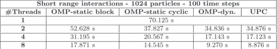
(9) 1 2 3 4 5 6 7 8 9 10 11 12 13 14 15 16 17 18 19 20 21 22 23 24 25 26 27 28 29 30 31 32 33 34 35 36 37 38 39 40 41 42 43 44 45 46 47 48 49 50 51 52 53 54 55 56 57 58 59 60 61 62 63 64 65. Parallel Brownian dynamics on shared memory. 9. w h i l e th e r e q u i r e d a c c u r a c y f o r ‘ eigmax ’ i s not r e a c h e d do i f th e i t e r a t i o n number i s even // r e a d from ‘ x ’ , w r i t e to ‘ x d ’ f o r e v e r y el em en t i n ‘D’ ( a s s o c i a t e d to each t h r e a d ) compute p a r t i a l a p p r o x i m a ti o n i n ‘ copyArray ’ u s i n g ‘ x ’ endfor a l l −to− a l l c o l l e c t i v e to g e t a l l p a r t i a l \ a p p r o x i m a t i o n s from ‘ copyArray ’ f o r every p a r t i c l e ‘ i ’ i n th e system f o r e v e r y ‘THREADS’ p a r t i a l r e s u l t s i n ‘ copyArray ’ sum p a r t i a l r e s u l t s to g e t th e f i n a l \ a p p r o x i m a ti o n o f ‘ x d [ i ] ’ endfor i f i t i s th e maximum v a l u e s e l e c t i t i n ‘ eigmax ’ endif endfor g a t h e r a l l th e computed v a l u e s i n ‘ x d ’ else // The same code a s above , but c h a n g i n g // ‘ x ’ with ‘ x d ’ and v i c e v e r s a endif r e d u c e a l l th e ‘ eigmax ’ v a l u e s on each t h r e a d endwhile Listing 4 UPC pseudocode that computes the maximum eigenvalue of matrix D. on each system. The optimization flags used in all executions are -fast for icc and -Ofast for opencc. The environment variable OMP STACKSIZE has been set to a small value (128 KB) for OpenMP executions in order to obtain the highest efficiency. Periodic boundary conditions (3×3 boxes per dimension) are considered for all simulations. Next some relevant performance results of specific parts of the code (Tables 1-3) are detailed, and after them Figures 1 and 2 show data of the whole simulation. Table 1 Execution time profile of the sequential code Code Part calc force - short range contributions calc force - long range contributions covar - option 1: Cholesky covar - option 2: Fixman move Total time (with Cholesky) Total time (with Fixman). 128 particles 1.104 2.954 0.838 0.265 0.006. 1024 particles. s s s s s. 70.125 s 522.867 s 435.748 s 28.327 s 0.483 s. 4.902 s 4.329 s. 1029.223 s 621.802 s. Table 1 shows the execution time breakdown of sequential simulations (128 and 1024 particles with 100 time steps) in the NEH system, considering the functions commented in Section 4 and including the computation of the new coordinates for the next time step as a separate function (called move). These.

(10) 1 2 3 4 5 6 7 8 9 10 11 12 13 14 15 16 17 18 19 20 21 22 23 24 25 26 27 28 29 30 31 32 33 34 35 36 37 38 39 40 41 42 43 44 45 46 47 48 49 50 51 52 53 54 55 56 57 58 59 60 61 62 63 64 65. 10. Carlos Teijeiro et al.. results give a measure of the different weights and algorithmic complexities of 2 each part of the code. As the diffusion tensor matrix D has (3 × N ) elements, 2 its construction has a complexity of at least O(N ), which is related to the computation of short and long range interactions. However, the long range part has an additional contribution because of the use of reciprocal vectors to obtain the required error tolerance in the Ewald sum, which increases its complexity to approximately O(N 2.5 ). Regarding the computation of random displacements (function covar), the results clearly show the effect of the higher complexity of the Cholesky decomposition with respect to Fixman’s algorithm. Table 2 presents performance results of the loop that computes short range interactions (see Section 4.1) in a 1024-particle system with 100 time steps using the NEH system, with initial conditions chosen as a regular grid. These results confirm that the OpenMP dynamic distribution of iterations outperforms the static ones (block and cyclic) because of the different workload associated to each iteration, obtaining about 7.56 of speedup with 8 threads. This speedup is limited by the sequential calculations of pressure and speed using the atomic directive, which creates a lightweight critical section that solves the data dependencies. The UPC version obtains similar results (slightly better for 8 threads) to the most efficient OpenMP implementation.. Table 2 Execution times of short range interactions with OpenMP and UPC Short range interactions - 1024 particles - 100 time steps #Threads OMP-static block OMP-static cyclic OMP-dyn. 1 70.125 s 2 52.628 s 37.827 s 34.836 s 4 31.195 s 20.567 s 17.143 s 8 17.871 s 14.545 s 9.270 s. UPC 34.876 s 17.123 s 8.876 s. Table 3 presents the results of OpenMP and UPC Cholesky decomposition algorithms (see Section 4.2) using 1024 particles with 100 time steps on NEH, which shows that the original implementation (used in UPC) is the most efficient sequential routine. Even though the OpenMP iterative version obtains scalability up to 8 threads, it is far from the ideal because of loop i presented in Listing 2: implicit synchronizations executed at the end of each nested loop j due to the omp for directive, thus involving a significant overhead.. Table 3 Execution times of covar using Cholesky with 1024 particles and 100 time steps Code \ #Threads OpenMP UPC. 1 568.153 s 435.748 s. 2 396.564 s 345.924 s. 4 354.792 s 250.175 s. 8 348.334 s 182.432 s.

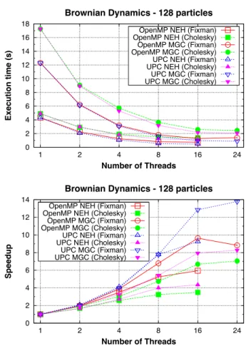
(11) Parallel Brownian dynamics on shared memory. 11. Figure 1 presents the execution times and speedups of the whole simulation with 128 particles and 100 time steps. The execution times of NEH are better than those of MGC for both random displacement generation methods, even though the influence of using SMT for 16 threads affects performance. This is mainly due to the higher processor power of NEH. The reduced problem size involves a low average workload per thread, thus the bottlenecks of the code (e.g., OpenMP atomic directives and UPC collective communications) are more noticeable. Nevertheless, the UPC implementation compiled with Berkeley UPC even obtains superlinear speedup for 2 and 4 threads with Fixman on NEH. Regarding the covar function, the use of Fixman’s method clearly helps to obtain higher performance when compared to Cholesky decomposition, as stated in the previous sections.. Brownian Dynamics - 128 particles 18. OpenMP NEH (Fixman) OpenMP NEH (Cholesky) OpenMP MGC (Fixman) OpenMP MGC (Cholesky) UPC NEH (Fixman) UPC NEH (Cholesky) UPC MGC (Fixman) UPC MGC (Cholesky). Execution time (s). 16 14 12 10 8 6 4 2 0 1. 2. 4. 8. 16. 24. Number of Threads. Brownian Dynamics - 128 particles 14 12 10. Speedup. 1 2 3 4 5 6 7 8 9 10 11 12 13 14 15 16 17 18 19 20 21 22 23 24 25 26 27 28 29 30 31 32 33 34 35 36 37 38 39 40 41 42 43 44 45 46 47 48 49 50 51 52 53 54 55 56 57 58 59 60 61 62 63 64 65. 8. OpenMP NEH (Fixman) OpenMP NEH (Cholesky) OpenMP MGC (Fixman) OpenMP MGC (Cholesky) UPC NEH (Fixman) UPC NEH (Cholesky) UPC MGC (Fixman) UPC MGC (Cholesky). 6 4 2 0 1. 2. 4. 8. 16. Number of Threads Figure 1 Performance results with 128 particles (Fixman and Cholesky). 24.

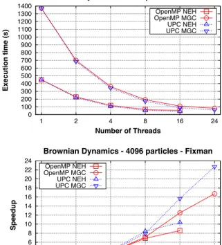
(12) 12. Carlos Teijeiro et al.. Figure 2 shows the simulation results for a large number of particles (4096) and 5 time steps. Only the results of covar with Fixman’s algorithm are shown, because of its higher performance. The results up to 8 threads present similar performance, which is mainly due to the heavy computation of long range interactions compared to the relatively small computation of random displacements. In fact, the larger problem size provides higher speedups than those of Figure 1. However, the algorithmic complexity of calculating the diffusion tensor D is O(N 2 ), whereas Fixman’s algorithm is O(N 2.25 ); thus, when the problem size increases, the generation of random displacements represents a larger percentage of the total simulation time. As a result of this, and also given the parallelization issues commented in Section 4.2, the speedup is slightly limited for 16 or more threads, mainly for OpenMP (also due to the use of SMT in NEH). However, considering the distance to the ideal speedup, we can conclude that both systems present reasonably good speedups for this code.. Brownian Dynamics - 4096 particles - Fixman. Execution time (s). 1400 1300 1200 1100 1000 900 800 700 600 500 400 300 200 100 0. OpenMP NEH OpenMP MGC UPC NEH UPC MGC. 1. 2. 4. 8. 16. 24. Number of Threads. Brownian Dynamics - 4096 particles - Fixman. Speedup. 1 2 3 4 5 6 7 8 9 10 11 12 13 14 15 16 17 18 19 20 21 22 23 24 25 26 27 28 29 30 31 32 33 34 35 36 37 38 39 40 41 42 43 44 45 46 47 48 49 50 51 52 53 54 55 56 57 58 59 60 61 62 63 64 65. 24 22 20 18 16 14 12 10 8 6 4 2 0. OpenMP NEH OpenMP MGC UPC NEH UPC MGC. 1. 2. 4. 8. Number of Threads. Figure 2 Performance results with 4096 particles (Fixman). 16. 24.

(13) 1 2 3 4 5 6 7 8 9 10 11 12 13 14 15 16 17 18 19 20 21 22 23 24 25 26 27 28 29 30 31 32 33 34 35 36 37 38 39 40 41 42 43 44 45 46 47 48 49 50 51 52 53 54 55 56 57 58 59 60 61 62 63 64 65. Parallel Brownian dynamics on shared memory. 13. 6 Conclusions This work has presented the parallel implementation of a Brownian dynamics simulation code on shared memory using OpenMP directives and a PGASbased approach with the UPC language. According to both programming paradigms, different workload distributions have been presented and tested for the main functions in the code, trying to obtain good performance as the number of threads increases. The scheduling techniques in for loops, the convenient use of reduction or critical directives, and the control of the stack size in parallel function calls have been the most relevant features to tune the OpenMP code, whereas the efficient work distribution and a wise optimization of data management have been key factors for UPC. The results of the parallel implementation have shown that there is a high dependency of the code on the part where random displacements are generated for each particle, and here Fixman’s approximation method has shown to be the best choice. Regarding both programming paradigms, UPC has obtained better results than OpenMP, mainly because of the more efficient access to the data set, as the PGAS memory model presents a more straightforward adaptation to current NUMA multicore-based systems, although at the cost of a slightly higher programming effort. OpenMP has provided a more compact implementation in terms of SLOCs and a more straightforward approach to parallel programming but, in general, the trade-off between programmability and performance has been favorable for the UPC code.. Acknowledgements This work was funded by the Ministry of Science and Innovation of Spain (Project TIN2010-16735), the Spanish network CAPAP-H3 (Project TIN201012011-E), and by the Galician Government (Pre-doctoral Program “Marı́a Barbeito” and Program for the Consolidation of Competitive Research Groups, ref. 2010/6).. References 1. Beenakker, C.: Ewald Sum of the Rotne-Prager Tensor. Journal of Chemical Physics 85, 1581–1582 (1986) 2. D!lugosz, M., Zieliński, P., Trylska, J.: Brownian Dynamics Simulations on CPU and GPU with BD BOX. Journal of Computational Chemistry 32(12), 2734–2744 (2011) 3. Ermak, D.L., McCammon, J.A.: Brownian Dynamics with Hydrodynamic Interactions. Journal of Chemical Physics 69(4), 1352–1360 (1978) 4. Fixman, M.: Construction of Langevin Forces in the Simulation of Hydrodynamic Interaction. Macromolecules 19(4), 1204–1207 (1986) 5. Garcı́a de la Torre, J., Hernández Cifre, J.G., Ortega, A., Schmidt, R.R., Fernandes, M.X., Pérez Sánchez, H.E., Pamies, R.: SIMUFLEX: Algorithms and Tools for Simulation of the Conformation and Dynamics of Flexible Molecules and Nanoparticles in Dilute Solution. Journal of Chemical Theory and Computation 5(10), 2606–2618 (2009).

(14) 1 2 3 4 5 6 7 8 9 10 11 12 13 14 15 16 17 18 19 20 21 22 23 24 25 26 27 28 29 30 31 32 33 34 35 36 37 38 39 40 41 42 43 44 45 46 47 48 49 50 51 52 53 54 55 56 57 58 59 60 61 62 63 64 65. 14. Carlos Teijeiro et al.. 6. Hipp, M., Rosenstiel, W.: Parallel Hybrid Particle Simulations Using MPI and OpenMP. In: 10th International Euro-Par Conference (Euro-Par’04), Pisa (Italy), pp. 189–197 (2004) 7. Huber, G.A., McCammon, J.A.: Browndye: A Software Package for Brownian Dynamics. Computer Physics Communications 181(11), 1896 – 1905 (2010) 8. Klenin, K., Merlitz, H., Langowski, J.: A Brownian Dynamics Program for the Simulation of Linear and Circular DNA and Other Wormlike Chain Polyelectrolytes. Biophysical Journal 74(2 Pt 1), 780–788 (1998) 9. Kloeden, P.E., Platen, E.: Numerical Solution of Stochastic Differential Equations. Springer, Berlin (1992) 10. Li, B., Zhu, Y.L., Liu, H., Lu, Z.Y.: Brownian Dynamics Simulation Study on the Self-assembly of Incompatible Star-like Block Copolymers in Dilute Solution. Physical Chemistry Chemical Physics 14, 4964–4970 (2012) 11. Mallón, D.A., Taboada, G.L., Teijeiro, C., Touriño, J., Fraguela, B.B., Gómez, A., Doallo, R., Mouriño, J.C.: Performance Evaluation of MPI, UPC and OpenMP on Multicore Architectures. In: 16th European PVM/MPI Users’ Group Meeting (EuroPVM/MPI’09), Espoo (Finland), pp. 174–184 (2009) 12. Markidis, S., Lapenta, G.: Development and Performance Analysis of a UPC Particlein-Cell Code. In: 4th Conference on Partitioned Global Address Space Programming Models (PGAS’10), New York (NY, USA), pp. 10:1–10:9. ACM (2010) 13. Rotne, J., Prager, S.: Variational Treatment of Hydrodynamic Interaction in Polymers. Journal of Chemical Physics 50(11), 4831–4837 (1969) 14. Tocino, A., Vigo-Aguiar, J.: New Itô–Taylor Expansions. Journal of Computational and Applied Mathematics 158(1), 169–185 (2003) 15. Unified Parallel C at George Washington University: http://upc.gwu.edu. Accessed 31 October 2012 16. Wei, W., Al-Khayat, O., Cai, X.: An OpenMP-enabled Parallel Simulator for Particle Transport in Fluid Flows. In: 11th International Conference on Computational Science (ICCS’11), Singapore, pp. 1475–1484 (2011) 17. Zhao, W., Wang, Z.: ScaleUPC: A UPC Compiler for Multi-core Systems. In: 3rd Conference on Partitioned Global Address Space Programing Models (PGAS’09), Ashburn (VA, USA), pp. 11:1–11:8. ACM (2009).

(15)