Author’s Accepted Manuscript
A useful tool for computation and interpretation of
trading-off solutions through pareto-optimal front in
the field of experimental designs for mixtures
M.S. Sánchez, M.C. Ortiz, L.A. Sarabia
PII:
S0169-7439(16)30323-9
DOI:
http://dx.doi.org/10.1016/j.chemolab.2016.09.007
Reference:
CHEMOM3319
To appear in:
Chemometrics and Intelligent Laboratory Systems
Received date: 4 June 2016
Revised date:
12 September 2016
Accepted date: 18 September 2016
Cite this article as: M.S. Sánchez, M.C. Ortiz and L.A. Sarabia, A useful tool for
computation and interpretation of trading-off solutions through pareto-optimal
front in the field of experimental designs for mixtures,
Chemometrics and
Intelligent
Laboratory
Systems,
http://dx.doi.org/10.1016/j.chemolab.2016.09.007
This is a PDF file of an unedited manuscript that has been accepted for
publication. As a service to our customers we are providing this early version of
the manuscript. The manuscript will undergo copyediting, typesetting, and
review of the resulting galley proof before it is published in its final citable form.
Please note that during the production process errors may be discovered which
could affect the content, and all legal disclaimers that apply to the journal pertain.
Page 1/ 19
A useful tool for computation and interpretation of trading-off solutions
through pareto-optimal front in the field of experimental designs for
mixtures
M.S. Sánchez1, M.C. Ortiz2*, L.A. Sarabia1
1Department of Mathematics and Computation, University of Burgos, Plaza Misael Bañuelos s/n, Burgos, Spain 2Department of Chemistry (Analytical Chemistry), University of Burgos, Plaza Misael Bañuelos s/n, Burgos,
Spain
*Corresponding author. E-mail: [email protected]
Abstract
An algorithmic implementation is presented to deal with several responses in mixtures problems, without theoretical limits on the number of responses or on the factors to be blended. Also, constrained and unconstrained domains are handled, as well as domains with both mixtures and discrete variables. Besides, an alternative way of interpreting the results coming from the experimental design for mixtures is presented. It is based on the parallel coordinates plots for visualization in more than the usual three-dimensional Cartesian diagrams or the simplex mixture spaces for at most four experimental factors.
Specifically, this is done in cases in which more than one experimental response should be handled, tackling the conflict by estimating trading-off solutions via the computation of the pareto-optimal front, which is fully explored with the parallel coordinates plots.
The procedure is shown by two case-studies, taken from the literature. The first one deals with several factors in a constrained experimental domain when trying to optimize a detergent by taking into account two severely conflicting characteristics. The second one is about five chemical components blended with different dosage levels for getting a concrete strong enough, experimental results that are re-evaluated by posing a unique blocked design for analysing the data.
The joint use of the pareto-optimal front for mixtures designs and the parallel coordinates plots for its visualization provide the researcher a deeper understanding of the problem under study to make accurate decisions.
Keywords
Page 2/ 19
1. INTRODUCTION
According to Smith [1], scientific experiments can be sequenced in three stages: planning the experiments, conducting the planned experiments and analysing/interpreting the collected results. Provided at least that the planning involves statistical design of experiments (DOE), the experiments are randomized (blocked if necessary) and the interpretation uses statistical analysis of data, the three stages all together comprise what he call the experimental design process, emphasizing the need of the three phases, despite the fact that, when talking about experimental design process, it seems that it only refers to planning. The present work addresses the three stages, centred in the experimental designs for mixtures, and emphasising the last step: how to interpret the data obtained with the experiments.
When the (experimental) factors to be handled in a given problem are proportions of a blend, we are dealing with specific experimental designs, those for mixtures. One of the distinctive characteristics of experimental designs for mixtures is that their factors are always linearly dependent, because in each experiment the variables should be positive and sum to unity. The usual mixture plots in the simplex mixture space can represent the experimental domain for up to three factors. However, with more than three factors and/or more than one experimental response to study it is difficult to interpret the results and more even if the responses have to be simultaneously optimized. In this multi-response optimization framework, an algorithmic implementation is presented, in this work, for estimation of the pareto-optimal set of solutions in mixtures spaces.
It is usual to distinguish between mixture variables (component proportions) and other variables (factor levels) that, in general, do not linearly depend on one another. Experiments in which both are combined, i.e., component proportions and factor levels, are called mixture-process variable experiments [1]. Also, in this paper, a procedure for computing the pareto front is presented for blocked designs (combining discrete block variables with proportions of a blend).
The methodology of finding pareto-optimal solutions that is extended here for mixture experimental designs with any number of factors, and for combined experimental designs, has been developed by our research group in the context of RSM experimental designs [2], for blocking designs [3] and even to look for experimental designs with specific characteristics [4], or in robustness studies [5]. Its usefulness is proved [6] for solving a severe conflict in multianalite determinations with chromatographic techniques, both LC-MS/MS and GC-MS. Also, it is useful in a context seemingly distant such as to build class-models based on neural networks [7] with optimal values of sensitivity and specificity, that permits the simultaneous optimization of the probabilities of both false compliance and false noncompliance [8], usual in analytical determinations.
Page 3/ 19
2. THEORETICAL BACKGROUND
2.1.Mixtures
A mixture is composed of two or more components or ingredients blended to form an end product. Therefore, the proportions of components are not independent of one another: the increase of one of them necessarily requires the decreasing of one or more of the other components so that the total amount remains the same. Besides, the measured characteristics of the end products depend only on the relative proportions of the ingredients present in the blend and not on the total amount of mixture.
In a precise way, the experimental space, known as mixture simplex, is defined by proportions (fractions of the mixture) Xi, i = 1, 2…, q, of q components (notice that Xi will
denote both the component i and its proportion in a mixture), so that
0
It is frequent that Xi represents nonnegative percentages of the mixture. In that case, when
divided by 100 %, they would be fractions as in eq. (1).
Because of the equality constraint in eq. (1) the factor space is not q-dimensional but lays in the hyperplane in q – 1 dimensions (a 2-dimensional plane for mixtures of three components), which besides is bounded because of the inequality constraints, so we have the mixture space, a (q – 1)-dimensional simplex.
Regardless the dimension, each vertex of a simplex represents a pure component, binary mixtures are always on the one-dimensional edge, ternary blends lye on the two-dimensional faces, and so on. However, with the usual three dimensional Cartesian plots, the mixture space can only be graphically depicted for up to four components.
Measurements of the physical or chemical properties of the end product are taken on several mixtures along the simplex domain (usually selected mixtures according to the chosen design) in an attempt to find the blend that produces the best result. This is decided with a model (some form of mathematical equation) that adequately fits the experimental results. Further to the prediction of the response for any combination of ingredients, the model is also used to measure or understand the influence of each component (alone or in combination with the other components) on the response. The work presented here is a useful tool for this purpose.
Page 4/ 19 Generally speaking, several regression models can be used in a mixture setting, but the most usual ones are the so-called Scheffé canonical polynomials. For the sake of simplicity, equation (2) only shows the quadratic Scheffé polynomial that serves to illustrate the special characteristics of models for non-independent factors.
For polynomials up to full quartic models, see [9]. For a discussion with examples about the way they are obtained, and other alternatives for incorporating the linear dependency into the models see [1,10]. Also the book by Cornell [11] is completely devoted to designs for mixtures, deeply explaining concepts and methods for choosing and analysing designs. Under the name of ‘nonclassical’ designs, categorical or continuous factors are combined with mixture compositions in ref. [12], where also several different experimental domains are handled.
Comparing the model in eq. (2) to a general quadratic model in the context of Response Surface Methodology (RSM), equation (3), the most singular characteristic is that the model in eq. (2) –all the Scheffé canonical polynomials, in fact- has neither intercept nor pure
This is so because to obtain a full-rank mixture model, q + 1 of the coefficients in eq. (3) should be deleted and this is done by the following substitutions, taking into account the
Consequently, the intercept became a sum of first-order terms and all squared terms became single linear terms plus some crossproduct terms. Nevertheless, it is clear that the interpretation of the coefficients as a measure of the effect on the response of the corresponding factors or interactions among factors now is lost.
Instead, linear terms in eq. (2) βiXi just quantify the response due to pure components, and
ijX Xi j
Page 5/ 19 Also, it implies that the VIF (Variance Inflation Factor) of a coefficient is not directly related to the usual quality of the estimated coefficient (not direct relation with the length of the confidence intervals for the estimated coefficients). However, if the final goal of the fitted model is predictive, the variance function should be checked. For more information about VIFs and variance functions in the regular RSM context, see [13].
Regarding the experimental designs for mixtures, Scheffé polynomials are usually linked to Scheffé mixtures designs (simplex-lattice designs), with points uniformly spread over the simplex factor space. Such a distribution is a {q, m} simplex lattice when the proportions are defined in such a way that each component takes all the values evenly spaced from 0 to 1 (i.e., Xi = {0, 1/m, 2/m, …, 1} for i = 1, 2, …, q). In that way, all possible combinations of the
components are considered, in the given proportions.
Also, the simplex-centroid designs are usual arrangements of mixtures. In this case, the design points correspond to all permutations of coordinates for a given value, namely all the pure components as permutations of (1, 0, …., 0), all the binary components obtained with permutations of (½, ½, 0, …, 0), and so on until the centroid of the simplex space corresponding to (1/q, 1/q, …, 1/q), thus 2q – 1 points.
For example, for three ingredients (q = 3) the {3, 2} simplex-lattice and the simplex-centroid only differ in the centroid (1/3, 1/3, 1/3), whereas for q = 4 the simplex-centroid contain 15 points, all the 10 points along the sides of the tetrahedron of a {4, 2} simplex lattice corresponding only to pure components and binary blends, plus the ternary mixtures and the centroid.
2.2.Multi-response optimization via pareto-optimal front
Most real situations require handling different responses depending upon the same factors (or component proportions). However, rarely the same proportions achieve the best possible value for all of the responses being optimized. This fact is summarized by expressing that we are dealing with conflicting responses as they behave oppositely when varying the proportions of the mixture.
The theoretical reason behind this behaviour is that, for more than a single response, the values obtained for different responses can be arranged into a vector belonging to the ‘objective space’ which is then multivariate and there is not a total order defined in two- or larger dimensional spaces [14], that is, there are many ways in which multiresponse data can be ordered.
In such a case, an alternative [15] to the usual transformation into desirability functions is to find the trade-off among responses via the pareto-optimal solutions. Pareto-optimal solutions are based on the concept of dominance among vectors in the objective space. Let x and x’ be vectors that contain different component proportions, i.e, points in the mixture simplex, and let us suppose that we have m ≥ 2 responses Yi (i = 1, 2, …, m) and that all of them should be
Page 6/ 19 Also, let F(x) = (y1, y2, …, ym) and F(x’) = (y’1, y’2, …, y’m) denote their images in the
objective space, i.e., the corresponding values of the responses for the proportions in x and x’. It is said that x dominates x’ when x performs not worse than x’ in all the responses and outperforms x’ in at least one of them, i.e, the two following conditions hold (bear in mind that all the responses are supposed to be minimized)
i) yi ≤yi’ for i = 1, 2, …, m
ii) yj < yj’ for at least one j = 1, 2, …, m
When there is no other point that dominates a given x, it is said that x is a nondominated solution (sometimes the definition is unambiguously applied also to the corresponding counterpart in the objective space). With this definition, it is clear that we are interested in nondominated solutions, in fact, the nondominated solutions when considering the whole mixture domain. The set of nondominated solutions of the whole feasible space is the so-called pareto-optimal front or simply pareto front.
The pareto front is then the set of solutions among which no response can be improved without worsening another one. Besides, the form of the front quantifies the extent of the conflicting behaviour among responses.
Regarding the procedure to estimate the front, the need of handling a population is rapidly understandable because we are looking for a set of solutions with different behaviour in the responses so any optimization algorithm that gives or moves only one point is not valid. Due to the characteristics of the experimental domain, and for moderately few factors, a simple approach to approximate the pareto front is just to choose the nondominated solutions among those in a sufficiently fine grid, usually defined by uniform steps in each factor (from 0 to 1). In this case, the quality of the approximation depends on the grid and on the functions being optimized. For ‘nice’ functions, such as polynomials of low degree, and in general terms, the finer the grid, the better exploration but at the cost of increasing the number of function evaluations. From a practical point of view the size of the steps to define the grid can be decided as the minimum percentage of the corresponding factor that is experimentally distinguishable.
Among iterative methods that work with populations, we use an evolutionary algorithm, primarily based on the NSGA-II [16], to move the population of potential solutions in improving levels of non-dominance (towards the pareto front) without losing the variety among solutions so a more or less ‘uniform’ estimate of the pareto front is obtained.
Page 7/ 19 Then, the two populations are merged together and sorted in levels of non-dominance that are followed in the selection of the mixtures that survive for the next generation. If in a given level, there are more points than needed to fill the new population, the most disperse ones are selected according to the crowding distance. Along the evolution the specific characteristics of a mixture design should be taken into account so that crossover and mutation always are applied to q – 1 of the components, and ensuring that the resulting mixtures are in the domain. Otherwise, they are simply discarded.
2.3.Drawing via parallel coordinates plot
Along the previous sections the limited possibilities of a graphical illustration of the mixture space (the simplex) and/or the objective space became apparent, no more than four components and no more than three responses can be depicted with the usual three-dimensional Cartesian graphics. Besides, to interpret the effect of a change in proportions on the responses, a joint representation of the domain and the fitted surface would be very useful. To overcome the limitation of the three-dimensional spaces we use the representation in parallel coordinates plots by Inselberg [17]. The use of parallel coordinates plots is not new in Analytical Chemistry, alone [6] or combined with other methods to help interpretation, for instance, with dendrograms in [18]. However, its implementation to study pareto-optimal fronts in experimental designs for mixtures is new, as far as the authors know. Alternative/additional visualization methods for pareto fronts were recently revised and explained in [19,20].
A parallel coordinates plot consists of a diagram with as many parallel lines as coordinates there are in the vector to be visualized. In our case, these lines are vertical parallel lines. Each individual value is marked as height in the corresponding line and then all these heights are joined by broken lines.
For our purposes, each point being depicted in the parallel coordinates plot is made up by component proportions in the mixture space as well as the corresponding expected values of all the responses, and only for the solutions in the pareto front. In that way, the plot permits the simultaneous interpretation of the trade-off among responses, the visualization of the effect of the components on the different responses and also the best possible value achievable in each individual response.
3. RESULTS AND DISCUSSION
The usefulness of the approach is shown in some case-studies. In the first one, the mixture of four components, with reduced range of variation, should be found to lower both the clear point and viscosity of a liquid detergent. With four components, a restricted (constrained) three-dimensional simplex space should be handled together with two highly conflicting experimental responses.
Page 8/ 19 maximum water reduction. Besides the difficulties of handling so many factors and responses, the experiments were conducted in blocks by keeping the dosage levels constant within each block, but using three different dosage levels when preparing the admixture.
3.1.Optimization of hydrotrope agents in a liquid detergent
This case-study comes from the work by Kamoun et al. [21] about mixtures of four components acting as hydrotrope agents for concentrate liquid detergents. Precisely, the interest is in the effect of sodium toluenesulfonates (STS), sodium xylenesulfionates (SXS), sodium benzenesulfonates (SBS) and sodium sulfate, Na2SO4, on the clear point (T) and
viscosity (η) of the corresponding liquid detergent.
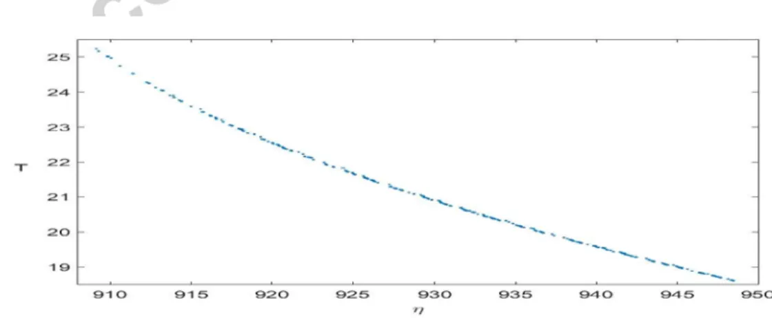
For each blend, the viscosity is instrumentally determined, and the clear point refers to the temperature at which the detergent appears cloudy again after prior heating at 80 ºC. The final goal is to determine the mixture that improves the effectiveness of the hydrotrope, that is, minimum values for both T and η.
In this case, there are four factors in the blend, so the simplex mixture space is already in three dimensions, which makes it more difficult the interpretation of the models fitted. Further, with two experimental responses to be simultaneously minimized, we need to study the possible trade-off solutions and the effect of the factors on the different responses, when only considering optimal solutions.
Finally, another characteristic of the problem is that the experimental domain has additional constrains, further to the usual total amount of component proportions equal to one, eq. (1). These restrictions impose that the relative quantity of STS vary in [0.10, 0.60], SXS must be in [0.10, 0.50], Na2SO4 in [0.05, 0.40], and the proportion of SBS varies in [0.05, 0.30].
In this constrained domain, we estimate the pareto-optimal front by using the models fitted to T and η, which adequately described the experimental results obtained with a D-optimal design with 32 experiments. There are four factors to be mixed so the quadratic model has the same ‘crossproducts model’ expression of equation (2). The details of the fitting and validation of the models, as well as the selection of the experimental design in this constrained experimental domain, can be consulted in the cited paper [21].
With the general ideas of the procedure explained in [15], the algorithm is adapted to work in mixture experimental designs additionally taking into account the constraints in the domain. For the case at hand, to estimate the front, a population of 500 mixtures in the constrained four-dimensional experimental domain evolves during 5000 generations with probability of mutation equal to 0.2. The final population is made up by 487 non-dominated solutions, i.e., mixtures that provide viscosity or temperature of the resulting detergent with the property of being the minimum possible value in at least one of them. These mixtures in the front provide values of viscosity, η, from 908.90 to 948.47 whereas T (the clear point) is expected to achieve values in the experimental domain from 18.61 ºC to 25.29 ºC.
Page 9/ 19 point versus viscosity) that shows the conflict between the responses, the pareto-optimal front shows the typical curvature directed towards the origin, which is clearly interpreted: the decreasing of one of the coordinates necessarily requires the increase of the value in the other coordinate. In other words, going down in the front (better clear point) requires necessarily moving to the right (worse viscosity) or equivalently, to move to the left to improve viscosity is possible provided you go up along the front, worsening the achievable clear point.
Figure 1
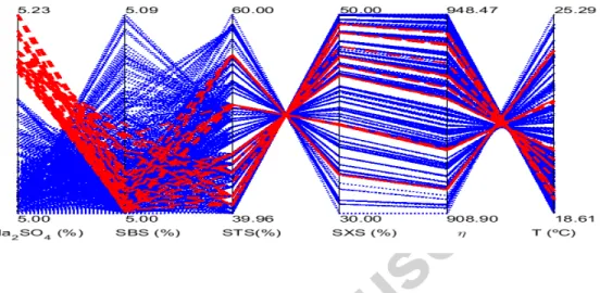
An alternative representation of the solutions found, in the form of a parallel coordinates plot with some adaptation [6] to improve visualization, is in figure 2. As can be seen, this plot is not limited in the number of coordinates to be represented and, for the problem at hand, allows representing together the mixtures of the four compounds and the two responses.
Figure 2
In figure 2, the first four coordinates are for the percentages of Na2SO4, SBS, STS and SXS,
respectively; the remaining two coordinates are for the expected values of viscosity and clear point, respectively. Each broken line joining mixtures to responses represents one of the pareto-optimal solutions found. Finally, as the scales are modified to improve visualization, the numbers up and down each coordinate are the minimum and maximum values, respectively, for the corresponding coordinate.
In this way, the same values seen in fig. 1 can also be seen in the last two coordinates in figure 2. The minimum values among the results of the experimental design were for η = 900, and T = 19 ºC and they are achieved (taking into account the variability of the determinations) in the solutions in the pareto-optimal front. On the other hand, the largest values obtained among the experiments carried out of η = 1900 and T = 73 ºC are substantially reduced for the pareto-optimal mixtures.
Like in figure 1, when looking at the mentioned last two coordinates of figure 2, the conflicting behaviour of the two objectives is also apparent: the lines coming from the coordinate for η to the one for T cross each other like maintaining a fixed point in between. That clearly implies that low values of η (in the range described by the optimal solutions) correspond to large values of T and vice versa. In other words, to decrease the viscosity η an increase in T should be assumed and vice versa. Also, the region for the lowest value of T seems to be much more populated than the one corresponding to the minimum values of viscosity, which suggests that by mixing the four compounds within the specified ranges it is more difficult to reduce the viscosity than the temperature of clear point.
Regarding the mixtures to achieve these values of the responses, they are depicted in the first four coordinates of figure 2. The limits in each coordinate are written in percentage to better perceive the slight differences among solutions, as far as the first two coordinates is concerned, that is, the contribution of sodium sulfate Na2SO4 and sodium benzenesulfonates,
Page 10/ 19 The first conclusion is that, in practice, the variation in the values in figure 2 are obtained with mixtures of only two of the components, STS and SXS, third and fourth coordinates, because all the solutions in the pareto-optimal front share the fact that SBS and Na2SO4 are,
in practice, constant at their minimum achievable value, 5 %. The only characteristic that might be mentioned is that a slight increase of Na2SO4 (more than 5.15 %, up to 5.23 %)
observable in the red dashed lines in figure 2 causes the loss of the minimum allowable values in both responses, especially for viscosity. Other than that, it is also patent that with 5% of both Na2SO4 and SBS, the remaining coordinates still cover all the values seen in
figure 2, in particular, all the expected allowable values of both responses.
The pattern of crossing lines with a fixed point in between already mentioned for the coordinates corresponding to the experimental responses is also observed in the coordinates corresponding to STS, the third, and SXS, the fourth.
Despite the explanation just exposed about the interpretation of this graphical behaviour as an opposed behaviour (pointing to conflict among responses or opposed effect of the factors on the responses), we should keep in mind that for mixture designs, the total amount is constant so this is exactly what we were expecting in the factors of the mixture. Of course, the lines that crisscross only between the third and fourth coordinates shows the opposed behavior only there because both the sodium sulfate and SBS are almost kept constant at 5%.
Furthermore, increasing proportions of STS, from 40 % to 60 % of the blend, linked to decreasing proportions of SXS, from 50 % to 30 %, provide better (lower) values of viscosity, although larger temperatures of clear point, T. On the contrary, given the opposite behaviour, if the best values of T are sought, the quantity of SXS should be increased, and STS accordingly decreased.
Notice that these decisions about how to modify the proportions of STS and SXS are related to the lowest possible value in one of the responses for a given value of the other. The fact that SBS and Na2SO4 in the mixture should be set at 5% says that the two responses are very
sensitive to these factors when it is about minimizing both of them. Consequently, and given that 5% is the lowest proportion allowed, the increasing of any of them causes that the corresponding mixture is no longer optimal, i.e. it necessarily worsens the expected experimental responses, although it is difficult to quantify how much.
3.2.Optimization of an admixture for concrete
Page 11/ 19 In this case, the simplex mixture space is four-dimensional (five admixture components to be mixed) and constrained because D and E have both an upper bound, 18 % and 5%, respectively. In this experimental domain, four experimental models are fitted and analysed for water reduction (%) and for the compressive strengths (Mpa) on mortar after 1, 7, and 28 days. Experimental conditions (proportions of the components in the mixture) are sought for maximal strength and loss of water.
The results obtained in the cited paper [22] are separately discussed per dosage level, so three different models are handled for each response. In the present work, although the dosage level can be a continuous factor, we interpret it in terms of ‘blocking’. Blocking can be used to transform into factors of the design those variables that are known or suspected of experiencing discrete changes throughout the experiment or that, in general, are difficult to control but only have, if any, an additive effect.
In the original work, authors maintain the dosage level constant among some experiments and then changed it, but it was kept constant in a different group of experiments, so that the possible effect of different dosage level can be modelled as if the experiments were conducted in blocks.
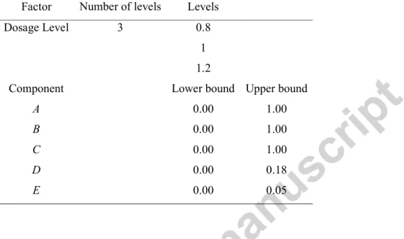
Consequently, we set up the corresponding blocked design and re-interpret the whole experimental results by considering them all together in the definition of a blocked mixture design. Table 1 summarizes the experimental domain when considering the new experimental design, where the dosage level is used as a discrete variable with three levels and the remaining five chemical components of the admixture are continuous, though linearly dependent, variables that further vary in a constrained domain.
Table 1.
The variance function with this design remains below 0.46 in the whole experimental domain, so the design is adequate because the main goal of the fitted models is to predict values of the responses in the experimental domain.
Only binary synergisms were modelled by means of a full quadratic model with 17
Notice that there are two terms in eq. (5) linked to the ‘block’ factor, namely the dosage level. Because there are three blocks, the two coefficients β1A and β1B are multiplying two variables
that are in fact indicator (binary) variables, in this case, X1A = 1 when the dosage level used
was 0.8% and 0 otherwise, whereas X1B = 1 when dosage level is 1.0% and 0 otherwise. That
Page 12/ 19 The coefficients estimated for the four response variables being handled are in table 2 together with some usual statistics. Regarding the validation of the fitted models, no outlier residual or lack of normality have been found in any of the models. The significance test refers to the hypothesis test whose null hypothesis is that all the coefficients are null as against the alternative hypothesis that at least one of them is non-null. The p-values of the significance tests in table 2 (penultimate row) lead to conclude that the four models are statistically significant, at 5% significance level. They describe 89.9 %, 90.1 %, 79.4 % and 83.6 % of the variance of the corresponding response, according to R2 for water reduction
(WR), compressive strength after 1 day (S1), after 7 days (S7) and after 28 days (S28), respectively.
Table 2.
There are a total of four experiments (one for 0.8 % and 1.2 % and two for 1.0 % dosage levels) replicated twice, so that an estimation of the pure error can be obtained to test for lack of fit, LOF. The null hypothesis in this case is that there is not bias, as against a biased model. With the p-values associated with the decision in the last row of table 2, there is no evidence of LOF in the models, except for the significant bias detected in the model of S1, at 5% significance level, despite being the model with the largest coefficient of determination, R2. A
similar behaviour is observed in some of the models for S1 in [22] that the authors attribute to the fact that, for this response, the replicates are very similar (when not exactly the same) so that the pure error is estimated as practically null, leading to a significant lack of fit. Thus, with some reservations, the model is accepted.
Regarding the block effect, the estimated coefficients b1A are statistically non-null (5%
significance level) for all the responses, except for S7. Taking into account the sign, one can say that using 0.8 % dosage level significantly decreases WR; and the compressive strength can be improved (larger values are desired for the compressive strength no matter the elapsed time) at the beginning (after 1 day) but finally, after 28 days, gets significantly worse. Using 1.0 % of dosage level, b1B, does not have effect on the responses, except may be for S1. This
also points out a possible conflicting behaviour between S1, S7 and S28 that was not necessarily expected. And the relation between strengths and water reduction is not clear either.
In any case, the joint optimization (maximum values for all the responses) requires the study of the possibly conflicting behaviour, and to look for trade-off solutions. Again, this study is made by searching the pareto-optimal front for the four experimental responses depending on the five factors (the chemical components) but also the discrete factor that models the dosage level should be taken into account. To do this, after the usual crossover and mutation in the mixture space of the five components, the corresponding off-springs are used with all the dosage levels and enter to the selection phase based on non-dominance.
With a population of 200 mixtures with different dosage level and with D less than 18 % and
Page 13/ 19 compressive strength after one day that gets at most 64.22 Mpa after seven days and 71.69 Mpa after 28 days, though not for the same admixture.
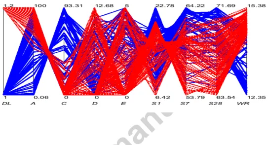
This can be seen in figure 3 that depicts the pareto-optimal front in the form of a parallel coordinates plot. It is clear the advantage of using parallel coordinates plot to represent together the five factors (A-E) plus the dosage level (DL) plus the four experimental responses, compressive strengths (after 1, 7 and 28 days) and water reduction (WR). Not surprisingly given the interpretation of the coefficients related to the block in the fitted models, the admixtures are mostly, but not exclusively, for dosage level of 1 % and 1.2 % and, remarkably, all of them with the property of having the proportion of B equal to 0 %, i.e. no B component in the admixture.
Figure 3
In particular, dashed red lines superimposed in figure 3 highlight the only six solutions found optimal when the dosage level is 0.8 %, clearly linked to the best possible value for the strength after one day, S1, and the worst values for the remaining three responses. Further to the 0.8 % of dosage level, and B = 0 %, these admixtures share the fact that also D = E = 0 % thus the admixture is made exclusively with A and C, with larger proportion of component A. Although with the rescaling to improve visualization the original scales are not evident in figure 3, to achieve the best strength after one day, as predicted by the fitted model, component A should be between 61.4 % to 83.6 % of the total admixture with the corresponding proportion of C decreasing from 38.6 % to 16.4 % for achieving compressive strengths after 7 days, S7, less than 52.3 Mpa, that remain below 62.8 Mpa after 28 days, S28, and water reduction WR at most of 12.3 %.
More populated is the pareto-optimal front for solutions with dosage level 1 % and 1.2 %, blue dotted lines in figure 3, that cover almost the whole range allowable for component A, and E (bounded from above by 5%), no more than 93.3 % of C and up to almost 13 % of the limiting 18 % allowed for component D.
By removing from the graph the coordinate for B, which is constant, and the solutions corresponding to 0.8 % of dosage level, the new parallel coordinates plot, rescaled with the corresponding extreme values, is in figure 4, pointed blue lines for dosage level of 1 %, dashed red lines for 1.2 %. The new limits seen in figure 4 show that with the mixtures detailed in the previous paragraph, the expected values of the compressive strengths are maintained larger than 6.42 Mpa after one day, 53.79 Mpa after 7 days and 63.54 Mpa after 28 days, and the remaining response, water reduction is always above 12.3 %.
Figure 4
Page 14/ 19 in this range of C and 1.2 % dosage level, the increase of A (which should be no less than 55 %) mostly linked to reduction of D and E causes the increase of water reduction with decreasing values of the three values of strength.
figure 5
4. CONCLUSIONS
The adaptation and implementation of a tool to compute the pareto-optimal front in multi-response mixture designs, joint to the use of graphs in the form of parallel coordinates plot, allow handling and more easily interpreting experimental results via the fitted model, and also finding optimal experimental conditions that provide a compromising solution among several conflicting responses.
The procedure is also extended to cover some increasingly need of ‘ad-hoc’ experimental design, showing that it can be useful with ‘combined’ nonclassical designs that contain, in the case shown, continuous mixture proportions and discrete levels of some factors, which may be the result of a block design. This opens a route for the use of these tools in problems with process variables and mixtures.
ACKNOWLEDGEMENT
The authors acknowledge the financial support of Spanish Ministerio de Economía y Competitividad through project CTQ2014-53157-R, a national competitive project co-financed with European FEDER funds.
FIGURE CAPTIONS
Page 15/ 19 Figure 2. Parallel coordinates plot of the pareto-optimal front estimated for case in section
3.1. Percentages of SBS for sodium benzenesulfonates, STS is for sodium toluenesulfonates, SXS for sodium xylenesulfionates. η is the viscosity and T is the clear point. Different line types and colour separate the solutions with more (dashed red lines) or less (dotted blue lines) than 5.15 % of sodium sulphate.
Figure 3. Parallel coordinates plot of the pareto-optimal front for the optimization of concrete in section 3.2. DL is the dosage level, A-E are for the proportions of the corresponding chemicals (%); S1 (Mpa) is the compressive strength after one day,
Page 16/ 19 Figure 4. Parallel coordinates plot of the pareto-optimal solutions in section 3.2 only for
dosage level 1 % (blue continuous lines) or 1.2 % (dotted red lines), and removing the coordinate for B (which is always 0%). DL is the dosage level, A-E are for the percentage of these chemicals; S1 (Mpa) is the strength after one day, S7 (Mpa) after 7 days, and S28 (Mpa) after 28 days, WR (%) is water reduction.
Page 17/ 19
Tables
Table 1. Experimental domain for the blocked mixture design of case in section 3.2
Factor Number of levels Levels
Dosage Level 3 0.8
1 1.2
Component Lower bound Upper bound
A 0.00 1.00
B 0.00 1.00
C 0.00 1.00
D 0.00 0.18
E 0.00 0.05
Table 2. Estimated coefficients (bi), standard error of estimation, sy/x, and determination coefficient R2 of the models fitted for water reduction (WR), and compressive strength after one (S1), seven (S7) and 28 (S28) days. Also, p-values for both significance and lack of fit (LOF) tests
WR S1 S7 S28
b1A -2.099* 2.689* -1.691 -2.063*
b1B -0.641 2.648* 1.034 0.825
b2 14.511 19.972 54.539 63.539
b3 6.33 15.587 42.15 54.144
b4 11.72 18.607 54.456 63.704
b5 -9.586 -215.02 -251.74 -218.39
b6 161.54 875.45 -3784.4 -261.8
b23 2.12 -4.018 5.286 4.105
b24 2.389 3.072 -3.641 5.449
b25 34.274 186.88 406.82 374.66
Page 18/ 19
b34 -3.918 -5.71 -5.6 -4.289
b35 38.376 213.05 464.88 422.65
b36 -149.23 -951.62 4178.1 459.86
b45 32.295 192.2 407.67 367.75
b46 -119.46 -953.32 4161.7 416.64
b56 -204.06 -1159.4 3434.3 98.506
sy/x 1.163 0.643 2.998 2.094
R2
0.899 0.901 0.794 0.836
p-value
(signif.test) < 10-4 < 10-4 < 10-4 < 10-4
p-value
(LOF) 0.603 0.0039 0.942 0.372
* Indicates a significant block effect (the coefficient is significantly non-null at 5% significance level)
REFERENCES
[1] W.L. Smith, Experimental design for formulation, ASA-SIAM series on Statistics and Applied Probability, SIAM, Philadelphia, ASA, Alexandria, VA, 2005.
[2] C. Reguera, M.S. Sánchez, M.C. Ortiz, L.A. Sarabia, Pareto-optimal front as a tool to study the behaviour of experimental factors in multi-response analytical procedures, Anal. Chim. Acta 624 (2008) 210.
[3] M.S. Sánchez, M.C. Ortiz, L.A. Sarabia, Selection of nearly orthogonal blocks in ‘ad-hoc’ experimental designs, Chemom and Intell Lab Systems 133 (2014) 109.
[4] M.S. Sánchez, L.A. Sarabia, M.C. Ortiz, On the construction of experimental designs for a given task by jointly optimizing several quality criteria: Pareto-optimal experimental designs, Anal. Chim. Acta 754 (2012) 39.
[5] A. Herrero, C. Reguera, M.C. Ortiz, L.A. Sarabia, M.S. Sánchez, Ad-hoc blocked design for the robustness study in the determination of dichlobenil and 2,6-dichlorobenzamide in onions by programmed temperature vaporization-gas chromatography-mass spectrometry, Journal of Chromatography A 1370 (2014) 187. [6] M.C. Ortiz, L.A. Sarabia, M.S. Sánchez, D. Arroyo, Improving the visualization of the
Pareto-optimal front for the multi-response optimization of chromatographic determinations, Anal. Chim. Acta 687 (2011) 129.
[7] M.S. Sánchez, M.C. Ortiz, L.A. Sarabia, R. Lletí, On Pareto-optimal fronts for deciding about sensitivity and specificity in class-modelling problems, Anal. Chim. Acta 544 (2005) 236.
Page 19/ 19 [9] D. Voinovich, B. Campisi, and R. Phan-Tan-Luu, Experimental Design for Mixture
Studies.In: Brown S, Tauler R, Walczak R (eds.) Comprehensive Chemometrics, volume 1, Elsevier, Oxford, 2009, pp. 453-498.
[10] J.A. Cornell, Mixture experiments. In: Statistical design and analysis of industrial experiments, edited by Subir Ghosh, Marcel Dekker, Inc., New York, 1990, pp. 175-209.
[11] J.A. Cornell, Experiments with Mixtures: Designs, Models, and the Analysis of Mixture Data, 3rd ed., John Wiley & Sons, New York, 2002.
[12] R. Phan-Tan-Luu, M. Sergent, Nonclassical Experimental Designs. In: Brown S, Tauler
R, Walczak R (eds.) Comprehensive Chemometrics, volume 1, Elsevier, Oxford, 2009, pp. 391-452.
[13] L.A. Sarabia and M.C. Ortiz, Response Surface Methodology. In: Brown S, Tauler R, Walczak R (eds.) Comprehensive Chemometrics, volume 1, Elsevier, Oxford, 2009, pp. 345-390.
[14] L.A. Sarabia, M.S. Sánchez, M.C. Ortiz, Introduction to ranking methods In: Manuela Pavan and Roberto Todeschini, editors, Scientific Data Ranking Methods: Theory and Applications, Data Handling in Science and Technology, Elsevier, 2008, pp. 1-50. [15] M.C. Ortiz, L.A. Sarabia, A.Herrero, M.S. Sánchez, Vectorial optimization as an
alternative to desirability functions, Chemom and Intell Lab Systems 83 (2006) 157. [16] K. Deb, Multiobjective Optimization using Evolutionary Algorithms, Wiley,
Chichester, 2001.
[17] A. Inselberg, Parallel Coordinates: Visual Multidimensional Geometry and Its Applications, Springer, 2009.
[18] R. Cela, M.H. Bollaín, New cluster mapping tools for the graphical assessment of non-dominated solutions in multi-objective optimization, Chemom and Intell Lab Systems 114 (2012) 72.
[19] T. Tušar, and B. Filipicˇ, Visualization of pareto front approximations in evolutionary multiobjective optimization: a critical review and the prosection method, IEEE transactions on evolutionary computation 19 (2015) 225.
[20] A. Ibrahim, S. Rahnamayan, M. Vargas, K. Deb, 3D-RadVis: Visualization of Pareto Front in Many-Objective Optimization, COIN Report Number 2016013. Collected on September 2, 2016, in www.egr.msu.edu/~kdeb/papers/c2016013.pdf
[21] A. Kamoun, M. Chaabouni, M. Sergent, R. Phan-Tan-Luu, Mixture design applied to the formulation of hydrotropes for liquid detergents, Chemom and Intell Lab Systems 63 (2002) 69.