LOW X RAY LUMINOSITY GALAXY CLUSTERS: MAIN GOALS, SAMPLE SELECTION, PHOTOMETRIC AND SPECTROSCOPIC OBSERVATIONS

LOW X-RAY LUMINOSITY GALAXY CLUSTERS: MAIN GOALS, SAMPLE SELECTION,

PHOTOMETRIC AND SPECTROSCOPIC OBSERVATIONS

José Luis Nilo CastellÓn1,2, M. Victoria Alonso3,4, Diego García Lambas3,4, Carlos Valotto3,4, Ana Laura O’Mill3,4, Héctor Cuevas1, Eleazar R. Carrasco5, Amelia Ramírez1, José M. Astudillo6, Felipe Ramos3,

Marcelo Jaque Arancibia7, Natalie Ulloa1, and Yasna Órdenes8

1

Departamento de Física y Astronomía, Facultad de Ciencias, Universidad de La Serena, Cisternas 1200, La Serena, Chile

2

Dirección de Investigación, Universidad de La Serena. Av. R. Bitrán Nachary 1305, La Serena, Chile

3_{Instituto de Astronomía Teórica y Experimental,(IATE-CONICET), Laprida 922, Córdoba, Argentina} 4

Observatorio Astronómico de Córdoba, Universidad Nacional de Córdoba, Laprida 854, Córdoba, Argentina

5

Gemini Observatory/AURA, Southern Operations Center, Casilla 603, La Serena, Chile

6

Departamento de Ciencias Físicas, Universidad Andrés Bello, Av. República 252, 837-0134 Santiago, Chile

7

Instituto de Ciencias Astronómicas, de la Tierra y del Espacio(ICATE-CONICET), Av. España Sur 1512, J5402DSP, San Juan, Argentina

8

Argelander Institute für Astronomie der Universität Bonn, Auf dem Hügel 71, D-53121 Bonn, Germany Received 2015 December 1; accepted 2016 March 22; published 2016 May 25

ABSTRACT

We present our study of 19 low X-ray luminosity galaxy clusters(LX~0.5–45×1043erg s−1), selected from the ROSAT Position Sensitive Proportional Counters Pointed Observations and the revised version of Mullis et al. in the redshift range of 0.16–0.7. This is the introductory paper of a series presenting the sample selection, photometric and spectroscopic observations, and data reduction. Photometric data in different passbands were taken for eight galaxy clusters at Las Campanas Observatory; three clusters at Cerro Tololo Interamerican Observatory; and eight clusters at the Gemini Observatory. Spectroscopic data were collected for only four galaxy clusters using Gemini telescopes. Using the photometry, the galaxies were defined based on the star-galaxy separation taking into account photometric parameters. For each galaxy cluster, the catalogs contain the point-spread function and aperture magnitudes of galaxies within the 90% completeness limit. They are used together with structural parameters to study the galaxy morphology and to estimate photometric redshifts. With the spectroscopy, the derived galaxy velocity dispersion of our clusters ranged from 507 km s−1for[VMF98]022 to 775 km s−1for[VMF98]097 with signs of substructure. Cluster membership has been extensively discussed taking into account spectroscopic and photometric redshift estimates. In this sense, members are the galaxies within a projected radius of 0.75 Mpc from the X-ray emission peak and with clustercentric velocities smaller than the cluster velocity dispersion or 6000 km s−1, respectively. These results will be used in forthcoming papers to study, among the main topics, the red cluster sequence, blue cloud and green populations, the galaxy luminosity function, and cluster dynamics.

Key words:galaxies: clusters: general– galaxies: fundamental parameters–galaxies: photometry

1. INTRODUCTION

The hierarchical model of structure formation predicts that the progenitors of the galaxy clusters are relatively small systems that are assembled together at higher redshifts. Local cluster processes such as ram pressure stripping and galaxy harassment play an important role in explaining the difference between cluster and field galaxy populations at afixed stellar mass (Berrier et al. 2009). The study of galaxy systems in a variety of masses at different redshifts may give invaluable physical insights into galaxy evolution.

The observed galaxy scaling relationships provide important tools for examining physical properties of galaxies and their systematics. These relations might be linked to the local galaxy density in rich clusters (e.g., Dressler 1980) or the galaxy morphology evolution(e.g., Butcher & Oemler1984; Dressler & Gunn 1992). Their connection with different mechanisms such as galaxy collisions (Spitzer & Baade 1951) and interactions with intracluster gas (Gunn & Gott 1972) are crucial to understand galaxy formation and evolution. When a galaxy cluster is assembled, the morphology, luminosity, mass, and mean stellar age of their member galaxies are determined by these processes.

Kodama et al.(1998)studied the Color–Magnitude Relation (CMR)in distant clusters and suggested the monolithic model

for the formation of early-type galaxies, but also mentioned other possibilities. In particular, an alternative scenario is the hierarchical merging model(Kauffmann & Charlot 1998; De Lucia et al. 2004). The red cluster sequence found in optical CMRs (hereafter RCS; Gladders et al. 1998; De Lucia et al. 2004; Gilbank et al.2008; Lerchster et al.2011hereafter RCS), which is dominated by non-star-forming, early-type galaxies (Blanton & Moustakas2009; Zhu et al.2010)can be used to test these models. Changes in the slope and zero-point of this relation may be an indication of cluster evolution. In the CMRs, star-forming, late-type galaxies populate the “blue cloud.”The presence of these two populations emerges as a bimodality in the color distribution(Baldry et al.2004)as well as a“green valley”between them (see, for instance, Mendez et al.2011). The combination of deep images with multi-object spectrographs makes it possible to explore additional evidence related to the processes responsible for the observed properties of cluster members (Christlein & Zabludoff 2005) and to understand better their relationships with the environment (Finn et al.2005).

and interactions as a function of redshift and environments, are among the main issues addressed by these surveys. We can mention: the ESO Distant Cluster Survey(EDisCS, White et al. 2005) in a wide range of mass, with redshifts from 0.4 to almost 1.0; the X-ray-luminous clusters from the MACS survey at z ≈0.5 within a 1.2 Mpc diameter (Stott et al.2007); the Observations of Redshift Evolution in Large-Scale Environ-ments (ORELSE) Survey (Lubin et al. 2009), a systematic search for structure around well-known clusters at redshifts of 0.6<z<1.3; the galaxy populations in the core of a massive, X-ray luminous cluster(Strazzullo et al.2010)atz=1.39; and the IMACS Cluster Building Survey (Oemler et al. 2013)to understand the large-scale environment surrounding rich intermediate redshift clusters of galaxies.

On the other hand, regarding less massive clusters, Balogh et al. (2002) presented the first spectroscopic survey of low X-ray luminosity clusters (LX <4 ´1043h−2erg s−1 [0.1–2.4]keV)with Calar Alto spectroscopy andHubble Space Telescope WFPC2 imaging at 0.23<z<0.3. These clusters have Gaussian velocity distributions, with velocity dispersions (σ)ranging from 350 to 850 kms−1, consistent with the local LX–σrelation. The spectral and morphological properties of the galaxies in these systems were found similar to those in massive clusters at the same redshifts. Carrasco et al. (2007) analyzed the properties of the low luminosity X-ray cluster of galaxies RX J1117.4+0743 atz=0.485 based on optical and X-ray datafinding a complex morphology composed of at least two structures in velocity space. This cluster also presents an offset between the Bright Group Galaxy and the X-ray emission. More recently, Connelly et al. (2012) have investigated systems detected in both X-rays and the optical in the redshift range 0.12 < z < 0.79, obtaining an LX–σ scaling relation similar to observed in nearby groups.

The X-ray properties of groups in 0.2<z<0.6 are the same as those observed at lower redshifts (Jeltema et al. 2006; Mulchaey et al. 2006). In some cases, it was found that the X-ray emission was clearly peaked in the most luminous early-type galaxy. There is also evidence that the central galaxy is composed of multiple luminous nuclei, suggesting that the brightest galaxy may still be undergoing major mergers. At higher redshifts(0.85<z<1), Balogh et al.(2011)studied the morphology of galaxies in six galaxy groups,finding that they are dominated by red galaxies like lower-redshift groups. A few galaxies populate the“blue cloud”and there is a significant number of galaxies with intermediate colors, which are a probable transient population.

Within this context, we aim at contributing to galaxy formation and evolution by analyzing a sample of low X-ray luminosity galaxy clusters at intermediate redshifts. Our analysis can shed light on the properties of these systems, in particular, the role of interactions in the formation of galaxy clusters. In this paper, we describe the cluster sample and the data comprising photometric observations obtained at Las Campanas Observatory(LCO)and Cerro Tololo Interamerican Observatory (CTIO), and photometric and spectroscopic data obtained at the Gemini Observatory. These data will be used to study different galaxy populations in the clusters, as well as the galaxy luminosity function and cluster dynamics. We have already published Nilo Castellón et al. (2014) and Gonzalez et al.(2015)on photometric galaxy properties and weak lensing analysis, respectively, using part of this data set. The sample of low X-ray galaxy clusters is defined in detail in Section2, the

photometric observations and the reduction procedures are given in Section3including source detections and photometry, magnitude calibration, limiting magnitudes, and completeness. In Section 4, the spectroscopic observations and data reduc-tions are presented. In Section 5, the cluster membership assignment procedure is addressed together with an outline of the photometric redshift estimates. Finally, in Section 6, we present a brief comments on the project, the main results already obtained and future plans. For all cosmology-dependent calculations, we have assumed WL = 0.7,

Wm=0.3, andh=0.7.

2. LOW X-RAY LUMINOSITY CLUSTER SAMPLE

Vikhlinin et al.(1998)presented the catalog of 223 galaxy clusters based on the spatial extent of their X-ray emission, serendipitously detected in the ROSAT Position Sensitive Proportional Counters (PSPC) pointed observations with photometric redshift estimates. This catalog of extended X-ray sources was revised by Mullis et al.(2003)using optical imaging and spectroscopy to classify 200 galaxy clusters, excluding 23 false detections. The spectroscopic cluster redshifts were derived by long-slit and multiobject spectra with at least 2 or 3 concordant galaxy redshifts per cluster, always including the Bright Cluster Galaxy (BCG), and they entirely superseded the photometric estimates of Vikhlinin et al.(1998).

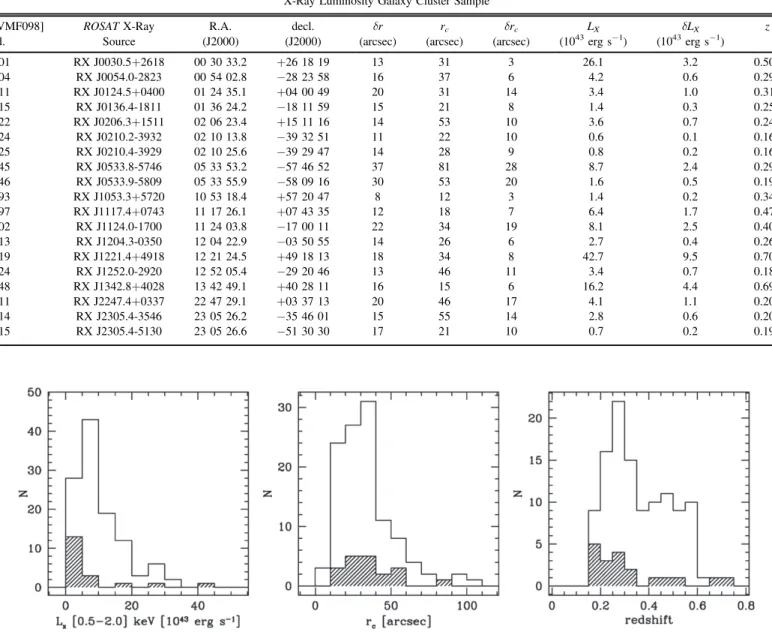
For the present work, we have selected systems with X-ray luminosities in the [0.5–2.0]keV energy band (rest frame), which is close to the detection limit of theROSATPSPC survey ranging from 0.1 to 50´1043_{erg s}−1_{. These luminosities could} be affected by the presence of not removed point sources such as AGNs from the X-ray emission. This effect could be more important at lower luminosities, for instance groups containing an AGN could be wrongly included in the sample. The redshift range of our selection is 0.16–0.70 where we have excluded well-studied low-redshift clusters as well as the galaxy cluster [VMF98]061 at z > 1 previously analyzed by Rosati et al. (1999). Within these luminosity and redshift limits, we have a sample of 140 galaxy clusters with low X-ray luminosities. After visual inspection, we have avoided those fields with bright stars and also those extended objects that would require more than one image to cover the field with the available instruments and telescopes. In this way, our studied sample corresponds to a random selection of 19 low X-ray galaxy clusters. Table1presents a summary of the main characteristics of this studied galaxy cluster sample. Columns(1)and(2)show the Vikhlinin et al. (1998) and the ROSAT X-ray survey identifications. The equatorial coordinates of the X-ray centroid and the position uncertainties are in columns (3)–(5); the cluster angular core radius (in arcsec) and the corresponding error are given in columns(6)and(7); the X-ray luminosity in the [0.5–2.0]keV energy band and estimates of the lower bound of their uncertainties are in columns(8)and(9); and the mean redshift in column(10). Columns(3)–(7)are taken from Vikhlinin et al. (1998) while columns (8) and (10) are from Mullis et al. (2003). The mean X-ray luminosity is 7.3×1043erg s−1, an intermediate/low luminosity when compared to ~1042_{erg s}−1 _{for groups with extended X-ray} emission or larger values than ~ ´5 1044_{erg s}−1

of rich clusters.

histograms)compared to the 140 galaxy clusters selected from Mullis et al.(2003). It can be appreciated that our sample of 19 galaxy clusters is biased toward low X-ray luminosities and lower redshifts since we aim at studying this particular regime. The mean angular core radius was about 35 arcsec and most of the galaxy clusters had values smaller than 60 arcsec.

Figure 2 shows the cluster X-ray luminosities (L500 [0.1–2.4]keV) versus redshifts of our galaxy cluster sample and the total sample from Mullis et al.(2003)represented with different circles. We also include other works: Girardi & Mezzetti (2001), Popesso et al. (2005), Wake et al. (2005), and Jensen & Pimbblet (2012). These studies analyze the cluster membership and the photometric properties as galaxy colors and CMRs as our study. All the X-ray luminosities are in the same system, extracted from Piffaretti et al. (2011) which is the largest X-ray galaxy cluster compilation based on publicly availableROSATAll Sky Survey data. In the redshift range studied here, we have chosen the galaxy clusters with

lower X-ray luminosities after discarding those mentioned above.

The main goal of this work is to provide keys to understand the cluster assembly and the morphological evolution of galaxies in low X-ray luminosity clusters. These systems thus provide us an interesting environment to explore the efficiency of mergers and ram pressure effects, that can be significantly different from those of rich galaxy clusters. Our study is based on photometric observations of these low X-ray luminosity systems, where the high-quality images also allowed us to construct a morphological catalog to study galaxy morpholo-gies and scaling relations. We are particularly interested in a detailed study of the RCS and an analysis of an eventual intermediate green galaxy population between the galaxy blue cloud and the RCS in these low X-ray systems(Mendez et al. 2011). For some galaxy clusters, we also carried out spectro-scopic observations which allowed us to determine cluster membership and velocity dispersion estimates.

Table 1

X-Ray Luminosity Galaxy Cluster Sample

[VMF098] ROSATX-Ray R.A. decl. δr rc δrc LX δLX z

Id. Source (J2000) (J2000) (arcsec) (arcsec) (arcsec) (1043erg s−1) (1043erg s−1)

001 RX J0030.5+2618 00 30 33.2 +26 18 19 13 31 3 26.1 3.2 0.500

004 RX J0054.0-2823 00 54 02.8 −28 23 58 16 37 6 4.2 0.6 0.292

011 RX J0124.5+0400 01 24 35.1 +04 00 49 20 31 14 3.4 1.0 0.316

015 RX J0136.4-1811 01 36 24.2 −18 11 59 15 21 8 1.4 0.3 0.251

022 RX J0206.3+1511 02 06 23.4 +15 11 16 14 53 10 3.6 0.7 0.248

024 RX J0210.2-3932 02 10 13.8 −39 32 51 11 22 10 0.6 0.1 0.168

025 RX J0210.4-3929 02 10 25.6 −39 29 47 14 28 9 0.8 0.2 0.165

045 RX J0533.8-5746 05 33 53.2 −57 46 52 37 81 28 8.7 2.4 0.297

046 RX J0533.9-5809 05 33 55.9 −58 09 16 30 53 20 1.6 0.5 0.198

093 RX J1053.3+5720 10 53 18.4 +57 20 47 8 12 3 1.4 0.2 0.340

097 RX J1117.4+0743 11 17 26.1 +07 43 35 12 18 7 6.4 1.7 0.477

102 RX J1124.0-1700 11 24 03.8 −17 00 11 22 34 19 8.1 2.5 0.407

113 RX J1204.3-0350 12 04 22.9 −03 50 55 14 26 6 2.7 0.4 0.261

119 RX J1221.4+4918 12 21 24.5 +49 18 13 18 34 8 42.7 9.5 0.700

124 RX J1252.0-2920 12 52 05.4 −29 20 46 13 46 11 3.4 0.7 0.188

148 RX J1342.8+4028 13 42 49.1 +40 28 11 16 15 6 16.2 4.4 0.699

211 RX J2247.4+0337 22 47 29.1 +03 37 13 20 46 17 4.1 1.1 0.200

214 RX J2305.4-3546 23 05 26.2 −35 46 01 15 55 14 2.8 0.6 0.201

215 RX J2305.4-5130 23 05 26.6 −51 30 30 17 21 10 0.7 0.2 0.194

3. PHOTOMETRY

In this section, we show the observations and the photo-metric procedures adopted to obtain the galaxy properties of our cluster sample.

3.1. Observations

The galaxy clusters selected for this study have been observed using LCO, CTIO, and Gemini Observatory.

Eight galaxy clusters at z < 0.32 were observed at LCO using the 2.5 m du Pont telescope with the Wide Field Reimaging CCD Camera (TEK#5 CCD) for direct imaging with a scale of 0.77 arcsec/pixel over afield of 25 arcminute diameter using Chilean time allocation. The images were obtained in theB V R, , ,andIJohnson–Cousinsfilters in nights with variable atmospheric conditions. The seeing values were less than 1 arcsec in two galaxy clusters and between 1.2 and 1.8 arcsecs in the remaining systems. Six galaxy clusters were observed in the four passbands while the clusters[VMF98]011 and[VMF98]211 were observed only in theBandRpassbands due to poor atmospheric conditions.

Three galaxy clusters at 0.19<z<0.30 were observed at CTIO using the Victor Blanco 4 m telescope and the MOSAIC-II camera, which is an array of eight 2048×4096 SITe CCDs, with a scale of 0.27 arcsec/pixel, giving a total field of view (FOV) of 36×36 arcmin. The images were taken in the

B V R, , ,andIJohnson–Cousins passbands using the Director

Discretionary Time. The median seeing of the observations were about 0.85 arcsec.

Finally, eight galaxy clusters with 0.18 < z < 0.70 were obtained using the 8 m Gemini north (GN) and south (GS) telescopes in theg¢,r¢, andi¢passbands. The cluster[VMF98] 102 had only observations in ther¢band and it is included in the sample as spectroscopic observations were also made. The Gemini Multi-Object Spectrograph(Hook et al.2004, hereafter GMOS) was used in the image mode during the system verification process (SVP) and specific programmes using Argentinian time allocation, with the detector being an array of three EEV CCDs of 2048×4608 pixels. Using a 2×2 binning, the pixel scale is 0.1454 arcsec/pixel, which corresponds to a FOV of 5.5×5.5 arcmin2 in the sky. All images were observed under photometric conditions with excellent seeing values, with mean estimates being less than 0.8 arcsec.

Table2shows cluster identifications and a summary of the photometric observations, including observatory, observation date, programme identification and number of exposures per filter with the individual exposure time given in seconds. The

Figure 2.X-ray luminosities(LX[0.5–2.0])vs. redshifts for different galaxy

cluster samples. The total sample of Mullis et al. (2003) and our cluster selection are represented by empty andfilled circles, respectively. Other studies are also shown: Girardi & Mezzetti(2001, open squares); Popesso et al.(2005, open triangles); Wake et al.(2005, filled squares); and Jensen & Pimbble (2012,filled triangles). The X-ray luminosities are taken from the Piffaretti et al.(2011)compilation.

Table 2

Photometric Observations of the Cluster Sample

[VMF98] Obs. Obs. Program B V R I g¢ r¢ i¢

Id Telescope Date Id

001 GN 2010 Oct 06 GN-2010B-Q-73 L L L L L 15×300 15×150

004 LCO 2001 Sep 18 CNTAC 5×720 6×600 12×600 12×600 L L L

011 LCO 2001 Sep 22 CNTAC 5×720 L 12×600 L L L L

015 LCO 2001 Sep 19 CNTAC 5×300 5×300 5×300 5×300 L L L

022 GN 2003 May 21 GN-2003B-Q-10 L L L L L 4×300 4×150

024 LCO 2001 Sep 20 CNTAC 5×600 5×600 5×600 5×600 L L L

025 LCO 2001 Sep 21 CNTAC 5×300 5×300 5×300 5×300 L L L

045 CTIO 2001 Jan 31 DDT 24×900 24×900 24×600 24×600 L L L

046 CTIO 2001 Feb 01 DDT 32×700 32×700 32×500 32×500 L L L

093 GN 2011 Jun 24 GN-2011A-Q-75 L L L L L 5×600 4×150

097 GS 2003 Jun 24 GS-2003A-SV-206 L L L L 12×600 7×900 L

102 GS 2003 Jul 03 GS-2003A-SV-206 L L L L L 5×600 L

113 CTIO 2001 Jan 31 DDT 32×900 32×900 32×600 32×600 L L L

119 GN 2011 Mar 13 GN-2011A-Q-75 L L L L L 7×190 4×120

124 GS 2003 Jun 24 GS-2003A-SV-206 L L L L 5×300 5×600 L

148 GN 2011 Feb 28 GN-2011A-Q-75 L L L L L 7×190 5×120

211 LCO 2001 Sep 22 CNTAC 5×600 L 5×600 L L L L

214 LCO 2001 Sep 18 CNTAC 5×600 5×600 5×600 5×600 L L L

galaxy clusters and Landolt (1992) standard stars were observed with different filters, depending on the observational run.

3.2. Data Reduction

All of the observations were reduced using standard procedures in IRAF9 (Tody 1993) and specific packages depending on instruments and telescopes. The images were overscanned and bias subtracted, trimmed, and flat-fielded following the standard reduction algorithms. Individual images

were put into a common position system and then combined to createfinal images. Figures3–5 show theRorr¢images of the galaxy cluster sample obtained with the LCO, CTIO, and Gemini telescopes, respectively. The images are 1.5 Mpc on a side, except for[VMF98]022,[VMF98]093, and[VMF98]124 which have a 1 Mpc side due to observational constraints. We have marked the galaxy members(as addressed in Section5) and the BCG with circles.

3.2.1. Source Detection and Photometry

Extracting faint objects from deep images was a major concern in our study. The combination of SExtractor v2.19.5 (Bertin & Arnouts 1996)and PSFEx v3.17.1 (PSF Extractor, Bertin2011)was used with different configurations in order to

Figure 3.Rimages of clusters observed with du Pont 2.5 m telescope at LCO:[VMF98]004,[VMF98]011,[VMF98]015,[VMF98]024,[VMF98]025,[VMF98]211, [VMF98]214, and[VMF98]215(from upper left to lower right panels). The images are of 1.5 Mpc side. North is up and east is to the left.

9

detect sources and to obtain the astrometric and photometric parameters, including position, magnitudes, colors, and struc-tural properties. SExtractor creates photometric catalogs from the observed images and PSFEx extracts models of the point-spread function (PSF) from the images processed by SEx-tractor. The generated PSF models are used for model-fitting photometry and morphological analyses. In general, SExtractor was run on ther¢orRpassband images as reference, applying different Gaussian convolution filters, which depends on the image quality. For bright detections in crowded central regions, a filter width of 1.5 pix in 3×3 pixels was used, while for extended low-surface brightness objects in more external parts, 2.0 pix in 5×5 pixels was utilized. The minimum area for detections was defined with 7 pixels at lower redshifts and 4 pixels at higher redshifts. We have considered as detected sources those with 2σ above the detection limit. Deblending was performed with 16 sub-thresholds and a minimum contrast of 0.005 in flux. After running SExtractor, we checked the detections aiming to find spurious objects and false detections. These are typically located in the outer regions of the CCDs and they were removed by hand. SExtractor was then run in dual-image mode using the reference as the detection image. With this methodology, objects in all filters have the same aperture size, which is appropriate for measuring colors.

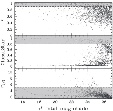
The objects were classified by performing the star-galaxy separation using three different parameters: ellipticity (=1 -b a); CLASS_STAR; and half-light radius (r1 2).

b/a is the axial ratio and CLASS_STAR is the SExtractor parameter associated with the light distribution of the detected objects. Galaxies are defined as those objects satisfying simultaneously ò <0.9; CLASS_STAR <0.8; and r1 2 > 5 pixels. Figure 6 shows an example of these parameters used to define the galaxies in the cluster [VMF98]124: ò, CLASS_STAR, and r1 2 in pixels as a function of r¢ total magnitudes. The adopted criteria allow us to remove spurious objects in the galaxy cluster fields, where saturated or overlapped objects in projection were among the most frequent problems.

We have adopted PSF magnitudes as the galaxy total magnitude and aperture magnitudes to obtain colors. Using the same aperture diameter for the whole galaxy cluster sample may introduce some systematic effects due to considering

different parts of the galaxies. We have used an aperture size equivalent to a diameter of 10 kpc at the cluster redshift for aperture magnitudes. This diameter is a compromise value that takes into account the typical galaxy size avoiding external contaminations.

3.2.2. Magnitude Calibration

In order to check the photometric calibration, objects classified as stars obtained with SExtractor in the observed images were compared with the USNO-A2.0 catalog (Monet et al.2003)for B, R, andImagnitudes; the NOMAD catalog (Zacharias et al.2005)forVmagnitudes and the Sloan Digital Sky Survey—DR12(Alam et al.2015, hereafter SDSS)forg¢,

¢

r, and i¢ magnitudes. In general, saturated stars or objects fainter than the catalog limiting magnitude were not used as possible misclassifications may contribute with inaccurate magnitudes, particularly at fainter levels. The galaxy cluster [VMF98]124 is not covered by the SDSS and we have first converted the USNO stellar magnitudes into the SDSS system using Fukugita et al. (1996) relations. Table 3 shows these magnitude offsets corresponding to the different observed passbands for each galaxy cluster. These values were taken into account for the final magnitudes and colors. The magnitudes are in the AB system and have been corrected for galactic extinction by using reddening maps from Schlegel et al.(1998) and the Cardelli et al.(1989)relations.

3.2.3. Limiting Magnitudes and Completeness

In order to check the SExtractor behavior at fainter magnitudes, we have estimated magnitude limits and com-pleteness levels using simulated catalogs and images created with the Astromatic packages STUFF and SKYMAKER (Bertin 2009). STUFF simulates field galaxy catalogs in a Poisson distribution, for different redshift slices from 0 < z < 20, with the number of galaxies and their absolute luminosities being taken from a non-evolving Schechter Luminosity Function (Schechter 1976). Galaxy profiles were modeled by the contribution of two components: a de Vaucouleurs bulge and an exponential disk (for details, see Erben et al.2001). The photometric, structural, and astrometric parameters for all objects were generated in all passbands using thefilter transmission curves and spectral energy distributions.

SKYMAKER produces realistic ground-based PSFs using STUFF catalogs taking into account the instrumentation and observing conditions.

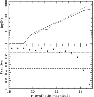
Using these packages, we have reproduced our observa-tions generating synthetic images and catalogs. We have run SExtractor in these simulated images and the resulting catalogs were compared with those created by SKYMAKER. Figure 7 shows an example of the number of object detections per magnitude bin (upper panel) obtained from the r¢ simulated catalog and those sources detected by SExtractor from the synthetic images. The distributions are shown in logarithmic scale as short and long dash lines, respectively. In the lower panel, the fraction of these detected distributions per magnitude bin are displayed

indicating the 50% and 90% completeness fractions. This figure indicates that the number of detections are similar; in this example, the SKYMAKER and SExtractor magnitudes are in good mutual agreement up tor¢of about 23 mag. For each galaxy cluster, the observing conditions were simulated with this procedure and magnitude limits were obtained. Table 4 shows the limiting magnitudes within 90% completeness.

As the magnitude errors provided by SExtractor are underestimated (White et al. 2005), our error estimates were based on the comparison between the synthetic magnitudes derived from SKYMAKER and those obtained with SEx-tractor. Within a 90% completeness level, the mean magnitude errors were found to be approximately 0.1 mag.

4. SPECTROSCOPY

4.1. Observations

The GMOS instrument was used in the MOS mode at the Gemini north and south telescopes during the SVP in 2003, under photometric conditions with typical seeing of about 0.6 and 0.9 arcsec. A GMOS grating of 400 lines/mm ruling density centered at 6700Å was used, covering a wavelength range of 4400 to 9800Å. The spectra had a resolution of about 5.5Å, with a dispersion of 1.37Å/pix, and offsets of ∼35Å were applied between exposures in the spectral direction toward the blue and/or the red tofill the gaps between CCDs.

The comparison lamp (CuAR) spectra were taken after each science exposure.

We have obtained spectroscopic data for galaxies in the fields of four galaxy clusters: [VMF98]022, [VMF98]097, [VMF98]102, and [VMF98]124. The spectroscopic targets were based on the photometric catalogs generated with SExtactor, as described in the previous section. In order to study cluster galaxy population, we selected objects brighter thanr¢ =23 mag, without any color criteria (Carrasco et al. 2007). Observations were performed with two masks for the clusters[VMF98]097 and[VMF98]102. Objects brighter than

¢

r=20 mag were observed in a single mask with shorter exposure time than the fainter ones. Table 5 shows the observed cluster identification, with a summary of the spectro-scopic observations including observation date, exposure time, and number of observed spectra per mask.

4.2. Data Reduction

The observations including comparison lamps and spectro-scopicflats were bias subtracted and trimmed using the Gemini IRAF package. The flats were processed by removing the calibration unit plus the GMOS spectral response and the calibration unit uneven illumination, which were then normal-ized to leave only the pixel-to-pixel variation and fringing.

Details of the reduction procedure are found in Carrasco et al.(2007).

The procedure to measure the galaxy radial velocity was started with an inspection of the galaxy spectra searching for strong features such as absorption and/or emission lines. RVIDLINES was applied for galaxies with clear emission lines, identifying one or more spectral lines and comparing with the rest-frame wavelengths. The average wavelength shifts were computed and converted to a radial velocity, with the residual of all shifts being used to estimate errors. In contrast, FXCOR was applied in early-type galaxies, cross-correlating the observed spectra with high signal-to-noise templates, with

Figure 6.The three adopted star-galaxy indicators vs.r¢total magnitudes. The gray zones indicate the typical regions where point sources are located. The dashed line marks our limit to separate galaxies and stars.

Table 3

Photometric Calibration: Magnitude Offsets

[VMF098] DB DV DR DI D ¢g D ¢r D ¢i

Id.

001 L L L L L −0.090±0.059 0.137±0.042

004 0.198±0.014 0.215±0.096 0.012±0.069 −0.274±0.052 L L L

011 0.040±0.007 L −0.102±0.024 L L L L

015 −0.113±0.010 0.101±0.032 −0.102±0.026 −0.224±0.023 L L L

022 L L L L L 0.276±0.019 −0.244±0.027

024 0.178±0.004 0.193±0.018 −0.111±0.038 0.268±0.039 L L L 025 0.212±0.011 0.177±0.046 −0.285±0.033 −0.099±0.006 L L L 045 0.030±0.091 −0.265±0.024 0.142±0.025 0.160±0.037 L L L 046 0.101±0.211 0.244±0.217 −0.137±0.021 −0.212±0.050 L L L

093 L L L L L 0.181±0.014 0.264±0.016

097 L L L L 0.221±0.089 0.299±0.061 L

102 L L L L L 0.114±0.091 L

113 0.052±0.511 0.091±0.055 0.103±0.018 0.099±0.027 L L L

119 L L L L L 0.049±0.084 0.040±0.101

124 L L L L 0.222±0.027 0.060±0.011 L

148 L L L L L 0.323±0.049 0.224±0.170

211 0.026±0.022 L 0.278±0.042 L L L L

theR-value(Tonry & Davis1979)used to define the quality of the measured radial velocities (Carrasco et al. 2007). For

>

R 3.5, the observed radial velocity was associated to the template that produced lower uncertainties. However, in the case ofR„3.5, absorption features were searched for and line-by-line Gaussian fits were obtained. Both RVIDLINES and FXCOR routines are part of the RV package in IRAF.

We have obtained radial velocities of objects selected in the neighborhoods of the four galaxy clusters and, for further analysis we need to know the completeness levels of their

magnitude distributions. For the photometric samples, the limiting magnitudes and completeness levels are extensively discussed in Section3.2.3. For the spectroscopy, the magnitude distributions of the clusters [VMF98]022, [VMF98]097 and [VMF98]102 show a brighter limiting magnitude ofr¢ ~20.5 mag, reaching a 90% completeness levels similar to the photometric samples. The cluster [VMF98]124 has been observed with only one mask with shorter exposure time, resulting in about 50% completeness at the same limiting magnitude.

5. CLUSTER MEMBERSHIP

In order to understand better the cluster assembly and morphological evolution of galaxies in low X-ray luminosity clusters, it is crucial to define cluster membership. Even when precise radial velocities are available for a large number of objects, the galaxy assignment of a cluster is not guaranteed. In effect, relatively distant infalling galaxies onto the cluster will appear closer to the cluster kinematic center. On the other hand, interlopers, namely, galaxies that are not confined to the cluster region may appear in projection with a low clustercentric relative velocity and therefore could be wrongly assigned as members. Using mock galaxy redshift surveys, van den Bosch et al.(2004)found that the velocity distribution of interlopers is strongly peaked toward the cluster mean radial velocity, thus introducing a bias in the cluster member assignment, especially at higher velocity dispersions.

We have selected galaxies within a projected radius of 0.75 Mpc from the X-ray emission peak. This choice is based on the angular size of the lowest redshift clusters and the available instrument FOVs. The relatively small radius minimizes foreground/background galaxy contamination and correspond to the densest cluster regions. It must be noted that by exploring the central regions of galaxy clusters, our study will focus on those galaxies mostly affected by the cluster environment at these redshifts. Thus, our analysis does not address the properties of galaxies far from the cluster core, which could be potentially different than those in the higher density regions.

5.1. Spectroscopic Membership and Substructures

In our cluster sample, only four galaxy clusters: [VMF98] 022, [VMF98]097, [VMF98]102 and [VMF98]124 have spectroscopic redshift measurements. The cluster membership was defined using the projected radius and also the spectro-scopic restrictionΔV<s, withΔVdefined as the difference between a given galaxy radial velocity and the cluster redshift given by Mullis et al.(2003). Testing membership assignment using 1 or 2σs show in general, small differences between the samples. However, there are some variations in the cluster [VMF98]097 with signs of a more complex morphology (Carrasco et al.2007; Nilo Castellón et al.2014). As previously mentioned, although membership cannot be totally guaranteed, we believe that the use of 1σ restriction is appropriate to minimize interlopers. The number of cluster members are shown in Column 5 of the Table5.

The bi-weight estimator (Beers et al. 1990) is statistically more robust and efficient for computing the central location of the redshift distribution than the standard mean. Biviano et al. (2006)have used this estimator for galaxy clusters with more than 15 members. We have obtained bi-weightσestimates for

Figure 7.Completeness levels using simulated data. The upper panel shows the SKYMAKER(short dash line)and SExtractor synthetic(long dash line) total magnitude distributions in logarithmic scale. In the lower panel, the ratio of these two distributions are shown. The two horizontal lines correspond to 50% and 90% completeness levels.

Table 4

Observed Magnitude Limits Within 90% Completeness Levels

the galaxy clusters with spectroscopic measurements. Using cluster members, columns 6 and 7 of Table5shows the mean redshift and the line of sight velocity dispersion obtained with this estimate. The uncertainties derived from a bootstrap resampling technique were approximately 0.001 for redshifts and 90 km s−1for velocity dispersions. We have also computed with cluster members, the mean redshift and velocity dispersion using the jackknife error estimates, which are shown in columns 8 and 9, respectively. We can see from this table that the velocity dispersion values using the two estimators are in agreement within the uncertainties, except for the galaxy cluster [VMF98]097. The higher value obtained using the jackknife estimate is a consequence of the complex cluster morphology. In the cluster [VMF98]124 which has only 12 galaxy members, we have also used the gapper statistics obtaining a highers~751 km s−1, which is in agreement with the other estimates.

Figure 8 shows the observed redshift distribution in the neighborhoods of the four galaxy clusters with available spectroscopy, where the shaded parts correspond to the distributions within 1σ of the mean cluster redshift. Gaussian function fits provide a suitable approximation to the line of sight distribution. The foreground and background structures are also present in thefigure. In the right corner, a detail of this distribution and the Gaussian fit are displayed. In the case of [VMF98]097, two peaks at redshifts 0.482 and 0.494 are clearly observed. This is the only galaxy cluster with well defined substructure, as also reported by Carrasco et al.(2007). For the cluster [VMF98]102, there is a second peak corresponding to a probable background system in the line of sight. On average, the uncertainties of the radial velocities were less than 55 km s−1.

5.2. Photometric Redshifts

The determination of cluster members using spectroscopic redshifts is certainly the most accurate method, but it is much more expensive in telescope time, especially at fainter magnitudes. Colors trace the spectral energy distribution of galaxies at different redshifts and the intersection of a given set of observed colors with the allowed redshift ranges can be used to assess the redshift of a galaxy. For this reason, redshift estimates of large and deep samples of galaxy clusters can be obtained by using broadband photometry.

Photometric redshift estimates have been widely used as an efficient way to study the galaxy properties using statistical tools (Koo 1985; Connolly et al. 1995; Gwyn & Hartwick 1996; Hogg et al. 1998; Fernández-Soto et al. 1999; Benítez

2000; Budavári et al.2000; Csabai et al.2000), as for example luminosity, colors and morphology. Even with larger uncer-tainties, they provide a powerful tool for studying evolutionary galaxy properties of faint galaxies. Two groups of methods are used to estimate photometric redshifts. The template fitting technique makes use of a small set of model galaxy spectra derived from the c2_{-based spectral template-fitting package}

(Bolzonella et al. 2000; Csabai et al. 2003). This approach consists in the reconstruction of the observed galaxy colors in order to find the best combination of template spectra at different redshifts. The main disadvantage of this method is the relatively small number of available templates in the library for different passbands. The second group is the empiricalfitting technique which is based on empirical data (Connolly et al. 1995; Brunner et al.1999; Collister & Lahav2004)requiring a large amount of a priori redshift information (training set), which may be in some cases a disadvantage. However, the main goal of this procedure is to obtain redshift estimates as a function of the photometric parameters as inferred from the training set.

We consider photometric redshift estimates (Photo-z) to assign membership for the fifteen galaxy clusters without spectroscopic measurements.

5.2.1. Photo-z with Annz

We have used the Artificial Neural Network (ANNz, Collister & Lahav2004), an empiricalfitting method to obtain photo-zas described in O’Mill et al. (2012). To calibrate the code, we have used 12,280 galaxies with spectroscopic redshifts derived from the Canadian Network for Observational Cosmology (Yee et al. 1996 CNOC). This data set was randomly divided into two subsamples, thereby generating the training and validation set.

The ANNz produces better estimates when more observa-tions in different passbands are available. We have used aperture magnitudes as defined in Section 3.2.1 for the nine galaxy clusters observed in four passbands: B V R, , , andI at the LCO and CTIO telescopes, defining a subsample of galaxies reaching the CNOC limiting magnitudes. The photometric resdhift estimates take into account the telescope characteristics and the adoptedfilters through the training and validation sets. The resulting ANNz architecture adopted here was 4:8:8:1. Therefore, they were obtained using the photo-metric catalogs and the distributions are related to the limiting magnitudes and completeness levels of these photometric samples(Section3.2.3). Abdalla et al.(2011)and Dahlen et al. (2013)have discussed associated bias and related uncertainties

Table 5

Spectroscopic Observations and Results

[VMF98] Observation Exposure Observed Member Mean Velocity Mean Velocity

Id. Date Time Spectra Galaxies Redshifta Dispersiona Redshiftb Dispersionb

in the photometric redshift estimates obtained with different methods by a comparison with spectroscopic measurements. Abdalla et al.(2011)have found that the ANNz method has an almost constant, small bias and a 1σscatter of about 0.06. The clusters[VMF98]011 and[VMF98]211 have been observed at LCO in only two passbands (B and R) and the photometric redshifts using ANNz are not accurate enough for our purposes of membership and they are not consider in this work.

5.2.2. Photo-z from the SDSS

The photometric data observed with the Gemini telescopes were obtained in two passbands; for the reasons mentioned above, determining photo-zwas not possible with the use of the ANNz method. For the galaxy clusters[VMF98]001,[VMF98] 093,[VMF98]119, and[VMF98]148 without spectroscopy, we have used photometric redshifts extracted from the PHOTOZ tables (http://skyserver.sdss.org/CasJobs) of the SDSS-DR8. These photometric redshifts use machine learning techniques with training sets, similar to those of ANNz. The SDSS is 95% complete for point sources up tor¢ ~22.2 mag. For the galaxy clusters in our sample with photometric redshifts from SDSS, the magnitude distributions are in agreement with the SDSS limiting magnitudes and completeness levels. In order to estimate photometric redshift uncertainties, which are signifi -cantly larger than spectroscopic measurements, we have made a

comparison with two galaxy clusters: [VMF98]022 and [VMF98]097 with both spectroscopic and photometric red-shifts. Figure 9 shows the comparisons between our spectro-scopic redshift estimates with the photometric redshifts from the SDSS-DR8. In the left panels, the projected distribution of objects with spectroscopic (empty squares) and photometric (filled circles)redshifts are shown within the 0.75 Mpc region represented by the dashed circles. The right panels correspond to the differenceszsp–zphSDSS as a function of zsp. The mean of these differences are−0.014±0.087 for[VMF98]022 and 0.033±0.063 for[VMF98]097, which are comparable to the uncertainties obtained by O’Mill et al. (2012). These mean values are represented with dashed lines and the 1σscatter by the gray region.

Since it is also seen that forΔV=6000 km s−1, contamina-tion is less than 10% with a still large number of true members, we have adopted this galaxy photometric redshift difference with respect to the cluster spectroscopic redshift in order to assess membership.

5.3. Membership Summary

Cluster members are then, the galaxies within a projected radius of 0.75 Mpc from the X-ray emission peak and with spectroscopic ΔV = 1σ or photometric ΔV ∼ 6000 km s−1. Mean values of the cluster redshift with the members were

obtained and the comparison with Mullis et al. (2003) gives mean differences of about 0.002±0.005. Table6 shows the final membership summary with the number of members assigned to the clusters in column 2, our mean redshift estimates in column 3 and the redshift source in column 4. Our spectroscopic measurements are identified as zsp while our photometric estimates withzphand the SDSS estimates withzph SDSS. As mentioned above, we could not obtain the galaxy members of the clusters [VMF098]011 and [VMF098]211 because they have been observed in only two passbands. Also, the clusters [VMF098]024 and [VMF098]025 have redshifts similar to some members in common (see Figure 3).

6. FINAL COMMENTS AND FUTURE PLANS

Our project is centered on the study of low X-ray luminosity clusters of galaxies at intermediate redshifts and the analysis of the morphological galaxy content. At the end of the project, the photometric and spectroscopic data will be available athttp:// astro.userena.cl/science/LowXrayClusters/.

This paper presents our sample and main goals. Nineteen galaxy clusters were selected with X-ray luminosities ofLX~ 0.5–45×1043erg s−1 in the redshift range of 0.16–0.70, which were observed at LCO, CTIO, and Gemini Observatory with different instruments and passbands. We extensively

Figure 9. Spectroscopic and photometric redshift comparison. Upper panels show the projected distribution of galaxies in the[VMF98]022field(left)and the differences between spectroscopic and photometric redshift estimates vs. spectroscopic values(right). In this panel, the mean value is represented by a dashed line and the 1σscatter correspond to the gray region. Lower panels are the same for galaxies in the cluster[VMF98]097.

Table 6

Member Assignment for the Sample of Low X-Ray Galaxy Clusters

[VMF98] Number of Our Mean Redshift Redshift

Id. Cluster Members Source

001 22 0.495 zphSDSS

004 32 0.292 zph

011 L L L

015 44 0.249 zph

022 26 0.247 zsp∣zphSDSS

024 51 0.168 zph

025 46 0.163 zph

045 29 0.292 zph

046 38 0.200 zph

093 14 0.357 zphSDSS

097 37 0.482 zsp∣zphSDSS

102 22 0.409 zsp

113 35 0.258 zph

119 20 0.692 zphSDSS

124 12 0.185 zsp

148 16 0.697 zphSDSS

211 L L L

214 41 0.198 zph

discussed the photometric and spectroscopic observations and the data reduction, which includes the galaxy identification and cluster membership together with the spectroscopic and photometric redshifts and their error estimates.

The second paper of the series (Nilo Castellón et al.2014) considered the optical properties and morphological content of the seven galaxy clusters observed with Gemini north and south telescopes at 0.18 <z<0.70. The main results are an increment of the blue galaxy fraction and a reduction of the lenticular fraction with redshifts. The early-type fraction remains almost constant in the whole redshift range. These results are in agreement with those observed for massive clusters.

The third paper of the series(Gonzalez et al.2015)presented the weak lensing analysis of the galaxy clusters observed with Gemini telescopes. We determined the masses of seven galaxy clusters, six of which were measured for the first time. The weak lensing mass determinations correlate with the X-ray luminosities following the observed M–LXrelation.

In forthcoming papers, we will present several analyses of the data, such us the galaxy Luminosity Function, the RCS, density profiles, and morphological content. In C. Valotto et al. (2016, in preparation), we will take advantage of the photometric data and cluster membership to study the luminosity function of the galaxy cluster sample with different X-ray luminosities in the redshift range of 0.18–0.70. Also, M. V. Alonso et al. (2016, in preparation) will present an analysis of the CMDs, the RCS, color–color diagrams, and density profiles for the galaxy clusters observed at LCO and CTIO in the redshift range of 0.16–0.30. Finally, in H. Cuevas et al. (2016, in preparation), we will study the morphological evolution taking into account the 19 galaxy clusters in the sample.

A second part of this project includes more spectroscopic measurements, which will allow us to search for substructures and global cluster dynamics. The combination of photometric and spectroscopic data analysis could provide useful hints to trace the evolutionary scenario of these low X-ray galaxy clusters.

J.L.N.C., M.J., and F.R. acknowledge the financial support from Consejo Nacional de Investigaciones Científicas y Técnicas de la República Argentina (CONICET). This work was partially supported by grants by CONICET, Secretaría de Ciencia y Técnica(Secyt)of Universidad Nacional de Córdoba and Ministerio de Ciencia y Tecnología (MINCyT, Córdoba). J.L.N.C. also acknowledges financial support from the Dirección de Investigación de la Universidad de La Serena (DIULS), the Programa de Incentivo a la Investigación Académica, Programa DIULS de Iniciacin Cientfica PI15142, and from ALMA-CONICYT postdoctoral program No. 31120026. H.C. acknowledges support by Dirección de Investigación de la Universidad de La Serena, PR13143.

SDSS-III is managed by the Astrophysical Research Consortium for the Participating Institutions of the SDSS-III Collaboration including the University of Arizona, the Brazilian Participation Group, Brookhaven National Labora-tory, University of Cambridge, University of Florida, the French Participation Group, the German Participation Group, the Instituto de Astrofísica de Canarias, the Michigan State/ Notre Dame/JINA Participation Group, Johns Hopkins Uni-versity, Lawrence Berkeley National Laboratory, Max Planck

Institute for Astrophysics, New Mexico State University, New York University, Ohio State University, Pennsylvania State University, University of Portsmouth, Princeton University, the Spanish Participation Group, University of Tokyo, University of Utah, Vanderbilt University, University of Virginia, University of Washington, and Yale University.

REFERENCES

Abdalla, F. B., Banerji, M., Lahav, O., & Rashkov, V. 2011, MNRAS, 417, 1891

Alam, S., Albareti, F. D., Allende Prieto, C., et al. 2015,ApJS,219, 12 Baldry, I. K., Glazebrook, K., Brinkmann, J., et al. 2004,ApJ,600, 681 Balogh, M., Bower, R. G., Smail, I., et al. 2002,MNRAS,337, 256 Balogh, M. L., McGee, S. L., Wilman, D. J., et al. 2011,MNRAS,412, 2303 Beers, T. C., Flynn, K., & Gebhardt, K. 1990,AJ,100, 32

Benítez, N. 2000,ApJ,536, 571

Berrier, J. C., Stewart, K. R., Bullock, J. S., et al. 2009,ApJ,690, 1292 Bertin, E. 2009, MSAIS,80, 422

Bertin, E. 2011, adass XX,442, 435

Bertin, E., & Arnouts, S. 1996, A&AS,117, 393

Biviano, A., Murante, G., Borgani, S., et al. 2006,A&A,456, 23 Blanton, M. R., & Moustakas, J. 2009,ARA&A,47, 159 Bolzonella, M., Miralles, J.-M., & Pelló, R. 2000, A&A,363, 476

Brunner, R. J., Djorgovski, S. G., Gal, R. R., & Odewahn, S. C. 1999, BAAS, 31, 1492

Budavári, T., Szalay, A. S., Connolly, A. J., Csabai, I., & Dickinson, M. 2000, AJ,120, 1588

Butcher, H., & Oemler, A., Jr. 1984,ApJ,285, 426

Cardelli, J. A., Clayton, G. C., & Mathis, J. S. 1989,ApJ,345, 245 Carrasco, E. R., Cypriano, E. S., Neto, G. B. L., et al. 2007,ApJ,664, 777 Christlein, D., & Zabludoff, A. I. 2005,ApJ,621, 201

Collister, A. A., & Lahav, O. 2004,PASP,116, 345

Connelly, J. L., Wilman, D. J., Finoguenov, A., et al. 2012,ApJ,756, 139 Connolly, A. J., Csabai, I., Szalay, A. S., et al. 1995,AJ,110, 2655 Csabai, I., Budavári, T., Connolly, A. J., et al. 2003,AJ,125, 580 Csabai, I., Connolly, A. J., Szalay, A. S., & Budavári, T. 2000,AJ,119, 69 Dahlen, T., Mobasher, B., Faber, S. M., et al. 2013,ApJ,775, 93

De Lucia, G., Poggianti, B. M., Aragón-Salamanca, A., et al. 2004,ApJL, 610, L77

Dressler, A. 1980,ApJS,42, 565

Dressler, A., & Gunn, J. E. 1992,ApJS,78, 1

Erben, T., Van Waerbeke, L., Bertin, E., Mellier, Y., & Schneider, P. 2001, A&A,366, 717

Fernández-Soto, A., Lanzetta, K. M., & Yahil, A. 1999,ApJ,513, 34 Finn, R. A., Zaritsky, D., McCarthy, D. W., Jr.,, et al. 2005,ApJ,630, 206 Fukugita, M., Ichikawa, T., Gunn, J. E., et al. 1996,AJ,111, 1748 Gilbank, D. G., Yee, H. K. C., Ellingson, E., et al. 2008,ApJ,673, 742 Girardi, M., & Mezzetti, M. 2001,ApJ,548, 79

Gladders, M. D., Lopez-Cruz, O., Yee, H. K. C., & Kodama, T. 1998,ApJ, 501, 571

Gonzalez, E. J., Foëx, G., Nilo Castellón, J. L., et al. 2015,MNRAS,452, 2225 Gunn, J. E., & Gott, J. R., III 1972,ApJ,176, 1

Gwyn, S. D. J., & Hartwick, F. D. A. 1996,ApJL,468, L77 Hogg, D. W., Cohen, J. G., Blandford, R., et al. 1998,AJ,115, 1418 Hook, I. M., Jørgensen, I., Allington-Smith, J. R., et al. 2004, PASP,

116, 425

Jeltema, T. E., Mulchaey, J. S., Lubin, L. M., Rosati, P., & Böhringer, H. 2006, ApJ,649, 649

Jensen, P. C., & Pimbblet, K. A. 2012,MNRAS,422, 2841 Kauffmann, G., & Charlot, S. 1998,MNRAS,294, 705

Kodama, T., Arimoto, N., Barger, A. J., & Aragón-Salamanca, A. 1998, A&A, 334, 99

Koo, D. C. 1985,AJ,90, 418 Landolt, A. U. 1992,AJ,104, 340

Lerchster, M., Seitz, S., Brimioulle, F., et al. 2011,MNRAS,411, 2667 Lubin, L. M., Gal, R. R., Lemaux, B. C., Kocevski, D. D., & Squires, G. K.

2009,AJ,137, 4867

Mendez, A. J., Coil, A. L., Lotz, J., et al. 2011,ApJ,736, 110 Monet, D. G., Levine, S. E., Canzian, B., et al. 2003,AJ,125, 984 Mulchaey, J. S., Lubin, L. M., Fassnacht, C., Rosati, P., & Jeltema, T. E. 2006,

ApJ,646, 133

Mullis, C. R., McNamara, B. R., Quintana, H., et al. 2003,ApJ,594, 154 Nilo Castellón, J. L., Alonso, M. V., Lambas, D. G., et al. 2014,MNRAS,

Oemler, A., Jr., Dressler, A., Gladders, M. G., et al. 2013,ApJ, 770, 61 O’Mill, A. L., Duplancic, F., García Lambas, D., Valotto, C., & Sodré, L.

2012,MNRAS,421, 1897

Piffaretti, R., Arnaud, M., Pratt, G. W., Pointecouteau, E., & Melin, J.-B. 2011, A&A,534, A109

Popesso, P., Biviano, A., Böhringer, H., Romaniello, M., & Voges, W. 2005, A&A,433, 431

Rosati, P., Stanford, S. A., Eisenhardt, P. R., et al. 1999,AJ,118, 76 Schechter, P. 1976,ApJ,203, 297

Schlegel, D. J., Finkbeiner, D. P., & Davis, M. 1998,ApJ,500, 525 Spitzer, L., Jr., & Baade, W. 1951,ApJ, 113, 413

Stott, J. P., Smail, I., Edge, A. C., et al. 2007,ApJ,661, 95

Strazzullo, V., Rosati, P., Pannella, M., et al. 2010,A&A,524, A17 Tody, D. 1993, adass II,52, 173

Tonry, J., & Davis, M. 1979,AJ,84, 1511

van den Bosch, F. C., Norberg, P., Mo, H. J., & Yang, X. 2004,MNRAS, 352, 1302

Vikhlinin, A., McNamara, B. R., Forman, W., et al. 1998,ApJ,502, 558 Wake, D. A., Collins, C. A., Nichol, R. C., Jones, L. R., & Burke, D. J. 2005,

ApJ,627, 186