TítuloMapping chemical structure activity information of HAART drug cocktails over complex networks of AIDS epidemiology and socioeconomic data of U S counties
25
0
0
Texto completo
(2) 1. Introduction Computational algorithms may play an important role in the process of elucidation of structure– activity relationships for many molecular systems and biological problems (Aguilera and RodriguezGonzalez, 2014, Barresi et al., 2013, Gonzalez-Diaz et al., 2011 and Munteanu et al., 2009). In particular, the theoretical biology has been useful in the study of anti-HIV drugs and/or their molecular targets (Jain Pancholi et al., 2014, Ogul, 2009, Speck-Planche et al., 2012, Weekes and Fogel, 2003 and Xu et al., 2013). However, classic algorithms useful to connect the structure of a single molecule with its biological properties are unable to study the effect of combinations (cocktails) of drugs over epidemiological outbreaks in large populations with different social and economic factors. For instance, infections with HIV are commonly treated with antiretroviral drug combinations. These treatments could diminish the risk of HIV transmission (Castilla et al., 2005 and Ping et al., 2013). In addition, the rates of disease progression, opportunistic infections, and mortality decreased with the implementation of HAART, and the combination of anti-HIV drugs resulted in longer survival and a better quality of life for the people infected with the virus (Colombo et al., 2014). The most common drug treatment administered to patients consists of two nucleoside reverse transcriptase inhibitors combined with either a non-nucleoside reverse transcriptase inhibitor, a “boosted” protease inhibitor or integrase strand transfer inhibitors (INSTIs), which resulted in decreased HIV RNA levels (<50 copies/mL) at 48 weeks and CD4 cell increases in the majority of patients (Usach et al., 2013). Research indicates (McMahon et al., 2011) that despite HAART therapy, HIV infected individuals who are poor, homeless, hungry, or have less education, continue to have a higher risk of death. Additionally, researchers (McMahon et al., 2011) suggest that HIV-infected individuals of low socioeconomic status (SES) are more likely to have increased mortality rates than those who are not living under these adverse conditions. Therefore, resources for HIV testing care and proven economic interventions should be directed to areas of economically disadvantaged people (McDavid Harrison et al., 2008). The case of the United States (U.S.) is interesting for theoretical studies due to the abundance of epidemiological information. Holtgrave and Crosby (2003) found an important correlation (r = 0.469, p < 0.01) between the income inequality and the AIDS case rates at state level in the U.S. In addition, in 2010, the U.S. National HIV Behavioural Surveillance System developed a study about HIV infection among heterosexuals at increased risk, involving a total of 12,478 persons. Out of 8473 participants, 197 (2.3%) participants were positive for HIV infection, and prevalence was similar for men (2.2%) and women (2.5%). The research study shows a higher prevalence in persons who reported less than a high school education (3.1%), compared with those with a high school education (1.8%). Income inequality, employment, and other social variables also seem to be relevant on AIDS epidemiology. Prevalence was also higher in those with an annual household income of less than $10,000 (2.8%), compared to those with an income of $20,000 or more (1.2%) (CDC, 2013). Moreover, the percentage of HIV-infected individuals was higher in participants who reported being unemployed (1.1%) or disabled (and unemployed) (2.7%), compared to employed (0.4%) ones. Some authors, such as Mondal and Shitan (2013), commented in their study connections among life expectancy, income, educational attainment, fertility, health facilities, and HIV prevalence. Recently, large amounts of data have been accumulated in public databases about the scope of molecular biology. For instance, the ChEMBL database (https://www.ebi.ac.uk/chembl/) (Bento et al., 2013, Gaulton et al., 2012 and Heikamp and Bajorath, 2011) provides data from life science experiments (Bento et al., 2013). In the same way, there are online resources containing epidemiological data of AIDS prevalence and data about socioeconomic factors at county level. These databases are AIDSVu (http://aidsvu.org), created by researchers at the Rollins School of Public Health at Emory University, and the U.S. Center for Disease Control and Prevention (CDC). In this context, the search of computational chemistry algorithms that may prove useful to carry out a mapping of structure–activity data of HAARTdrug cocktails over AIDS epidemiology networks and socioeconomic data is of major importance. In a recent paper (González-Díaz et al., 2014), ANNs have been used to link data related to AIDS in the U.S. counties to ChEMBL data about the chemical structure and preclinical activity of anti-HIV compounds. ANNs are prediction models, widely used in many areas of science, such as medicine, chemistry, biochemistry, as well as in drug development. In the latter, they are very useful for the prediction of properties of potential drugs. ANNs approximate the operation of the human brain with the ability to get results from complicated or imprecise data, which are very difficult to appreciate by humans or other computer techniques (Burbidge et al., 2001, Guha, 2013, Patel, 2013 and Speck-Planche et al., 2012). Indices of social networks and molecular graphs were used as input information. A Shannon information index based on the Gini coefficient was employed to quantify the effect of income inequality in the social network. In addition, Balaban’s information indices were used to quantify changes in the chemical structure of single anti-HIV drugs. Last, Box–Jenkins moving average operators (MA) were also.
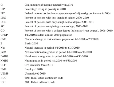
(3) employed to quantify information about the deviations of drugs with respect to data subsets of reference (targets, organisms, experimental parameters, protocols). In our previous paper (González-Díaz et al., 2014), the model found was able to link the deviations in the AIDS prevalence rates in the ath county to the changes in the biological activity of the qth drug (dq). However, the previous computational chemistry algorithm fails in accounting for drug cocktails and many socioeconomic factors. This work is aimed at developing, for the first time, a computational algorithm for network epidemiology which is able to map structure–activity data of HAART-drugs cocktails over complex networks of AIDS epidemiology and socioeconomic factors for >2000 U.S. counties.. 2. Materials and methods 2.1. Socioeconomic factors 2.1.1. Socioeconomic variables and Shannon-entropy transformation into information indices In total, 17 variables were withdrawn from AIDSVu, U.S. Census Bureau databases (http://www.census.gov/) and Internal Revenue Service (2014) (http://taxfoundation.org/). See the symbols and details of these variables in Table 1. All 17 socioeconomic variables (va) discussed previously come from very different original sources, describe different phenomena, and then use different scales.. Table 1. U.S. socioeconomic variables. County variables (v) Description. G. Gini measure of income inequality in 2010. LIP. Percentage living in poverty in 2010. FIT. Federal income tax burden as a percentage of adjusted gross income in 2004. LHS. Percent of persons with less than high school 2006–2010. OHS. Percent of persons with only a high school degree 2006–2010. SC. Percent of persons completing some college, 2006–2010. CD. Percent of persons with a college degree (at least a 4 year degree), 2006–2010. CPOP. 4/1/2010 resident Census 2010 population. ChR. Numeric change in resident total population 4/1/2010 to 7/1/2010. B. Births 2010. Nat. Natural increase in period 4/1/2010 to 6/30/2010. IntM. Net international migration in period 4/1/2010 to 6/30/2010. DMIG. Net domestic migration in period 4/1/2010 to 6/30/2010. NMIG. Net migration in period 4/1/2010 to 6/30/2010. CLF. Civilian labor force 2010. EMP. Employed 2010. UEMP. Unemployed 2010. RUC. 2003 Rural urban continuum code. UIC. 2003 Urban influence code. Less than high school (LHS): in 1990, 2000, 2006–2010 the share includes those who did not receive a high school diploma or its equivalent (such as a GED), but did not report college experience. Only high school degree (OHS): in 1990, 2000, and 2006–2010 the share includes those who completed 12th grade and received a high school diploma or its equivalent (such as a GED), but did not report college experience. Some college (SC): in 1990, 2000, and 2006–2010 the share includes those who reported completing at least one year of college but did not receive a bachelor’s degree. College graduate (CD): in 1990, 2000, and 2006–2010 the share includes those who received a bachelor’s or higher degree..
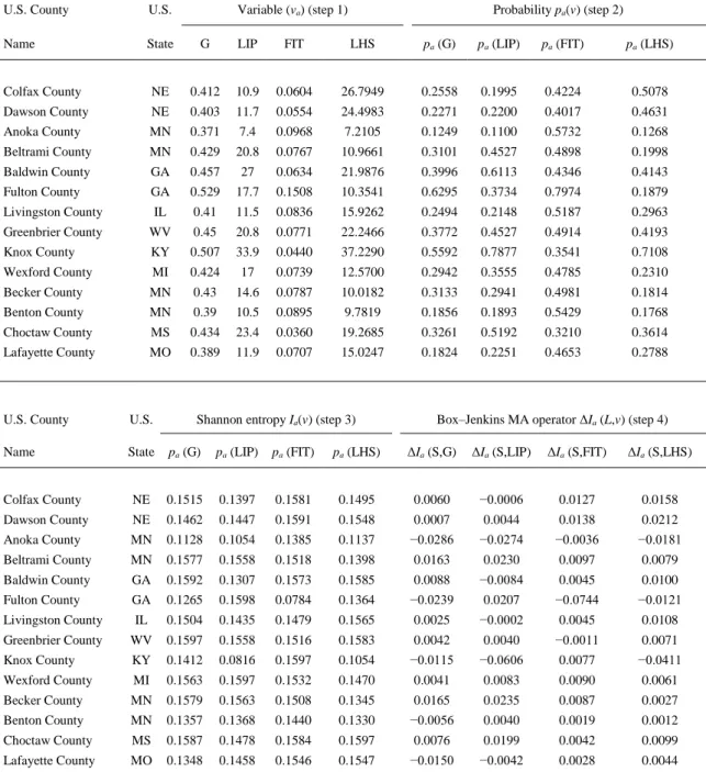
(4) In order to perform an uniform and scale unbiased representation of information, all these variables were transformed into Shannon entropy information indices Ia(v). These information indices depend on the values of variables rescaled into probabilities as follows: 𝐼𝑎 (𝑣) = −𝑝𝑎 (𝑣) × log𝑝𝑎 (𝑣) 𝑝𝑎 (𝑣) = (. 𝑣 − 𝑣min + 𝜖 ) 𝑣max − 𝑣min + 𝜖. This transformation guarantees that the new probability values become 1 for the maximum value (vmax) and approach to 0 for values close to minimum value (vmin). The scaling parameter ϵ = 0.0001 was used to avoid values of pa(v) = 0 with the subsequent undefined results of the entropy function for logarithm log (0). Table 2 shows a short example of the results of the consecutive probability and Shannon entropy scaling procedures for some variables.. 2.1.2. Demographic scale levels of socioeconomic information indices The variability of these 17 socioeconomic variables was studied on two different demographic scales. One of them refers to the geopolitical level and the other to the local population structure level. The first level was identified as the grouping of counties into 51 different states. Actually, there are only 47 states in our dataset. The second level was measured with two alternative codes: rural-urban continuum codes (RUCC), which distinguishes metropolitan counties by the population size of their metro area and nonmetropolitan counties by degree of urbanization and adjacency to a metro area. However, in this work the 2003 RUCC classification was used to preserve causality relationships. 2003 RUCC is the classification reported prior to the AIDSVu epidemic data, which is from 2010, and 2013 RUCC, which is posterior and could cause–effect relationships. The standard Office of Management and Budget (OMB) metro and nonmetro categories were subdivided into three metro and six nonmetro categories. Each county in the U.S. is assigned with one of the nine codes. This scheme allows researchers to break county data into finer residential groups, beyond metro and nonmetro, particularly for the analysis of trends in nonmetro areas that are related to population density and metro influence. In addition, the urban influence codes (UIC) distinguish metropolitan counties by population size of their metro area, and nonmetropolitan counties by size of the largest city or town and proximity to metro and micropolitan areas. The OMB metro and nonmetro categories were subdivided into two metro and 10 non-metro categories, resulting in a 12-part county classification. Table 3 shows the RUCC and UIC classification codes..
(5) Table 2. Process of transformation of original socioeconomic variables into MA operators. U.S. County. U.S.. Variable (va) (step 1). Probability pa(v) (step 2). Name. State. G. LIP. FIT. LHS. pa (G). pa (LIP). pa (FIT). pa (LHS). Colfax County. NE. 0.412. 10.9. 0.0604. 26.7949. 0.2558. 0.1995. 0.4224. 0.5078. Dawson County. NE. 0.403. 11.7. 0.0554. 24.4983. 0.2271. 0.2200. 0.4017. 0.4631. Anoka County. MN. 0.371. 7.4. 0.0968. 7.2105. 0.1249. 0.1100. 0.5732. 0.1268. Beltrami County. MN. 0.429. 20.8. 0.0767. 10.9661. 0.3101. 0.4527. 0.4898. 0.1998. Baldwin County. GA. 0.457. 27. 0.0634. 21.9876. 0.3996. 0.6113. 0.4346. 0.4143. Fulton County. GA. 0.529. 17.7. 0.1508. 10.3541. 0.6295. 0.3734. 0.7974. 0.1879. Livingston County. IL. 0.41. 11.5. 0.0836. 15.9262. 0.2494. 0.2148. 0.5187. 0.2963. Greenbrier County. WV. 0.45. 20.8. 0.0771. 22.2466. 0.3772. 0.4527. 0.4914. 0.4193. Knox County. KY. 0.507. 33.9. 0.0440. 37.2290. 0.5592. 0.7877. 0.3541. 0.7108. Wexford County. MI. 0.424. 17. 0.0739. 12.5700. 0.2942. 0.3555. 0.4785. 0.2310. Becker County. MN. 0.43. 14.6. 0.0787. 10.0182. 0.3133. 0.2941. 0.4981. 0.1814. Benton County. MN. 0.39. 10.5. 0.0895. 9.7819. 0.1856. 0.1893. 0.5429. 0.1768. Choctaw County. MS. 0.434. 23.4. 0.0360. 19.2685. 0.3261. 0.5192. 0.3210. 0.3614. Lafayette County. MO. 0.389. 11.9. 0.0707. 15.0247. 0.1824. 0.2251. 0.4653. 0.2788. Shannon entropy Ia(v) (step 3). Box–Jenkins MA operator ΔIa (L,v) (step 4). U.S. County. U.S.. Name. State. pa (G). pa (LIP). pa (FIT). pa (LHS). ΔIa (S,G). ΔIa (S,LIP). ΔIa (S,FIT). ΔIa (S,LHS). Colfax County. NE. 0.1515. 0.1397. 0.1581. 0.1495. 0.0060. −0.0006. 0.0127. 0.0158. Dawson County. NE. 0.1462. 0.1447. 0.1591. 0.1548. 0.0007. 0.0044. 0.0138. 0.0212. Anoka County. MN. 0.1128. 0.1054. 0.1385. 0.1137. −0.0286. −0.0274. −0.0036. −0.0181. Beltrami County. MN. 0.1577. 0.1558. 0.1518. 0.1398. 0.0163. 0.0230. 0.0097. 0.0079. Baldwin County. GA. 0.1592. 0.1307. 0.1573. 0.1585. 0.0088. −0.0084. 0.0045. 0.0100. Fulton County. GA. 0.1265. 0.1598. 0.0784. 0.1364. −0.0239. 0.0207. −0.0744. −0.0121. Livingston County. IL. 0.1504. 0.1435. 0.1479. 0.1565. 0.0025. −0.0002. 0.0045. 0.0108. Greenbrier County. WV. 0.1597. 0.1558. 0.1516. 0.1583. 0.0042. 0.0040. −0.0011. 0.0071. Knox County. KY. 0.1412. 0.0816. 0.1597. 0.1054. −0.0115. −0.0606. 0.0077. −0.0411. Wexford County. MI. 0.1563. 0.1597. 0.1532. 0.1470. 0.0041. 0.0083. 0.0090. 0.0061. Becker County. MN. 0.1579. 0.1563. 0.1508. 0.1345. 0.0165. 0.0235. 0.0087. 0.0027. Benton County. MN. 0.1357. 0.1368. 0.1440. 0.1330. −0.0056. 0.0040. 0.0019. 0.0012. Choctaw County. MS. 0.1587. 0.1478. 0.1584. 0.1597. 0.0076. 0.0199. 0.0042. 0.0099. Lafayette County. MO. 0.1348. 0.1458. 0.1546. 0.1547. −0.0150. −0.0042. 0.0028. 0.0044.
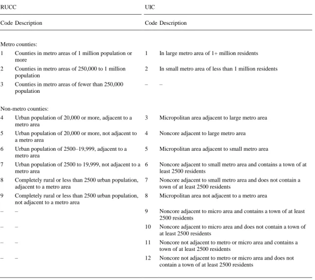
(6) Table 3. Values of the RUCC and UIC codes in the U.S. in 2003. RUCC. UIC. Code Description. Code Description. Metro counties: 1. Counties in metro areas of 1 million population or more. 1. In large metro area of 1+ million residents. 2. Counties in metro areas of 250,000 to 1 million population. 2. In small metro area of less than 1 million residents. 3. Counties in metro areas of fewer than 250,000 population. –. –. Non-metro counties: 4. Urban population of 20,000 or more, adjacent to a metro area. 3. Micropolitan area adjacent to large metro area. 5. Urban population of 20,000 or more, not adjacent to a metro area. 4. Noncore adjacent to large metro area. 6. Urban population of 2500–19,999, adjacent to a metro area. 5. Micropolitan area adjacent to small metro area. 7. Urban population of 2500 to 19,999, not adjacent to a 6 metro area. Noncore adjacent to small metro area and contains a town of at least 2500 residents. 8. Completely rural or less than 2500 urban population, adjacent to a metro area. 7. Noncore adjacent to small metro area and does not contain a town of at least 2500 residents. 9. Completely rural or less than 2500 urban population, not adjacent to a metro area. 8. Micropolitan area not adjacent to a metro area. –. –. 9. Noncore adjacent to micro area and contains a town of at least 2500 residents. –. –. 10. Noncore adjacent to micro area and does not contain a town of at least 2500 residents. –. –. 11. Noncore not adjacent to metro or micro area and contains a town of at least 2500 residents. –. –. 12. Noncore not adjacent to metro or micro area and does not contain a town of at least 2500 residents. 2.1.3. Box–Jenkins MA operators of socioeconomic variables at different levels The moving average operators of Box–Jenkins (MA) were used in order to measure the variability of the Ia(v) on two different demographic scales (state and population). In so doing, the average parameters <Ia(v)L> were calculated for different levels of population L = u, r, s. Consequently, the average values <Ia(v)s>, <Ia(v)r>, <Ia(v)u> were obtained for all the Ia(v) values. The parameters <Ia(v)s> are the averages of Ia(v) for all the counties in the same state (L = s). The parameters <Ia(v)r> are the averages of Ia(v) for all the counties with the same population structure according to the RUCC code (L = r). The parameters <Ia(v)u> are the averages of Ia(v) for all the counties with the same population structure according to the UIC code (L = u) ( Brown et al., 1976 and Ghelfi and Parker, 1997). After calculating the averages <Ia(v)L>, the values of the MA operators were determined for each county. The values of <Ia(v)s> were tabulated for 47 states. The values of <Ia(v)r> and <Ia(v)u> were also calculated for 9 and 12 different types of population structures according to the RUCC and UIC codes, respectively (see Table SM1 of Supplementary material). Some examples of MA operators for selected counties at State, RUCC, and UIC levels are shown in Table 4, see also other examples at state level in the last columns of Table 2.The formulae of these MA operators are: Δ𝐼𝑎 (𝑣)𝐿 = 𝐼𝑎 (𝑣) − 〈𝐼𝑎 (𝑣)𝐿 〉. Δ𝐼𝑎 (𝑣)𝑟 = 𝐼𝑎 (𝑣) − 〈𝐼𝑎 (𝑣)𝑟 〉. Δ𝐼𝑎 (𝑣)𝑠 = 𝐼𝑎 (𝑣) − 〈𝐼𝑎 (𝑣)𝑠 〉. Δ𝐼𝑎 (𝑣)𝑢 = 𝐼𝑎 (𝑣) − 〈𝐼𝑎 (𝑣)𝑢 〉.
(7) Table 4. Examples of MA operators for different scales and population structures for the selected counties U.S. County name. U.S. state. ΔIa (L,v). AIDSCR ΔIa (S,G)s. ΔIa (S,LIP)s. ΔIa (S,FIT)s. ΔIa (S,LHS)s. Perry County. PA. 71. −0.066. −0.012. 0.009. 0.007. Sedgwick County. KS. 177. 0.011. 0.011. −0.016. 0.012. Mercer County. PA. 66. 0.004. 0.014. 0.004. 0.002. Montgomery County. KS. 50. 0.006. 0.012. 0.006. 0.017. Westmoreland County. PA. 47. 0.007. −0.010. −0.006. −0.021. Boyd County. KY. 112. 0.004. 0.017. −0.015. 0.010. Northampton County. PA. 153. 0.003. −0.008. −0.009. 0.002. Riley County. KS. 59. 0.007. 0.008. −0.009. −0.034. Montgomery County. PA. 140. 0.008. −0.066. −0.056. −0.031. Pottawatomie County. KS. 48. 0.006. −0.023. 0.002. −0.019. Lebanon County. PA. 101. −0.006. −0.006. 0.004. 0.009. Monroe County. PA. 173. −0.007. 0.005. 0.004. −0.005. Wyoming County. PA. 45. −0.013. 0.004. 0.003. −0.007. Boyle County. KY. 89. 0.001. 0.017. −0.006. 0.012. County Name. State. AIDSCR. ΔIa (R,G). ΔIa (R,LIP). ΔIa (R,FIT). ΔIa (R,LHS). Perry County. PA. 71. −0.066. −0.014. 0.010. 0.009. Sedgwick County. KS. 177. 0.008. 0.010. −0.008. 0.002. Mercer County. PA. 66. 0.004. 0.012. 0.005. 0.004. Montgomery County. KS. 50. 0.004. 0.015. 0.009. 0.009. Westmoreland County. PA. 47. 0.013. 0.002. 0.005. −0.015. Boyd County. KY. 112. 0.004. 0.011. −0.005. 0.013. Northampton County. PA. 153. 0.003. −0.010. −0.009. 0.005. Riley County. KS. 59. 0.004. 0.011. −0.006. −0.042. Montgomery County. PA. 140. 0.014. −0.054. −0.046. −0.025. Pottawatomie County. KS. 48. 0.004. −0.023. −0.002. −0.034. Lebanon County. PA. 101. −0.007. −0.010. 0.000. 0.010. Monroe County. PA. 173. −0.008. 0.002. −0.002. −0.007. Wyoming County. PA. 45. −0.013. 0.002. 0.003. −0.005. Boyle County. KY. 89. 0.002. 0.017. −0.005. 0.014. County Name. State. AIDSCR. ΔIa (U,G). ΔIa (U,LIP). ΔIa (U,FIT). ΔIa (U,LHS). Perry County. PA. 71. −0.066. −0.015. 0.007. 0.009. Sedgwick County. KS. 177. 0.008. 0.009. −0.010. 0.001. Mercer County. PA. 66. 0.003. 0.011. 0.002. 0.003. Montgomery County. KS. 50. 0.003. 0.015. 0.006. 0.007. Westmoreland County. PA. 47. 0.013. 0.002. 0.005. −0.015. Boyd County. KY. 112. 0.004. 0.010. −0.007. 0.012. Northampton County. PA. 153. 0.002. −0.011. −0.011. 0.004. Riley County. KS. 59. 0.003. 0.011. −0.008. −0.044. Montgomery County. PA. 140. 0.014. −0.054. −0.046. −0.025. Pottawatomie County. KS. 48. 0.004. −0.022. 0.001. −0.033. Lebanon County. PA. 101. −0.007. −0.009. 0.002. 0.011. Monroe County. PA. 173. −0.008. 0.000. −0.003. −0.009. Wyoming County. PA. 45. −0.014. 0.001. 0.001. −0.005.
(8) 2.2. Biomolecular factors 2.2.1. Shannon-entropy transformation of chemical structure into information indices Quantitative descriptors of the drug molecular graph can be used to quantify the chemical structure of anti-HIV compounds. The molecular information indices Id(k) implemented in the software DRAGON, version 5.3 ( Todeschini and Consonni, 2000) were employed; in this work, the Id(k) information indices were the only ones used. The mathematical background of these descriptors has been explained in a previous work ( Herrera-Ibatá et al., 2014). The names, symbols, and formula for the calculation of different Id(k) descriptors are summarized in Table 5. The information indices calculated by DRAGON are molecular descriptors defined as total and information content of molecules. Different criteria are used for defining equivalence classes, i.e., equivalency of atoms in a molecule such as chemical identity, ways of bonding through space, molecular topology and symmetry ( Todeschini and Consonni, 2000). More details in the following references: ( Bertz, 1981, Bonchev and Trinajstic, 1978, Dancoff and Quastler, 1953, Klopman et al., 1988, Raychaudhury et al., 1984, Shannon and Weaver, 1949 and Todeschini and Consonni, 2000).. Table 5. Names, symbols, and formulae for the calculation of different Id (k) descriptors. Symbol. D-symbol. Name. Formula. Ref.. Id(siz). ISIZ. Information index on molecular size. ISIZ=nATlog2nATI. Bertz (1981). Id (ac). IAC. Total information index on atomic composition. Id (aac). AAC. 𝐺 Mean information index on atomic composition 𝐼̅ = − ∑. Id(det) Id (de). IDET, IDE. Total and mean information Equality of topological distances in an Hcontent on the distance depleted molecular graph. equality, respectively. Id (dmt),Id (dm). IDMT, IDM. Total and mean information Distribution of topological distances content on the distance according to their magnitude in an Hmagnitude, respectively depleted molecular graph. Id (dde). IDDE. Mean information content on the distance degree equality. Partition of vertex distance degrees according to their equality. Id (ddm) IDDM. Mean information content on the distance degree magnitude. Partition of vertex distance degrees according to their magnitude. Id (vde). IVDE. Mean information content on the vertex degree equality. Partition of vertices according to vertex degree equality. Id (vdm) IVDM. Mean information content on the vertex degree magnitude. Partition of vertices according to the vertex degree magnitude. Id (hvcpx). Graph vertex complexity index. 1 HVcpx = ×∑ 𝑛SK. 𝐺. I = 𝑛log2 𝑛 − ∑. Dancoff and Quastler (1953). 𝑛𝑔 log2 𝑛𝑔. 𝑔=1. 𝑔=1. HVcpx. Dancoff and Quastler (1953). 𝑛𝑔 𝑛𝑔 log2 𝑛 𝑛. 𝑛SK. 𝑖=1. 𝑛𝑖. (− ∑ 𝑔=0 𝑔. × log2 Id (hdcpx). HDcpx. Graph distance complexity index. 𝑛SK. HDcpx = ∑ 𝑖=1. 𝑔. 𝑓𝑗 𝑛SK. Bonchev and Trinajstic, (1978). Raychaudhury et al. (1984). Raychaudhury et al. (1984). 𝑓𝑗 ) 𝑛SK. 𝑛SK 𝑑𝑖𝑗 𝜎𝑖 (−∑ × log2 ) 2𝑊 𝜎𝑖 𝑗=1. Klopman et al. (1988); Raychaudhury et al. (1984).
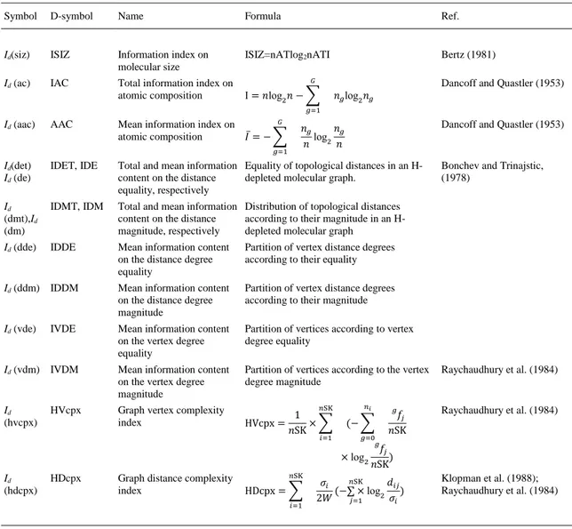
(9) The total information content of a system having n elements is defined by the following: 𝐺. 𝐼 = 𝑛log 2 𝑛 − ∑. 𝑛𝑔 log 2 𝑛𝑔. 𝑔=1. where G is the number of different equivalence classes and ng is the number of elements in the gth class. Each equivalence class is built by the definition of some relationships among the elements of the system. The logarithm is taken at base 2 for measuring the information content in bits. The total information content represents the residual information contained in the system after G relationships are defined among the n elements ( Todeschini and Consonni, 2000). The mean information content, also called Shannon’s entropy is defined as (Shannon and Weaver, 1949): 𝐺. 𝐼̅ = − ∑ 𝑔=1. 𝑛𝑔 𝑛𝑔 log 2 𝑛 𝑛. 2.2.2. Box–Jenkins MA operators of molecular information indices for a single molecule The molecular descriptors used were the Id(k) (13 information indices) of each anti-HIV drug forming the cocktail (131,252 anti-HIV cocktails). The Id(k) descriptors were used as input to calculate MA operators of the biomolecular factors for the drugs. Consequently, to calculate the MA biomolecular operators the value of the drugs information indices Id(k) was needed, as well as the average of these indices for all drugs assayed with the same boundary conditions (cj) of a given biomolecular factor. In general, c1, c2, and c3 refer to different sets of these boundary conditions for the same biomolecular factor (type of assay, molecular targets, cellular lines, organisms, experimental measures, etc.) for a single molecule. A diagram with some examples that describes the methodology used to calculate the inputs corresponding to the drugs is shown in Fig. 1. Δ𝐼𝑑 (𝑘, 𝑑𝑐𝑗 ) = 𝐼𝑑 (𝑘) − 〈𝐼𝑑 (𝑘)〉𝑐𝑗 𝑑=𝑛𝑗. 〈𝐼𝑑 (𝑘)〉𝑐𝑗. 1 = ∑ 𝑛𝑗. 𝑑=1. 𝐼𝑑 (𝑘).
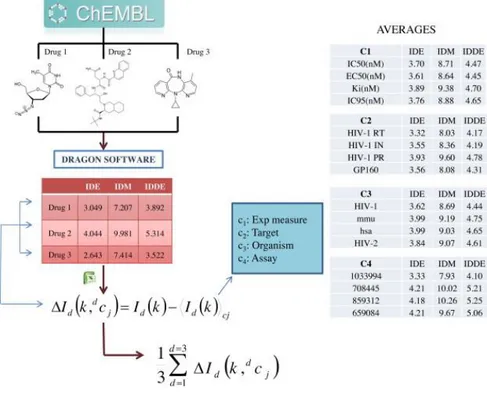
(10) Fig. 1. Calculation details of the inputs of the anti-HIV drugs (left branch of Fig. 2).. 2.2.3. Box–Jenkins MA operators of molecular information indices for HAART drug cocktails In the case of an MA operator for cocktail drugs (up to three molecules in the HAART cocktails studied herein), the MA operators of single drugs were used as input. These MA operators for cocktails take into consideration the sets of conditions dcj = [dc1, dc2, dc3, dc4] for each drug. In general, 1c, 2c, and 3c refer to different sets of these boundary conditions for the same biomolecular factor (type of assay, molecular targets, cellular lines, organisms, experimental measures, etc.). Therefore, 1c1, 2c1,3c1 = are the experimental measures of activity for the first, second, and third drugs of the cocktail, respectively. In analogy, 1c2, 2c2, and 3c2 are the protein targets for the same drugs. In addition, 1c3, 2c3, and 3c3 are the organisms that express the targets of these compounds. Last, 1c4, 2c4, and 3c4 are the different assay protocols used to test the activity of these compounds per se. The MA operator for a drug cocktail was calculated as the arithmetic mean of the corresponding MA operator for each drug in the cocktail. 𝑑=3. Δ𝐼𝑐 (𝑘, 𝑑𝑐𝑗 ) =. 1 ∑ 3. 𝑑=1. 𝑑=3. Δ𝐼𝑑 (𝑘, 𝑐𝑗 ) =. 1 ∑ 3. 𝑑=1. [𝐼𝑑 (𝑘) − 〈𝐼𝑑 (𝑘)〉𝑐 ] 𝑗. The information indices Id(k) of the molecules, the average values <Id(k)>cj of these indices for different boundary conditions (cj), and relevant information for biomolecular factors of all drugs are shown in Tables SM2 and SM3 of Supplementary material, respectively. A diagram summarizing the above steps is depicted in Fig. 2..
(11) Fig. 2. Flowchart used to construct the ANNs for the AIDS Pharmacoepidemiology model in the U.S.. 2.3. ALMA models of complex networks 2.3.1. Linear ALMA models ALMA (assessing links with moving averages) is a technique developed by our group that has been previously used to construct complex multi-scale networks of AIDS and anti-HIV drugs (González-Díaz et al., 2014 and Herrera-Ibatá et al., 2014). In the previous study, MA operators of biomolecular and socioeconomic factors were used. In this work, the ALMA technique was employed to fit a new class of dual models combining chemoinformatics and epidemiological data for HAART cocktails made up of combinations of 1–3 anti-HIV drugs. These new models are able to link AIDS epidemiology data with socioeconomic and population structure data of the U.S. counties and preclinical structure–activity information of all compounds combined in each HAART cocktail. The MA of operators of nodes of networks (drugs, proteins, organisms, populations, etc.) was used to predict the variable Lac(dcj)obs. The value is Lac(cj) = 1 when the cocktail-disease ratio = CDRac(dcj) > cutoff and Laq(dcj)obs = 0 otherwise. The term CDRac(cj) = [zc/Da]; where zc = (z1 + z2 + z3)/3 = the average of the z-scores z1, z2, z3 of the biological activity for each drug (dth) present in the cocktail. The term Da is the AIDS prevalence rate for the ath county. Each zeta was calculated as zd(cj) = δj·zd(cj) = δj· [vd(cj) − AVG(v(cj))]/SD(v(cj)). In this operator, vd(cj) is the value of biological activity (EC50, IC50, Ki, … etc.) reported in the ChEMBL database for the dth drug assayed in the set of conditions. The parameter δj is similar to a Kronecker delta function. The parameter δj = 1 when the biological activity parameter vd(cj) is directly proportional to the biological effect (e.g., Ki values, activity (%) values, etc.). Conversely, δj = −1 when the biological activity parameter vd(cj) is inversely proportional to the biological effect (e.g., EC50 values, IC50 values, etc.). The parameter zd(cj) is the z-score of the biological activity that depends on the AVG and SD functions. These functions are the average and standard deviation of vd(cj) for all drugs assayed in the same conditions. The reader should note that the predicted, output, or dependent variable of an ALMA model is not a discrete variable but a real-valued numerical score (Sac). However, the variable is directly proportional to the observed variable. The general formula for a linear ALMA model developed using average values of ΔIa(L, v) and ΔIc indices of the counties and compounds used in a given drug cocktail was:.
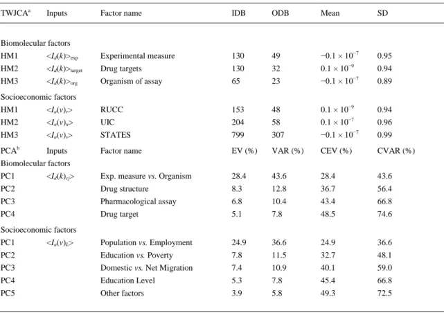
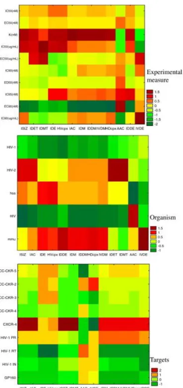
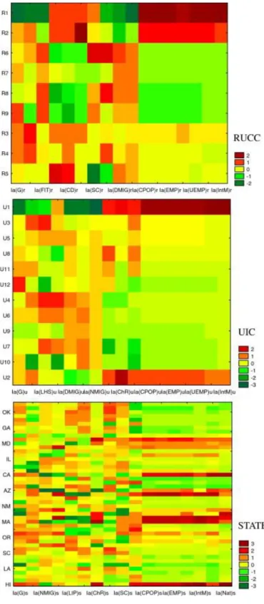
(12) 𝑘=13. 𝑗=4. 𝐿=3 𝑑. 𝑣=17. 𝑆ac = ∑. ∑. 𝑒𝑘𝑗 × Δ𝐼𝑐 (𝑘, 𝑐𝑗 ) + ∑. ∑. 𝑘=1. 𝑗=1. 𝐿=1. 𝑣=1. 𝑒𝐿𝑣 × Δ𝐼𝑎 (𝐿, 𝑣) + 𝑒0. 3. Results and discussion 3.1. Two-way joining cluster analysis and principal components analysis The two-way joining cluster analysis (TWJCA) and principal components analysis (PCA) are useful methods to reduce the magnitude of datasets with many input variables. Two-way joining is useful in circumstances in which it is expected that both cases and variables will simultaneously contribute to find meaningful patterns of clusters (Hill and Lewicki, 2006). A dichotomist approach for both TWJCA and PCA was used herein. It means that TWJCA and PCA of socioeconomic and biomolecular factors were carried out separately. These techniques were used in order to perform a preliminary exploratory study of the data and to determine their variability. In addition, the discriminatory effect of the information indices was studied under the different conditions of assay. First, TWJCA was employed to analyze the biomolecular data. The TWJCA algorithm reorganized the average values of the information indices with respect to those compounds with the same experimental measure, drug targets, and organism of assay into a total number of blocks (see Table 6 and Fig. 3). For example, the experimental measure present an initial input of blocks, 130, resulting in 49 output blocks after performing the TWJCA. As it can be seen in the hot maps (HM) depicted in Fig. 3, the experimental measure and biomolecular targets show that there is no information index that distinguishes well each condition for the experimental measure and targets. However, some indices (IDET, IDMT, and ISIZ) represent clearly the CXCR-4 receptor. Moreover, in the figure corresponding to the organism, the ISIZ index discriminates well each organism of assay (HIV-1, HIV-2, hsa, etc.). Next, TWJCA of the socioeconomic data was performed. In the specific case of TWJCA for socioeconomic data, the analysis of different levels of population distribution (UIC, RUCC and State) was also carried out separately. The HM obtained by cluster analysis does not show significant differences between the metro and nonmetro codes and the population structures (see Fig. 4)..
(13) Table 6. TWJCA and PCA of average values of information indices for drugs <Id(k)>cj and counties <Ia(v)>L. TWJCAa. Inputs. Factor name. IDB. ODB. Mean. SD. Biomolecular factors HM1. <Id(k)>exp. Experimental measure. 130. 49. −0.1 × 10⁻⁷. 0.95. HM2. <Id(k)>target. Drug targets. 130. 32. 0.1 × 10⁻⁹. 0.94. HM3. <Id(k)>org. Organism of assay. 65. 23. −0.1 × 10⁻⁷. 0.89. Socioeconomic factors HM1. <Ia(v)r>. RUCC. 153. 48. 0.1 × 10⁻⁹. 0.94. HM2. <Ia(v)u>. UIC. 204. 58. 0.1 × 10⁻⁷. 0.96. HM3. <Ia(v)s>. STATES. 799. 307. −0.1 × 10⁻⁷. 0.99. Inputs. Factor name. EV (%). VAR (%). CEV (%). CVAR (%). b. PCA. Biomolecular factors PC1. Exp. measure vs. Organism. 28.4. 43.6. 28.4. 43.6. PC2. <Id(k)cj>. Drug structure. 8.3. 12.8. 36.7. 56.4. PC3. Pharmacological assay. 6.8. 10.4. 43.4. 66.8. PC4. Drug target. 5.1. 7.8. 48.5. 74.6. Socioeconomic factors PC1. Population vs. Employment. 24.9. 36.6. 24.9. 36.6. PC2. Education vs. Poverty. 7.8. 11.5. 32.7. 48.1. PC3. Domestic vs. Net Migration. 7.4. 10.9. 40.1. 59.0. PC4. Education Level. 5.3. 7.8. 45.4. 66.8. PC5. Other factors. 3.9. 5.8. 49.3. 72.5. a. <Ia(v)L>. TWJCA = two-way joining cluster analysis; HM = hot maps (Fig. 4 and Fig. 5), IDB = input data blocks, ODB = output data blocks, SD = standard deviation (threshold value = SD/2). b PCA = principal component analysis (Fig. 6), EV = eigenvalue, CEV = cumulative eigenvalues, VAR = variance, CVAR = cumulative variance..
(14) Fig. 3. Hot maps (HM) picture of TWJCA results with average values <Id(k)>cj of the information indices Id(k) for different biomolecular factors (cj)..
(15) Fig. 4. Hot maps (HM) of TWJCA results with average values <Ia(k)>cj of the information indices Ia(k) for different socioeconomic factors structure population (cj = R = RUCC level, U = UIC level, S = State level)..
(16) On the one hand, a PCA of data was carried out. PCA was applied in this work with two different aims. The first was to represent the complex data of anti-HIV drug cocktails vs. U.S. counties in a compact form and analyze the results. The PCA for the socioeconomic factors was performed with 68 input variables, resulting in four factors that represent the 72% of the information (see Table 6). The plot of socioeconomic eigenvalues can be seen in Fig. 5. The first factor represents the population and employment, the second factor shows the information about education and poverty, the third one is the domestic and net migration and the fourth factor refers to education level. On the other hand, the PCA for the biomolecular factors was conducted with 65 input variables. In this case, the analysis showed four eigenvalues for the biomolecular factors that account for the 74% of the information, the first factor being the experimental measure and organism, the second factor the drug structure, the third factor the assay and the fourth factor the target (Fig. 5). Table 6 depicts the eigenvalues obtained for the different principal components. The eigenvalues generated during PCA give an indication of the amount of information carried by each component.. Fig. 5. Plot of biomolecular and socioeconomic eigenvalues for PCA of average values..
(17) 3.2. ANN calculation of parameters in a linear and non-linear ALMA model In our previous work (González-Díaz et al., 2014), a LNN model was developed using Balaban information indices for anti-HIV compounds present in the ChEMBL database (unique drugs = 21,582 and total data points = 43,249). The model also included the Shannon entropy information indices based on values of Gini income inequality of the U.S. counties (Pabayo et al., 2014). The model presented values of accuracy (Ac), specificity (Sp), and sensitivity (Sn) ≈ 0.75 in training and external validation series. In this work, different ANNs were trained using the MA operators for the information indices of several socioeconomic and biomolecular inputs. In total, 40 MA operators were used for the different biomolecular conditions of drugs cocktails (experimental measures, targets and organism) and 50 MA operators of the socioeconomic factors in the U.S. counties. The MA of socioeconomic factors for each county was calculated in the form of deviations from all counties with the same populations, with the same structure (i.e., RUCC or UIC code) or with the same geographic location (same State). Finally, different prediction models were obtained. The dataset used to perform the model includes N = 131,252 statistical cases. The data used to train the model included N = 78,752 statistical cases, selection involved 26,250 statistical cases and validation included 26,250 statistical cases. There were 22,100 cases with Lac(cj)obs = 1 and 109,152 cases with Lac(cj)obs = 0. The ANN module implemented in the STATISTICA 6.0 software package (Hill and Lewicki, 2006) was employed. The statistical parameters used to support the model were: number of cases in training (N), and overall values of specificity (Sp), sensitivity (Sn), accuracy (Ac), and AUROC (area under receiver operating curve). Different topologies of ANNs were trained, including multilayer perceptrons (MLPs) and linear neural networks (LNN). Last, ALMA models using a PCA–ANN approach was also trained. In fact, the output of the PCA can be copied to the dataset, and used to train the ANN with a notably lower number of input variables. An analysis of >130,000 pairs (network links) was carried out, corresponding to AIDS prevalence in 2310 counties in the U.S. vs. drug cocktails made up of combinations of ChEMBL results for 21,582 unique drugs, 9 viral or human protein targets, 4856 protocols, and 10 possible experimental measures. The parameters of the generated ANNs are depicted in Table 7. The best model found with original data was a linear neural network (LNN) with AUROC > 0.80 and Ac, Sp, and Sn ≈ 79% in training and external validation series, and the predictive model presented 87 variables. However, the UIC-LNN model was chosen because its performance is Ac, Sp, and Sn ≈ 77% in training and external validation series using 54 variables (see Table SM4 of Supplementary material, with variables for each model). In addition, the urban influence codes presented a more specific classification scheme for structure population.. Table 7. Parameters of generated ANNs. Population. Net. name. Training algorithm. Error function. Hidden activation. Output activation. All. MLP 90-14-2. BFGS 193. Entropy. Logistic. Softmax. State. MLP 56-23-2. BFGS 68. SOS. Logistic. Logistic. RUCC. MLP 56-15-2. BFGS163. Entropy. Identity. Softmax. UIC. MLP 56-15-2. BFGS140. SOS. Tanh. Identity. Population. Net. name. Training algorithm. Error function. Activation. Hidden layers. All. LNN 87:87-1:1. Pseudoinverse. Entropy. Identity. 0. State. LNN 52:52-1:1. RUCC. LNN 53:53-1:1. UIC. LNN 54:54-1:1. BFGS = Broyden–Fletcher–Goldfarb–Shanno, or Quasi-Newton; SOS = sum of squares..
(18) Furthermore, the population structure scale (State, UIC, or RUCC codes) does not affect the quality of the model (see Table 8). This may indicate that the efficiency of a cocktail from an epidemiological point of view does not depend on the demographic structure of the population. However, the inclusion of different socioeconomic factors seems to affect the accuracy of the model. The SES depends on a combination of variables including occupation, education, income and place of residence, therefore the relationship between the social determinants and AIDS has a significant role to play in the adherence to HAART therapy (Falagas et al., 2008). Nevertheless, evidence of the association between adherence to HIV therapy and socioeconomic status is still rudimentary, varied and there is no a conclusive support for the existence of a clear association. Some studies found lower socioeconomic status (SES) to be associated with higher mortality from AIDS (McFarland et al., 2003). Recent evidence indicates that AIDS is a disease of inequality, often associated with economic transition, rather than a disease of poverty in itself (Piot et al., 2007). Additionally, many researchers now point not to poverty itself but to economic and gender inequalities and weakened “social cohesion” (Barnett and Whiteside, 2006) as factors influencing sexual behavior and hence the potential for HIV transmission. Undeniably, more people live with HIV in poor countries than in rich ones. More than 60% of people living with HIV inhabit the world's poorest region: sub-Saharan Africa. However, studies during the early stage of the epidemic suggested that HIV incidence initially occurred not amongst the poorest, but among better-off members of society in this region. A decade later, infections still appear more concentrated among the urban employed and more mobile members of society, and consequently the more wealthy groups (Piot et al., 2007).. Table 8. ALMA models based on ANN classifiers found with STATISTICA using original data. Level. ANN models. State. Training Observed. MLP 56-23-2 Parametera. LNN 52:521:1. RUCC. UIC. Lac = 1. Lac = 0. Lac = 1. Lac = 0. Lac = 1. Lac = 0. Sn. Sp. Sn. Sp. Sn. Sp. 16.58. 98.20. 10.98. 98.42. 12.84. 97.48. Lac = 1. 2189. 1177. 503. 342. 556. 551. Lac = 0. 11006. 64380. 4074. 21331. 3772. 21371. Parametera. Sn. Sp. Sn. Sp. Sn. Sp. Predicted. 77.16. 75.32. 73.89. 75.77. 73.23. 76.32. Lac = 1. 10182. 16174. 3198. 5310. 3352. 5131. Lac = 0. 3013. 49383. 1130. 16612. 1225. 16542. Observed. Lac = 1. Lac = 0. Lac = 1. Lac = 0. Lac = 1. Lac = 0. Sn. Sp. Sn. Sp. Sn. Sp. Predicted. 31. 96. 28. 96. 30. 96. Lac = 1. 4213. 2281. 1320. 681. 1329. 770. Lac = 0. 8982. 63276. 3257. 20992. 2999. 21152. Parametera. Sn. Sp. Sn. Sp. Sn. Sp. Predicted. 79.37. 77.07. 76.38. 77.38. 73.30. 79.22. Lac = 1. 10473. 15031. 3306. 4957. 3355. 4502. Lac = 0. 2722. 50526. 1022. 16965. 1222. 17171. Observed. Lac = 1. Lac = 0. Lac = 1. Lac = 0. Lac = 1. Lac = 0. Sn. Sp. Sn. Sp. Sn. Sp. Predicted. 34.99. 97.15. 26.69. 96.89. 28.14. 97.13. Lac = 1. 4618. 1865. 1222. 674. 1218. 627. Lac = 0. 8577. 63692. 3355. 20999. 3110. 21295. Parametera. Sn. Sp. Sn. Sp. Sn. Sp. Predicted. 79.67. 77.07. 76.73. 77.52. 72.97. 79.03. Lac = 1. 10513. 15027. 3321. 4926. 3340. 4544. MLP 56-15-2 Parametera. LNN 54:541:1. Validation. Predicted. MLP 56-15-2 Parametera. LNN 53:531:1. Selection.
(19) Table 8. ALMA models based on ANN classifiers found with STATISTICA using original data. Level. ANN models. State. ALL. Training. PCA. Lac = 1. Lac = 0. Lac = 1. Lac = 0. Lac = 1. Lac = 0. Lac = 0. 2682. 50530. 1007. 16996. 1237. 17129. Observed. Lac = 1. Lac = 0. Lac = 1. Lac = 0. Lac = 1. Lac = 0. Sn. Sp. Sn. Sp. Sn. Sp. Predicted. 58.55. 96.18. 49.09. 94.80. 48.93. 94.32. Lac = 1. 7726. 2498. 2247. 1125. 2118. 1243. Lac = 0. 5469. 63059. 2330. 20548. 2210. 20679. Parametera. Sn. Sp. Sn. Sp. Sn. Sp. Predicted. 80.93. 79.83. 80.26. 80.31. 77.14. 80.99. Lac = 1. 10680. 13221. 3474. 4316. 3531. 4118. Lac = 0. 2515. 52336. 854. 17606. 1046. 17555. Observed. Lac = 1. Lac = 0. Lac = 1. Lac = 0. Lac = 1. Lac = 0. Sn. Sp. Sn. Sp. Sn. Sp. Predicted. 61.42. 57.07. 52.86. 60.55. 53.68. 57.95. Lac = 1. 8104. 28146. 2288. 8649. 2457. 9113. Lac = 0. 5091. 37411. 2040. 13273. 2120. 12560. Parametera. Sn. Sp. Sn. Sp. Sn. Sp. Predicted. 58.54. 56.84. 51.15. 58.46. 55.25. 52.34. Lac = 1. 7725. 28295. 2214. 9107. 2529. 10330. Lac = 0. 5470. 37262. 2114. 12815. 2048. 11343. MLP 6:6-8-1:1 Parametera. LNN 7:7-1:1. a. Validation. Observed. MLP 90-14-2 Parametera. LNN 87:871:1. Selection. Parameters, Sp = specificity, Sn = sensitivity; columns: observed classifications; rows: predicted classifications. Training ALMA models using PCA–ANN fails to generate good predictions classifiers, with Sp and Sn results close to 50% in MLP and LNN networks (see Table 8). In this work, the UIC–LNN model was chosen, because it is a more specific classification scheme of the population structure than the others and LNN is the simplest type of classification model. The UIC–LNN model shows values of AUROC = 0.85 in training and AUROC = 0.83 for the external validation set (see Fig. 6)..
(20) Fig. 6. ROC for ALMA–LNN model with MA of socioeconomic factors related to the UIC codes.. However, certain unbalance was noted regarding the classification of positive/negatives cases, as well as on the predictive power of linear vs. non-linear classifiers. Using SMOTE data pre-processing and machine-learning algorithms implemented in the WEKA software (Hall et al., 2009), more balanced models were found. In particular, as it can be seen in Table 9, an MLP with AUROC = 97.4% and precision, recall, and F-measure >90% was found. First, a hybrid preprocessing approach called SMOTE (Chawla et al., 2002) was used, based on oversampling and undersampling our highly imbalanced dataset in order to equilibrate the two output classes. This generates a substantial improvement of results on the test set implemented into the non-linear models, the increase in precision or positive predictive value given being of particular importance, which is the main goal of our research. The MLP and random forest methods are applied, as they are more computationally demanding schemes, able to uncover underlying complex and non-linear functions between the variables. In conclusion, our data seem to be better modelled through a combination of previous preprocessing and the application of non-linear machine learning algorithms, as reflected in Table 9..
(21) Table 9. Results for models obtained with WEKA before and after obtaining the SMOTED data. WEKA modelsa. Parameters. Original datab. Precision. Recall. F-measure. AUROC. VP. 19.5. 33.6. 24.6. 52.9. MLP. 59.3. 57.3. 58.3. 86.2. RNDF. 60.3. 43.3. 50.4. 82.1. SMOTE data filter. c. Precision. Recall. F-measure. AUROC. VP. 50.1. 74.9. 60.0. 49.9. MLP. 94.2. 90.1. 92.1. 97.4. RNDF. 91.7. 89.4. 90.5. 95.9. a. VP = voted perceptron, MLP = multi-layer perceptron, RNDF = random forest. Models obtained with WEKA prior to data pre-processing. c Models obtained with WEKA using SMOTED data. b. 3.3. Back-projection of the computational chemistry model over U.S. county sub-networks The output values (Lac(dcj)obs = 1 or Lac(dcj)obs = 0) of the ALMA classifier were used to generate different sub-networks. This variable quantifies the formation of links between nodes in the core complex network. This network maps the AIDS prevalence with respect to the preclinical activity of anti-HIV drug cocktails in each state of the U.S. at county level. This network has two parts, the core and the periphery. There are two different types of nodes making up the core of this specific network. The first type represents the U.S. counties (ath) and the second type of nodes represents the HAART cocktails (cth). In addition, each cocktail node has 2–3 nodes attached to it, which represents the drugs present in the cocktail (network periphery). Fig. 7 shows a sub-network (of the previous type of network) for AIDS prevalence in the state of New York (NY) vs. anti-HIV drug preclinical activity for all drugs combined in the HAART cocktails designed from compounds reported in ChEMBL. The sub-network contains three types of nodes; the nodes of the network core are the US counties (red) and the HAART cocktails (blue). The nodes of the periphery of the network are anti-HIV compounds combined to making up different cocktails (nodes hidden in the picture). It is important to understand that here Lac(cj)pred = 1 expresses the existence of a sub-graph that connects several nodes of all classes by means of various arcs and no single arcs connecting two nodes. It is possible to create a similar type of sub-network with a model reported in a previous work (Herrera-Ibatá et al., 2014). In the mentioned study, the type of sub-network may have different classes of nodes. There are three main classes: the counties of the state, the drug cocktails, and the chemical compounds making up the cocktail. However, this sub-network includes only one socioeconomic variable: the Gini coefficient. Furthermore, another type of sub-network was developed in a previous work (González-Díaz et al., 2014), which had two classes of nodes (counties vs. drugs). The drug nodes contained information about the chemical structure, as well as all the assay conditions (target, organism, assay protocol, experimental measure). Additionally, the county nodes contained the information about the income inequality. However, because of the type of model used, those complex networks are unable to represent drug cocktails..
(22) Fig. 7. Predicted sub-network of HAART cocktails vs. AIDS prevalence for the state of New York (NY).. 3.4. Computational chemistry modeling of AIDS epidemiology in the U.S. counties network The probabilities with which AIDS could be halted using several drug cocktails in a given county (ath) were calculated. It is important to explain that not all counties were modelled against every drug cocktail. 𝑝𝑎 (halt) =. 𝛿in (𝑎)NY 𝑛(𝐿ac = 1) = 𝑓(𝑎)NY 𝑓(𝑎)NY. In the example with the state of New York, the symbol δin(a)NY = n(Lac = 1) is the number (n) of cocktails predicted to be effective to halt the AIDS outbreak in the ath county. The county in-degree is the number of links (Lac(cj)pred = 1) between the different cocktails and the county. The county frequency refers to the total number of times that the county is in our database. Moreover, Table 10 depicts some examples from the complex sub-network of the state of New York, with data of counties in-degree with several HAART cocktails. For example, Bronx County shows a good in-degree in the complex subnetwork, e.g., the probability that several HAART cocktails are effective in this county is higher than in Chemung county, which presents a lower probability. Thus, this type of model could be useful for epidemiological surveillance procedures to understand the vulnerability of the populations regarding AIDS epidemic..
(23) Table 10. Predicted probabilities, p (halt), with which AIDS could be halted in a county with a HAART cocktail. NY County. County frequency. County in-degree. p (halt). Bronx. 57. 48. 0.84. Queens. 57. 43. 0.75. New York. 56. 41. 0.73. Kings. 56. 39. 0.70. Westchester. 57. 30. 0.53. Jefferson. 56. 18. 0.32. Orange. 56. 17. 0.29. Rockland. 56. 16. 0.29. Dutchess. 57. 16. 0.28. Chemung. 57. 14. 0.25. 4. Conclusions ALMA models were used to carry out a back-projection of the preclinical activity of drugs combined in a HAART cocktail over a complex network of AIDS in the U.S. counties. In this work, the UIC–LNN model was chosen, because it is a more specific classification scheme of the population structure than the other ones and LNN is the simplest type of classification model. However, an unbalance was noted regarding the classification of positive/negatives cases, as well as regarding the predictive power of linear vs. non-linear classifiers. In consequence, our dataset was transformed with data pre-processing algorithms and three different machine-learning algorithms implemented in the WEKA software ( Hall et al., 2009). First, a hybrid preprocessing approach called SMOTE (Chawla et al., 2002) was used. This generates a substantial improvement of results on the test set implemented into the non-linear models. More balanced models were found, such as an MLP with AUROC = 97.4%, precision, recall, and Fmeasure >90%. The generated models based on machine-learning algorithms (ANNs mainly) could be useful as an initial form of screening for the prediction of effective drugs in preclinical assays for the treatment of HIV in different populations of U.S. counties with a given AIDS epidemiological prevalence. Thus, this is cost and time effective, compared to the expensive process of drug discovery and development. The artificial intelligence techniques and procedures employed do not prove a definite relationship between adherence to HIV treatment and socioeconomic status, since this is still rudimentary and there is no strong support for the existence of a clear association.. Acknowledgements R.O.M acknowledges financial support of FPI fellowship funded by MECD (Ministry of Education, Culture and Sport, Spain).. References Internal Revenue Service, 2014. Internal Revenue Service (February, 2014). Tax Foundation, http://taxfoundation.org/resources. Aguilera and Rodriguez-Gonzalez, 2014. L.U. Aguilera, J. Rodriguez-Gonzalez. Studying HIV latency by modeling the interaction between HIV proteins and the innate immune response. J. Theor. Biol., 360 (2014), pp. 67–77 http://dx.doi.org/10.1016/j.jtbi.2014.06.025. Barnett and Whiteside, 2006. T. Barnett, A. Whiteside. AIDS in the Twenty-first Century: Disease and Globalization. Palgrave Macmillan, New York (2006). Barresi et al., 2013. V. Barresi, C. Bonaccorso, G. Consiglio, L. Goracci, N. Musso, G. Musumarra, C. Satriano, C.G. Fortuna. Modeling, design and synthesis of new heteroaryl ethylenes active against the MCF-7 breast cancer cellline. Mol. Biosyst., 9 (2013), pp. 2426–2429 http://dx.doi.org/10.1039/c3mb70151d..
(24) Bento et al., 2013. A.P. Bento, A. Gaulton, A. Hersey, L.J. Bellis, J. Chambers, M. Davies, F.A. Kruger, Y. Light, L. Mak, S. McGlinchey, M. Nowotka, G. Papadatos, R. Santos, J.P. Overington. The ChEMBL bioactivity database: an update. Nucleic Acids Res., 42 (2013) http://dx.doi.org/10.1093/nar/gkt1031. Bertz, 1981. S.H. Bertz. The first general index of molecular complexity. J. Am. Chem. Soc., 103 (1981), pp. 3599– 3601. Bonchev and Trinajstic, 1978. D. Bonchev, N. Trinajstic. On topological characterization of molecular branching. Int. J. Quantum Chem. Quant. Chem. Symp., 12 (1978), pp. 293–303. Brown et al., 1976. D.L. Brown, F.K. Hines, J.M. Zimmer. Social and Economic Characteristics of the Population in Metro and Nonmetro Counties: 1970. Economic Research Service, U.S. Deptrtment of Agriculture (1976) AER272. Burbidge et al., 2001. R. Burbidge, M. Trotter, B. Buxton, S. Holden. Drug design by machine learning: support vector machines for pharmaceutical data analysis. Comput. Chem., 26 (2001), pp. 5–14. Castilla et al., 2005. J. Castilla, J. Del Romero, V. Hernando, B. Marincovich, S. Garcia, C. Rodriguez. Effectiveness of highly active antiretroviral therapy in reducing heterosexual transmission of HIV. J. Acquir. Immune Defic. Syndr., 40 (2005), pp. 96–101. CDC, 2013. CDC. HIV infection among heterosexuals at increased risk – United States, 2010. MMWR Morb. Mortal Wkly. Rep., 62 (2013), pp. 183–188. Colombo et al., 2014. G.L. Colombo, A. Castagna, S. Di Matteo, L. Galli, G. Bruno, A. Poli, S. Salpietro, A. Carbone, A. Lazzarin. Cost analysis of initial highly active antiretroviral therapy regimens for managing human immunodeficiency virus-infected patients according to clinical practice in a hospital setting. Ther. Clin. Risk Manage., 10 (2014), pp. 9–15 http://dx.doi.org/10.2147/tcrm.s49428. Chawla et al., 2002. N.V. Chawla, K.W. Bowyer, L.O. Hall, W.P. Kegelmeyer. SMOTE: synthetic minority oversampling technique. J. Artif. Int. Res., 16 (2002), pp. 321–357. Dancoff and Quastler, 1953. S.M. Dancoff, H. Quastler. Essays on the Use of Information Theory in Biology. University of Illinois, Urbana (1953). Falagas et al., 2008. M.E. Falagas, E.A. Zarkadoulia, P.A. Pliatsika, G. Panos. Socioeconomic status (SES) as a determinant of adherence to treatment in HIV infected patients: a systematic review of the literature. Retrovirology, 5 (2008). Gaulton et al., 2012. A. Gaulton, L.J. Bellis, A.P. Bento, J. Chambers, M. Davies, A. Hersey, Y. Light, S. McGlinchey, D. Michalovich, B. Al-Lazikani, J.P. Overington. ChEMBL: a large-scale bioactivity database for drug discovery. Nucleic Acids Res., 40 (2012), pp. D1100–D1107 http://dx.doi.org/10.1093/nar/gkr777. Ghelfi and Parker, 1997. L.M. Ghelfi, T.S. Parker. A county-level measure of urban influence. Rural Dev. Perspect., 12 (1997). Gonzalez-Diaz et al., 2011. H. Gonzalez-Diaz, F. Prado-Prado, E. Sobarzo-Sanchez, M. Haddad, S. Maurel Chevalley, A. Valentin, J. Quetin-Leclercq, M.A. Dea-Ayuela, M. Teresa Gomez-Munos, C.R. Munteanu, J. Jose Torres-Labandeira, X. Garcia-Mera, R.A. Tapia, F.M. Ubeira. NL MIND-BEST: a web server for ligands and proteins discovery – theoretic-experimental study of proteins of Giardia lamblia and new compounds active against Plasmodium falciparum. J. Theor. Biol., 276 (2011), pp. 229–249 http://dx.doi.org/10.1016/j.jtbi.2011.01.010. González-Díaz et al., 2014. H. González-Díaz, D.M. Herrera-Ibatá, A. Duardo-Sanchez, C.R. Munteanu, R.A. Orbegozo-Medina, A. Pazos. Model of the multiscale complex network of AIDS prevalence in US at county level vs. preclinical activity of anti-HIV drugs based on information indices of molecular graphs and social networks. J. Chem. Inf. Model, 54 (2014), pp. 744–755. Guha, 2013. R. Guha. On exploring structure-activity relationships. Methods Mol. Biol., 993 (2013), pp. 81–94 http://dx.doi.org/10.1007/978-1-62703-342-8_6. Hall et al., 2009. M. Hall, E. Frank, G. Holmes, B. Pfahringer, P. Reutemann, I.H. Witten. The WEKA data mining software: an update. SIGKDD Explor. Newslett., 11 (2009), pp. 10–18 http://dx.doi.org/10.1145/1656274.1656278. Heikamp and Bajorath, 2011. K. Heikamp, J. Bajorath. 2011: Large-scale similarity search profiling of ChEMBL compound data sets. J. Chem. Inf. Model., 51 (2011), pp. 1831–1839 http://dx.doi.org/10.1021/ci200199u. Herrera-Ibatá et al., 2014. D.M. Herrera-Ibatá, A. Pazos, R.A. Orbegozo-Medina, H. Gonzalez-Diaz. Mapping networks of anti-HIV drug cocktails vs: AIDS epidemiology in the US counties. Chemometr. Intell. Lab., 138 (2014), pp. 161–170. Hill and Lewicki, 2006. T. Hill, P. Lewicki. STATISTICS methods and applications. A Comprehensive Reference for Science, Industry and Data Mining, StatSoft, Tulsa, Oklahoma (2006). Holtgrave and Crosby, 2003. D.R. Holtgrave, R.A. Crosby. Social capital, poverty, and income inequality as predictors of gonorrhoea, syphilis, chlamydia and AIDS case rates in the United States. Sex. Transm. Infect., 79 (2003), pp. 62–64. Jain Pancholi et al., 2014. N. Jain Pancholi, S. Gupta, N. Sapre, N.S. Sapre. Design of novel leads: ligand based computational modeling studies on non-nucleoside reverse transcriptase inhibitors (NNRTIs) of HIV-1. Mol. Biosyst., 10 (2014), pp. 313–325 http://dx.doi.org/10.1039/c3mb70218a. Klopman et al., 1988. G. Klopman, C. Raychaudhury, R.V. Henderson. A new approach to structure-activity using distance information content of graph vertices: a study with phenylalkylamines. Math. Comput. Model., 11 (1988), pp. 635–640. McDavid Harrison et al., 2008. K. McDavid Harrison, Q. Ling, R. Song, H.I. Hall. County-level socioeconomic status and survival after HIV diagnosis, United States. Ann. Epidemiol., 18 (2008), pp. 919–927 http://dx.doi.org/10.1016/j.annepidem.2008.09.003..
(25) McFarland et al., 2003. W. McFarland, S. Chen, L. Hsu, S. Schwarcz, M. Katz. Low socioeconomic status is associated with a higher rate of death in the era of highly active antiretroviral therapy, San Francisco. J. Acquir. Immune Defic. Syndr., 33 (2003), pp. 96–103. McMahon et al., 2011. J. McMahon, C. Wanke, N. Terrin, S. Skinner, T. Knox. Poverty, hunger, education, and residential status impact survival in HIV. AIDS Behav., 15 (2011), pp. 1503–1511 http://dx.doi.org/10.1007/s10461-010-9759-z. Mondal and Shitan, 2013. M.N. Mondal, M. Shitan. Relative importance of demographic, socioeconomic and health factors on life expectancy in low- and lower-middle-income countries. J. Epidemiol., 24 (2013), pp. 117–124. Munteanu et al., 2009. C.R. Munteanu, A.L. Magalhaes, E. Uriarte, H. Gonzalez-Diaz. Multi-target QPDR classification model for human breast and colon cancer-related proteins using star graph topological indices. J. Theor. Biol., 257 (2009), pp. 303–311 http://dx.doi.org/10.1016/j.jtbi.2008.11.017. Ogul, 2009. H. Ogul. Variable context Markov chains for HIV protease cleavage site prediction. Biosystems, 96 (2009), pp. 246–250 http://dx.doi.org/10.1016/j.biosystems.2009.03.001. Pabayo et al., 2014. R. Pabayo, I. Kawachi, S.E. Gilman. Income inequality among American states and the incidence of major depression. J. Epidemiol Community Health, 68 (2014), pp. 110–115 http://dx.doi.org/10.1136/jech2013-203093. Patel, 2013. J. Patel. Science of the science: drug discovery and artificial neural networks. Curr. Drug Discov. Technol., 10 (2013), pp. 2–7. Ping et al., 2013. L.H. Ping, C.B. Jabara, A.G. Rodrigo, S.E. Hudelson, E. Piwowar-Manning, L. Wang, S.H. Eshleman, M.S. Cohen, R. Swanstrom. HIV-1 transmission during early antiretroviral therapy: evaluation of two HIV-1 transmission events in the HPTN 052 prevention study. PLoS One, 8 (2013), p. e71557 http://dx.doi.org/10.1371/journal.pone.0071557. Piot et al., 2007. P. Piot, R. Greener, S. Russell. Squaring the circle: AIDS, poverty, and human development. PLoS Med., 4 (2007), pp. 1571–1575 http://dx.doi.org/10.1371/journal.pmed.0040314. Raychaudhury et al., 1984. C. Raychaudhury, S.K. Ray, J.J. Ghosh, A.B. Roy, S.C. Basak. Discrimination of isomeric structures using information theoretic topological indices. J. Comput. Chem., 5 (1984), pp. 581–588. Shannon and Weaver, 1949. C. Shannon, W. Weaver. The Mathematical Theory of Communication. University of Illinois Press, Urbana, United States (1949). Speck-Planche et al., 2012. A. Speck-Planche, V.V. Kleandrova, F. Luan, M.N. Cordeiro. A ligand-based approach for the in silico discovery of multi-target inhibitors for proteins associated with HIV infection. Mol. Biosyst., 8 (2012), pp. 2188–2196 http://dx.doi.org/10.1039/c2mb25093d. Todeschini and Consonni, 2000. R. Todeschini, V. Consonni. Handbook of Molecular Descriptors. Wiley-VCH Verlag GmbH, Weinheim, Germany (2000). Usach et al., 2013. I. Usach, V. Melis, J.E. Peris. Non-nucleoside reverse transcriptase inhibitors: a review on pharmacokinetics, pharmacodynamics, safety and tolerability. J. Int. AIDS Soc., 16 (2013), pp. 1–14 http://dx.doi.org/10.7448/ias.16.1.18567. Weekes and Fogel, 2003. D. Weekes, G.B. Fogel. Evolutionary optimization, backpropagation, and data preparation issues in QSAR modeling of HIV inhibition by HEPT derivatives. Biosystems, 72 (2003), pp. 149–158. Xu et al., 2013. L. Xu, Y. Li, H. Sun, D. Li, T. Hou. Structural basis of the interactions between CXCR4 and CXCL12/SDF-1 revealed by theoretical approaches. Mol. Biosyst., 9 (2013), pp. 2107–2117 http://dx.doi.org/10.1039/c3mb70120d..
(26)
Figure
+7
Documento similar
Our results here also indicate that the orders of integration are higher than 1 but smaller than 2 and thus, the standard approach of taking first differences does not lead to
The draft amendments do not operate any more a distinction between different states of emergency; they repeal articles 120, 121and 122 and make it possible for the President to
In this thesis we have presented several modelling techniques that can improve the cur- rent state-of-art of statistical cosmology: an improved halo modelling, a more realistic
As a result of the ordering strategy we expect the values of Bias(u) and V ar(u) (the average bias and variance of a regressor in an ordered subensemble of size u) to be lower than
reliable for predicting the risk of falling or for discriminating between population groups with different age, illness or level of physical activity 17,18. The identification
Firstly, the exogenous spatial factors show that local governments are influenced by the characteristics of their neighbours (population structure, economic level, etc.). Secondly,
No obstante, como esta enfermedad afecta a cada persona de manera diferente, no todas las opciones de cuidado y tratamiento pueden ser apropiadas para cada individuo.. La forma
Clearly, sampling the source at the start of every slot allows us to detect each and every transition of the DTMC. Instead, our aim here is to use a lower sampling frequency.
