Wage dispersion and trade in Argentina, 1974 1994
18
0
0
Texto completo
(2) WAGE DISPERSION AND TRADE IN ARGENTINA. Second, we regress the imputed demand shift time-series, from Section III, onto trade flows and imported-capital-stock to GDP ratios, and GDP growth rates, we find that manufactured exports appear to rise relative demand and changes in imported-capital-stock have large, statistically significant and positive effects upon relative demand. Section V concludes. I. TRADE REGIME IN ARGENTINA From Protectionism and Democracy to Liberalism and Military Power Between early fifties and 1976, Argentina continued a strategy of Import Substitution Industrialization (ISI), endeavoring to deepen the industrialization process already well underway. High levels of protection, foreign direct investment, and strong industrial growth characterized this period. In 1976 a military government seized power. The new government adopted a neo-liberal market-oriented approach, ending Argentina's long period of ISI based economic policy. The economic authority implemented a program to reduce the size of the government, eliminate subsidies, and deregulate markets -including deregulation of interest rates, capital flows and a reduction of tariffs from an average of about 70 percent to 40 percent. Even justified in its own terms, this economic program responded to the political project adopted by the military government as a long run solution for the situation of social crisis of the mid seventies. The diagnostic was that the roots of the crisis were in the structure of social and institutional relationships. Therefore, the main objective of the military government was to change this structure through social discipline. In particular, to discipline the labor force. The economic program was elaborated attending to this political project, in the notion that an economic system of open market is a necessary condition for the existence of a disciplined society (see Canitrot, 1981). The strategy adopted by the economic authority to establish an open market economy was to reduce import tariffs and to reduce the exchange rate. During the period March 1976 to May 1978, the main economic instrument was the reduction of import tariffs on industrial goods competing with national production. Tariff structure in 1976 was similar to that in 1970. Levels of protection ranked from intermediate goods to capital goods. There was discrimination against imports of goods competing with local production, in particular with consumer goods. Highest tariffs corresponded to textile, iron and steel products. In November 1976 a gradual tariff reduction began. For industrial goods, excluding those with tariffs lower than 25% before 1976, the average tariff went from 94% in 1976 to 35% in 1981 (see Canitrot, 1981). The initial outcome of these policies in 1976-1978 was an increase in durable and capital goods production and investment, and a regressive impact on wages and incomes. After May 1978, import tariffs reduction continued, but this reduction was not as important as the progressive revaluation of the local currency. This revaluation process extended from May 1978 to December 1980. By the end of 1978, Argentina adopted a monetarist approach to the balance of payments, intending to set domestic inflation equal to international inflation, with a pre-announced devaluation schedule. However, domestic inflation did not converge to the international rate, and domestic interest rates continued to increase, due to uncertainty and high costs of financial intermediation. The more lasting outcome of these policies was significant overvaluation of the currency. This led to heavy competition from imports and stagnation of exports. The current account was balanced only through strong inflows of foreign capital, in response to high real domestic interest rates, and through international borrowing. Imports surged, lowering the demand for domestic goods; the low exchange rate reduced the incentives to export; and high domestic interest rates lowered investment. The result was a profound crisis for the industrial sector. In 1981, as a consequence of this crisis in the manufacturing sector, there was a change of president in the military council leading the country, and there was a complete change of the cabinet. In this period the private foreign debt was nationalized. Balance of payments pressures, in large part due to debt service requirements, led to a rise in tariffs to pre-1978 levels. Over the period 1976-1981 the industrial output fell 20%, and industry's share of GDP fell from 28 to 23%. Twenty percent of the largest firms closed, and investment in capital goods fell at 5% per annum. Furthermore the share of salaries in national income fell from 49% to 32.5%. The depth of this crisis and the defeat in the Malvinas war with England ushered in the current period of democracy, with Raul Alfonsin elected President in 1983. Economic Policy and Performance In Re-Democratized Argentina By the time when Alfonsin was elected President, the economic situation was chaotic. Fiscal deficit and money supply were beyond any control. The monthly inflation rate was around 18%. The country was facing a huge external debt -51.8 billion dollars of 1987and the negotiations with foreign lenders were suspended. Despite the attempts made by the democratic government, most of the Page 2.
(3) WAGE DISPERSION AND TRADE IN ARGENTINA. 1980's were characterized by stagnation, fiscal deficit and high, accelerating inflation. GNP stagnated near the 1974 level, and while the population grew 25%, employment grew only 19%. Annual inflation was above 100% for nearly all years, from 1975 through 1990, peaking at 5000% in 1989. In this context, the democratic government introduced modest trade liberalization. Between 1982 and 1984 trade policy was dominated by urgencies due to the adjustment to a new situation characterized by external overindebtedness. The need to generate, fast enough, large fiscal and trade surplus -to attend debt services requirements- worsened the macroeconomic instability. The government increased import tariffs and traditional export taxes, and reduced the refund of non-traditional export taxes. After 1984, in a context characterized by a lower degree of instability and by the pressure conducted by multilateral credit agencies under the "Plan Baker", the government began a gradual trade liberalization program. Trade policy in this period was developed to obtain two goals: first, damping the anti-export bias of the incentives regime; and second, rationalization of the structure of protection for local production. To reduce the anti-export bias of the trade policy, the democratic administration adopted the following measures: a) elimination of export taxes, b) introduction of a regime to refunding manufacturing export taxes; and c) re-establishment of the inputs temporarily admitted regime for the production of 7370 industrial products (see Damill and Keifman, 1992). The measures adopted to rationalize the structure of protection were twofold: a) reduction of the universe of imports subject to quantitative limitations; and b) reduction of tariffs and reduction of the variance between tariffs. In the case of petrochemistry and iron and steel industries, the elimination of quantitative import limitations was complemented by a reduction of tariffs. The tariff reform reduced the levels of protection from a range of 15-53% to a range of 5-40%. The average tariff went from 43% to 30%. However, the tariff on the car industry was maintained at more than 40%. In 1989, a new democratic government began a significant trade reform. Trade policy beginning in 1989 was developed in a very different macroeconomic context, affecting the nature of the policy measures adopted. Two hyperinflationary episodes, one in February 1989 and the other at the beginning of 1990 compel the government to maintain a more restrictive fiscal policy. The process of reduction of quantitative import limitations was completed, with these restrictions eliminated by the end of 1990. There were further reductions in tariffs reaching an structure of three levels by the end of 1991: 0% for raw materials and food products, 11% for inputs and 22% for final goods. The special regime for the car industry was maintained with a tariff of 35%. The average weighted tariff for industrial production fell from 30% in 1988 to 10% in 1991. To reduce tariff dispersion and lower average tariffs, in 1990 the tariffs on specific imports, such as chemicals and food, were reduced to between 20 and 50%. This was followed, in October 1992, by a more substantive trade reform. This included lowering the tariff ceiling to 20%, reducing the tariff floor to zero, with a resulting average tariff of 10%. Further, the surcharge was lowered from 15 to 10%. This process of trade liberalization beginning in 1989 was accompanied by an appreciation of the local currency. As a part of a stabilization program a constitutional amendment was passed linking the new peso one-to-one to the U.S. dollar, the Law of Convertibility. Imposing fiscal balance and pegging the exchange rate to the dollar successfully addressed both the structural and inertial sources of inflation. Inflation fell from a monthly rate of 38.6% in 1989 to a 0.3% (or 3.7% annual) in 1994. While Argentina's post-1990 policies successfully ended inflation and attracted net financial inflows, its exchange rate policy has not been costless. As seen in Figure 1 below, the 100% appreciation of the real exchange rate between 1989 and 1991 had predictable effects on trade. Exports levels have not grown since 1990. Meanwhile, imports - especially of consumption and capital goods - have risen rapidly, leading to a widening trade deficit from mid-1991 onwards. Despite stagnant exports, after zero GDP growth in 1990, GDP growth surged ahead to 8.9% in 1991, 8.7% in 1992 and 6% in 1993. This growth was permitted, mainly, by large net financial inflows. However, in 1994 this pattern changed, with net capital inflows falling from 4.7 billion dollars in the second half of 1993, to 2.5 billion dollars in the first half of 1994. Meanwhile, unemployment has grown steadily, rising from 6% to 9% in 1993 and to 10% at the end of 1994. The Finance Minister has tried to push the unemployment problem aside by arguing that the unemployment is due to an "added worker" effect, of rising labor market participation. However a recent work by Pessino and Giacchino (1994) finds little support for that claim.. II. DATA Page 3.
(4) WAGE DISPERSION AND TRADE IN ARGENTINA. To examine changes in wage dispersion across workers by school groups in Argentina, we use the annual Household Surveys of INDEC (National Statistical Institute) for 1974 through 1994. The surveys provide information on earnings, hours worked, work-place characteristics, education, age, other personal characteristics of individuals and characteristics of their jobs, including employed, self-employed, economic activity of organization, and occupation. III. TIME SERIES ANALYSIS OF RELATIVE WAGES, SUPPLY AND DEMAND RELATIVE WAGES The approach used in this section analyzes the relative wages of more skilled to less skilled workers using detailed demographic cross-classifications of workers by sex, schooling and experience, that imposes little parametric structure upon the data. Following Welch (1979), Murphy and Welch (1991) and Katz and Murphy (1992) (hereafter KM92), we first construct normalized relative wage and relative employment vectors for each year from the cross-sectional household survey data, where the elements of the vectors are demographic cells. For the wage vectors only full-time employees fifteen years or older are used, to maximize comparability of wages across workers and over time. Several variants of the employment vectors are constructed, and used as appropriate; these range from only employees to the total potential labor force (employees, self-employed, unpaid family workers, unemployed workers, discouraged workers, and out-of-labor-force persons). Relative employment matrices are calculated both in hours worked and in numbers of persons, or counts, per cell. The relative employment matrix is the distribution of total hours worked across cells, ni,t . The average of the employment distributions over time, N, is used as constant demographic weight when aggregating across cells. The relative wage matrix, W, is composed of relative wage vectors that are the mean wages per cell divided by a weighted annual average wage, where the weight is the vector N. Thus, for year t we calculate the mean wages per cell and the total hours per cell divided by total annual hours: mw i,t ≡ mean wage for i-th cell and, ni,t ≡ distribution of employment (hours or counts) for the i-th cell. The average distribution of employment over cells for all years, N, is: (1) N ≡ Σt=1T nt/T, where T≡ the total number of years of household surveys Thus, the normalized wage vector for year t, wt, is: (2) wt ≡ mw t / (N´mwt). Page 4.
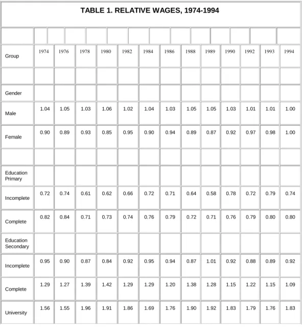
(5) WAGE DISPERSION AND TRADE IN ARGENTINA. For comparisons of relative wages of sub-groups of cells (for example, "university graduates") we typically want comparable price indices unaffected by the changing distributions of workers across cells. To construct such indices, when aggregating wages across cells into larger categories, we use the constant demographic weights, N. For example, if "u" is university education, the fixed-demographic-weighted mean wage for university-educated workers wu, is: (3) wu ≡ Σi∈ u w i ⋅[Ni /Nu], where N u ≡ Σi∈ u N i . This method of aggregation described assures comparability across time, and de-emphasizes outliers for the variables across which we are aggregating. For example, because mean wages for university graduates in year t, or wu,t ( ≡ Σi∈ uw i,t ⋅[Ni /Nu] ), use the average distribution over all years of university educated workers across sex and experience cells, outliers for sex and experience only affect the overall averages, and so have little weight. To aggregate employment across cells of differing productivities, we estimate efficiency units. This is, hours worked in each cell are weighted by the average relative wage of that cell across all years, W. Table 1 presents measures of relative wages for gender and education aggregations. These show that relative wages for workers with some university education fell from 1974 to 1976, rose more than 26% between 1976 and 1978, and then fell steadily until 1984. Then, after increasing from 1984 to 1989, where they reach their highest point, they fell again until 1993, and finally TABLE 1. RELATIVE WAGES, 1974-1994. Group. 1974. 1976. 1978. 1980. 1982. 1984. 1986. 1988. 1989. 1990. 1992. 1993. 1994. 1.04. 1.05. 1.03. 1.06. 1.02. 1.04. 1.03. 1.05. 1.05. 1.03. 1.01. 1.01. 1.00. 0.90. 0.89. 0.93. 0.85. 0.95. 0.90. 0.94. 0.89. 0.87. 0.92. 0.97. 0.98. 1.00. 0.72. 0.74. 0.61. 0.62. 0.66. 0.72. 0.71. 0.64. 0.58. 0.78. 0.72. 0.79. 0.74. 0.82. 0.84. 0.71. 0.73. 0.74. 0.76. 0.79. 0.72. 0.71. 0.76. 0.79. 0.80. 0.80. 0.95. 0.90. 0.87. 0.84. 0.92. 0.95. 0.94. 0.87. 1.01. 0.92. 0.88. 0.89. 0.92. 1.29. 1.27. 1.39. 1.42. 1.29. 1.29. 1.20. 1.38. 1.28. 1.15. 1.22. 1.15. 1.09. 1.56. 1.55. 1.96. 1.91. 1.86. 1.69. 1.76. 1.90. 1.92. 1.83. 1.79. 1.76. 1.83. Gender. Male. Female. Education Primary. Incomplete. Complete. Education Secondary. Incomplete. Complete. University. Page 5.
(6) WAGE DISPERSION AND TRADE IN ARGENTINA. they increase in 1994, reaching in that year the level of 1990. Relative wages for those workers with primary-complete education behave in the opposite direction. They fell after 1976, rose from 1978 to 1986, then fell until 1989 and rose again after that year. This behavior goes against the lines of HOS-X. However, it is consistent with the fact that during the first trade liberalization experiment, the economic program was designed to discipline labor force. Economic measures, like freezing wages and placing worker's unions under government control, probably affected more the wages of workers with lower education than the wages of those with higher education. As a consequence, it is very likely to observe a pattern of relative wages as the one described above. After 1980, the tariff structure reached pre-1978 levels. HOS-X theory would predict an increase in the relative wages of more to less skilled workers. However, they fall until 1984. Therefore, until mid 80s the behavior of relative wages is inconsistent with the HOS-X hypothesis The period, 1986 through 1989, was characterized by high and accelerating inflation, government deficits and mild trade liberalization. Workers with higher education were more fully indexed, so that accelerating inflation would wide wage differentials over most of this. period, as it is shown in Figure 3 (see Menendez, 1996). This effect goes against standard trade theory effects. In 1989, and in early 1990, Argentina faced two hyperinflationary episodes, and relative wages were greatly affected by them. Table 1 and Figure 2 shows the effect of these episodes. Relative wages of more educated workers rose compared with relative wages of less educated workers. This fact is consistent with the idea that more educated people have more instruments to defend their wages from the negative effects of high inflation. Since 1991 on, domestic currency was pegged to the dollar, inflation came to an abrupt stop, economic activity surged and unemployment rose. Also during this period Argentina profounded its trade reform. Summarizing, this period can be characterized as one of trade reform and revaluation. In this scenario, we observe a slight increase in relative wages -measured by the wages of workers with some university education to wages of workers with primary education-. Again, this behavior is not consistent with HOS-X predictions. RELATIVE SUPPLY We next need to create a measure of the relative supply of university graduates to primary school graduates. Because not all workers fall into one of these two categories (for example, some have a secondary education), we create a composite index of relative supply that takes into account information from all workers, using the Linear Skills Synthesis hypothesis of Welch (1969). Welch suggested that while measures of differences in individuals' productive attributes could take on many, even infinite dimensions, skill differences could be characterized in terms of two or three dimensions. Welch characterized these dimensions as physical strength ("brawn") and agility and cognitive ability ("brain"). Individuals would be weighted averages of these two dimensions, and range from mostly Page 6.
(7) WAGE DISPERSION AND TRADE IN ARGENTINA. "brawn" to mostly "brain". We proxy these two dimensions by those with primary-complete education and those with university education -holding other dimensions of skill constant. Workers with either primary complete or university education are allocated entirely to their respective groups. The wages of persons with combinations of the two skill types should be weighted averages of their skill endowments and the returns to those polar skill types. Thus, we regress the time-series of wages of these individuals - say workers with secondary education -onto the time-series of wages of workers with primary-complete and the wages of university educated workers, and construct the weights from the estimated coefficients. We then use these weights to assign workers into the primary or university categories. On this basis workers with secondary education were allocated sixty-eight percent to primary education equivalents, and thirty-two percent to university equivalents. Figure 3 plots relative supply over the entire period. These measures of relative supply rise steadily throughout the 1974-1994 period. These results are robust to different definitions of supply (see Table 2). We focus on the relative supply measure that includes employees, self-employed and unpaid family workers. This measure more than doubles from 1974 to 1994, from 0.21 to 0.52. Since during the first liberalization episode the rise in relative wages occurs concurrent with a continued rise in relative supply, this suggest that relative demand should have shifted towards more skilled workers after trade liberalization. The same occurs between 1986 and 1989 where there is an increase of relative wages and relative supply. This suggest that changes in relative demand were not neutral. We find an increase in the relative supply over the 1985-1994 period, though the increase in the relative supply of workers with some university studies occurs primarily over the 19851989 and over the 1991-1994 periods. In panel 3 of Table 2, we see that the shares of. university educated 26% between 1985 and 1989, only 6% between 1989 and 1991 and 13% between 1991 workers grew and happens with the share of workers with secondary complete education, rising 19% in the 1994. Almost the same 1985-89 interval, 1989-1991only 3% in the TABLE 2. RELATIVE SUPPLY SHARES, 1974-1994. Panel 1. Broad supply measure:employed and self-employed, measured in counts. Page 7.
(8) WAGE DISPERSION AND TRADE IN ARGENTINA. Group. 1974. 1976. 1978. 1980. 1982. 1984. 1986. 1988. 1990. 1993. 1994. 0.68. 0.68. 0.66. 0.67. 0.66. 0.67. 0.63. 0.63. 0.64. 0.62. 0.63. 0.32. 0.32. 0.34. 0.33. 0.34. 0.33. 0.37. 0.37. 0.36. 0.38. 0.37. 0.28. 0.27. 0.25. 0.19. 0.18. 0.16. 0.15. 0.13. 0.10. 0.10. 0.08. 0.35. 0.38. 0.38. 0.36. 0.36. 0.35. 0.32. 0.33. 0.34. 0.30. 0.31. 0.17. 0.16. 0.16. 0.18. 0.19. 0.19. 0.20. 0.20. 0.19. 0.21. 0.19. 0.10. 0.09. 0.11. 0.14. 0.14. 0.15. 0.15. 0.16. 0.17. 0.18. 0.19. 0.09. 0.09. 0.09. 0.14. 0.13. 0.15. 0.17. 0.19. 0.20. 0.21. 0.22. 1974. 1976. 1978. 1980. 1982. 1984. 1986. 1988. 1990. 1993. 1994. 0.67. 0.68. 0.65. 0.67. 0.66. 0.67. 0.62. 0.63. 0.64. 0.62. 0.62. 0.33. 0.32. 0.35. 0.33. 0.34. 0.33. 0.38. 0.37. 0.36. 0.38. 0.38. 0.28. 0.27. 0.25. 0.19. 0.18. 0.16. 0.15. 0.13. 0.10. 0.10. 0.08. 0.35. 0.38. 0.38. 0.36. 0.36. 0.35. 0.32. 0.33. 0.34. 0.30. 0.31. 0.17. 0.16. 0.16. 0.18. 0.19. 0.19. 0.20. 0.20. 0.19. 0.22. 0.21. Gender. Male. Female. Education Primary. Incomplete. Complete. Education Secondary. Incomplete. Complete. University. Panel 2. Labor force. Group. Gender. Male. Female. Education Primary. Incomplete. Complete. Education Secondary. Incomplete. Page 8.
(9) WAGE DISPERSION AND TRADE IN ARGENTINA Incomplete. Complete. University. 0.10. 0.09. 0.11. 0.14. 0.14. 0.15. 0.15. 0.16. 0.17. 0.18. 0.19. 0.09. 0.09. 0.09. 0.13. 0.13. 0.15. 0.17. 0.18. 0.19. 0.21. 0.21. Panel 3. Changes in Relative Supply Group. 74-76. 76-78. 78-83. 83-85. 85-89. 89-91. 91-94. 0.00. -0.03. 0.03. -0.04. -0.01. 0.00. -0.01. -0.01. 0.07. -0.06. 0.09. 0.02. 0.00. 0.02. -0.04. -0.09. -0.41. 0.06. -0.24. -0.17. -0.22. 0.07. 0.01. -0.04. -0.05. -0.10. -0.05. -0.03. -0.03. -0.01. 0.20. -0.01. 0.03. 0.09. -0.02. -0.07. 0.23. 0.32. -0.03. 0.19. 0.03. 0.07. 0.02. 0.00. 0.51. 0.10. 0.26. 0.06. 0.13. Gender. Male. Female. Education Primary. Incomplete. Complete. Education Secondary. Incomplete. Complete. University. period and 7% in the last interval. Correspondingly, the share of workers with primary education fell in the three periods. However, this was by far dominated by the drop in primary-incomplete workers' share. The analysis of the second trade liberalization experiment shows, overall, decreasing relative wages from 1989 to 1994, with relative wages increasing slightly between 1991 and 1992 and from 1993 to 1994, reaching in that year a higher level than in 1991. In the same period, there was an increasing relative supply from 1989 to 1991 and from 1992 to 1994. From this casual examination it appears that supply is insufficient to explain most of the relative wage changes during this period. In the next and succeeding sections we examine this question more thoroughly. The inner product test of Katz and Murphy (1992) provides another way to contrast the hypothesis that changes in relative supply alone are sufficient to explain changes in relative wage structure across various time periods. This test relies on the observation that, if relative demand is unchanged, then relative wage changes will move in the opposite direction from relative supply shifts. In this case, the inner product between the vectors of changes in relative wage and quantity vectors would be negative. Thus, we test the pure supply hypothesis across the interval t to t+m by calculating: (4) (wt+m - wt)'(nt+m - nt).. Page 9.
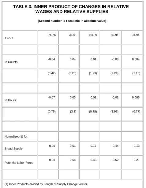
(10) WAGE DISPERSION AND TRADE IN ARGENTINA. We also calculate a normalized inner-product. We normalize the inner-product by the length of the vector of supply changes. This allows us to compare the measures across intervals and, potentially, across countries. To minimize sampling error inner products are calculated using both annual and three-year centered averages of quantity and wage vectors (Similar results were found, and those based on the centered averages data are reported). TABLE 3. INNER PRODUCT OF CHANGES IN RELATIVE WAGES AND RELATIVE SUPPLIES (Second number is t-statistic in absolute value). YEAR. In Counts. In Hours. 74-76. 76-83. 83-89. 89-91. 91-94. -0.04. 0.04. 0.01. -0.08. 0.004. (0.42). (3.20). (1.93). (2.24). (1.16). -0.07. 0.03. 0.01. -0.02. 0.005. (0.75). (3.3). (0.75). (1.93). (0.77). 0.00. 0.51. 0.17. -0.44. 0.13. 0.00. 0.64. 0.43. -0.52. 0.21. Normalized(1) for:. Broad Supply. Potential Labor Force. (1) Inner Products divided by Length of Supply Change Vector. In Table 3 above we see that the Inner Products for counts and hours went from negative but not significant values in 1974-1976 to positive and significative values in 1976-1983, and positive but not significant values in 1983-1989 and between 1991-1994. These results suggest that relative supply movements were not sufficient to explain relative wage changes before 1989 and after 1991. RELATIVE DEMAND In the last subsection, we presented evidence suggesting that, during both trade liberalization attempts, in Argentina relative demand shifted towards more skilled workers. In this sub-section, we directly estimate relative demand shifts. To do this we examine the time-series of relative wages and the constructed time-series of relative supply, then net-out relative supply shifts from relative wage changes to get estimates of the time-series of relative demand shifts. We find rising relative demand after 1976, from 1986 to 1989 and after 1993, suggesting that relative demand became skill-biased in those periods. In this time-series framework we also test whether changes in minimum wages or the skill composition of unemployed workers were responsible for relative wage shifts. The approach employed builds upon Freeman (1975, 1979, 1980) and follows KM92. For a simple CES production function we may write relative wage shifts as a function of relative demand and supply shifts, and the elasticity of substitution between more (1) and less (2) skilled workers: Page 10.
(11) WAGE DISPERSION AND TRADE IN ARGENTINA. (5) log(W1,t/W2,t) = (1/σ ) [dt - log(s1,t/s2,t) ], or w t = (1/σ ) [dt - st] where W i,t and si,t are, respectively, wages and supplies of group i in time t; and where wt, st and dt are relative wages, supplies and demand shifts at t, and σ is the elasticity of substitution between type one and type two workers. Freeman originally estimated this equation using simple supply measures and manpower (fixed input-output coefficients) extrapolations of demand shifts. We incorporate a more complete supply measure and employ a different estimation strategy reflecting that both the elasticity of substitution and demand shifts are unobserved. We proceed in three stages. First we construct the time-series of relative wages and supply (see previous section). Second, we estimate equation (5), above, approximating demand by a linear trend to obtain bounds on the elasticity of substitution, and test the impact upon relative wages of some other time-varying variables. Third, we calculate the time-series of relative demand assuming differing elasticities of substitution. Estimates of equation (5) assuming a linear trend for demand yield implied elasticities of substitution between 1.1 to 2.0. Broader supply measures including unemployed workers, or even the entire potential labor force had little effect on the estimates of the elasticities of substitution. To impute demand we solve (5) for dt and calculate dt assuming a range of elasticities of substitution around the estimated values from Stage Two. Thus, (6) dt = σ ×w t + st, and the imputed demand series using elasticities equal to 1.1 and 1.5 (the same qualitative results hold for a wide range of elasticities) are presented in the figure below. The point we wish to emphasize is that estimated relative demand did not fall neither with the first attempt of trade liberalization nor during most part of the second one. We see that estimated relative demand rose after 1976 until 1980, from 1986 to 1989 and after 1993, contrary to HOS-X. That is, trade liberalization in the mid seventies and in the mid eighties did not lead to a decrease in demand from more-skilled workers as predicted by HOS-X. The rise of relative demand between 1986 and 1989, along with the increase in relative wages and relative supply is an important point. During this period, workers with higher education were more fully indexed, so that accelerating inflation would have wide wage differentials, even when the relative demand had have not changed. But, the fact that relative. demand was skilled biased goes against HOS-X predictions. However, after 1989, when the trade liberalization was profounded by the new democratic administration, relative demand decreased from 1989 to 1990, then increased from 1990 to 1991, decreased slightly until 1993 to rise in 1994. In the same period, relative wages followed the same pattern, but relative supply remained stable between 1989 and 1990, then rose from 1990 to 1991 and then decreased in 1992 and rose after 1993. It's worth mentioning that is very difficult to isolate true trade effects from high inflation effects Page 11.
(12) WAGE DISPERSION AND TRADE IN ARGENTINA. over relative wages during the 1989-1991 period. However, it not seems clear that predictions of HOS-X are supported by the data; trade liberalization in Argentina was not consistent with HOS-X predictions. ALTERNATIVE EXPLANATIONS Before turning to an analysis of the causes of the skill-biased relative demand shifts, we briefly discuss four non-demand-based interpretations of the shifts in relative wages. These explanations are: minimum wages; mis-measurement of relative supply; unions; and changing schooling quality. Minimum Wages - To control for the impact of minimum wages on relative demand, we include in the estimation of equation (5) a minimum wage time series designed to capture its impact on relative wages. We tried several specifications of equation (5) including as independent variables measures of exports, imports and GDP. The estimated coefficient on the minimum wage variable was consistently insignificant, and lead us to reject minimum wage policy as the cause of relative wage shifts. Skill composition of the Unemployed (Mis-measurement of relative supply)- If the relative supply of skill were mis-measured, a biased estimate of relative demand shifts would result. This might occur because the definition of relative supply was too narrow. We tested this by using various measures of relative supply: first, including employed, self-employed, unpaid family workers and unemployed workers; second, adding discouraged workers; and third, adding all persons above fifteen years of age. We also controlled for the unemployment rate. The results were robust to these different supply measures, and the inclusion of the unemployment rate. Unions - It is unlikely that changes in union strength could explain the rising relative wages and estimated relative demand after 1976. As we mentioned in Section I, the political project of the military regime was to discipline the labor force. In order to do this, the military administration adopted several measures, such as to freeze wages, to forbid protests and to place under government control workers' unions. Therefore, workers' unions influence declined or even disappear after the military seized power. Between 1986 and 1989, union strength rose, but most unionized workers in Argentina are primarily low skilled workers, therefore if changing union power were the cause of changing relative wages, we should have observed a decline and not an increase in them. We controlled for the effect of unions on relative demand by including, in the estimation of expression (5), a dummy variable reflecting the strength of unions. The estimated coefficient on this dummy variable was statistically insignificant. Educational Quality - If the relative quality of university education rose after 1976, this could explain rising relative wages and the estimated relative demand. If this were the case we would not expect to see rising relative wages after 1976 for workers in the same age cohort. Table 5 reports relative wages over time for the cohort of males and females entering the labor force in TABLE 4. Ratio of University to Primary Wages for the Cohort of 1975 Labor Force Entrants.. 1975. 1980. 1985. 1990. 1994. MALES. 1.92. 3.06. 3.26. 3.08. 3.17. FEMALES. 2.37. 3.38. 2.56. 3.92. 2.30. Note: Calculated from desegregated normalized wage matrix, aggregating across experience and sub-groups of schooling using constant demographic weights.. 1975. Because for both men and women, relative wages rose rapidly after 1975, we conclude it is unlikely that schooling quality changes can explain rising relative wages and estimated relative demand during the first liberalization episode. The pattern of changes is less clear since 1985, however is highly improbable that an increase or decrease in the quality of education could affect males and females in a different way. Overall, it seems that non-demand-based factors that might have biased our relative demand estimates do not appear able to explain the rising estimated relative demand shifts. Therefore, the most plausible explanation is that demand did become skill-biased after 1976 and after 1986, coincident with trade liberalization. Next, we examine Page 12.
(13) WAGE DISPERSION AND TRADE IN ARGENTINA. the nature and causes of these relative demand shifts. IV. NATURE AND CAUSES OF RELATIVE DEMAND SHIFTS In this section we probe further into the nature and causes of relative demand shifts. First, we construct a decomposition of employment shifts into between- and within-industry shifts. We use the decomposition of employment shifts to examine whether relative demand changes are consistent with HOS-X. Then we examine the causes of the changes in relative demand. We do the latter by regressing the time-series of implied relative demand shifts, derived in Section III above, onto trade flows and other controls. Decomposition of Demand Shifts According to HOS-X, trade should lead to output and employment shifts "between" sectors from skill-intensive to unskilled intensive sectors, or unskilled-intensive between-industry shifts. HOS-X also predicts that these between-industry shifts will induce lower relative wages. In response to lower wages, within industries and firms, there will be a second order increase in skill intensity, or "within-industry" skill-intensive shifts. In this section we desagregate employment shifts into between and within-industry changes. To decompose employment shifts into overall, between-industry and within-industry shifts, we employed the methodology advanced in KM92. That methodology is a generalization of the standard fixed-coefficients index. The difference from Freeman's approach is that first, employment is measured in constant-valued efficiency units instead aggregating across experience and sub-divisions of schooling levels using counts of workers or hours worked (see KM92, Freeman 1975, 1979, 1980). Second, data on employment distributions within activities by occupations are used to estimate within-industry employment and demand shifts. "Overall" employment shifts are measured using average manning ratios within industries and occupations, and calculating the projected employment changes from shifts in both industry and occupational employments. Between-industry changes are measured by projecting changes in the composition of employment from shifts in the employment pattern across industries. "Within" changes are then calculated as the difference between "overall" and "between" changes. More formally, the between-sector change in demand for group k measured relative to base year employment of group k in efficiency units, EK is: (7) ∆ X kd = ∆ D K/EK = Σ j (Ejk/Ek) (∆ E j /Ej ) = Σ j α jk∆ E j /Ek, for the jth sector. Here Ej is the labor input in the jth sector in efficiency units,α jk (=Ejk/Ej ) is group k's share of total employment in efficiency units in the jth sector in the base year, which we normalize into an index of relative demand shifts using employment measures so total employment in efficiency units sums to one in each year. This formulae is used to calculate the three groups of demand shifts: the overall demand shifts, by letting "j" vary over both industries and occupations; between-industry demand shifts, by letting "j" vary only over industries; and within-industry shifts as the difference between overall and between shifts. Table 5 reports the findings, separately for men and women. Panel one reports overall shifts, panel two reports between-industry shifts and, panel three reports within-industry shifts The increase in demand from 1976 to 1985 was caused by an increase in the relative demand for more skilled men and women (overall shifts were positive for both). This increase in demand was driven by between industry shifts towards more-skilled male and female workers. Within industry changes were towards more-skilled male workers only in the period 1978-1983. On the contrary, the increase in demand from 1985 to 1989 was driven by within industry shifts. These results are not consistent with HOS-X. The same observation can be made after 1991, when besides the skilled-intensive between industry shifts for males, these shifts were dominated TABLE 4. DECOMPOSITION OF EMPLOYMENT CHANGES (Data pertains to employed workers, self-employed, proprietors and unpaid family workers). Overall changes. SEX. SCHOOL. 74-76. 76-78. 78-83. 83-85. Page 13. 85-89. 89-91. 91-94.
(14) WAGE DISPERSION AND TRADE IN ARGENTINA. Males. Females. Primary. 0.00. -0.06. -0.27. -0.04. -0.11. -0.09. -0.09. Secondary. -0.04. -0.03. 0.05. 0.00. 0.00. -0.15. -0.17. University. -0.27. 0.05. 0.72. 0.08. 0.20. 0.16. -0.70. Primary. 0.08. -0.02. -0.43. -0.03. -0.29. -0.01. 0.44. Secondary. 0.32. 0.11. -0.41. 0.03. -0.15. 0.07. 1.34. University. 0.07. 0.13. 0.33. 0.16. 0.16. 0.22. -0.12. Between changes. SEX. Males. Females. SCHOOL. 74-76. 76-78. 78-83. 83-85. 85-89. 89-91. 91-94. Primary. -0.18. -0.14. -0.62. -0.24. 0.18. -0.20. -0.03. Secondary. 0.01. -0.06. -0.10. -0.03. 0.07. -0.41. 0.29. University. 0.16. 0.24. 0.47. 0.46. -0.53. 0.17. 0.03. Primary. -0.30. -0.28. 0.02. -0.17. -0.60. 0.13. -0.37. Secondary. 0.21. 0.19. 0.62. 0.30. -0.27. 0.45. -0.12. University. 0.38. 0.62. 1.21. 0.69. -0.13. 0.94. -0.45. 83-85. 85-89. 89-91. 91-94. Within Changes. SEX. SCHOOL. 74-76. 76-78. 78-83. Page 14.
(15) WAGE DISPERSION AND TRADE IN ARGENTINA. Males. Females. Primary. 0.18. 0.08. 0.35. 0.21. -0.30. 0.12. -0.06. Secondary. -0.05. 0.03. 0.16. 0.03. -0.07. 0.26. -0.46. University. -0.43. -0.19. 0.25. -0.38. 0.72. -0.01. -0.73. Primary. 0.39. 0.27. -0.45. 0.13. 0.31. -0.15. 0.82. Secondary. 0.11. -0.08. -1.03. -0.26. 0.12. -0.38. 1.46. University. -0.31. -0.50. -0.87. -0.53. 0.30. -0.72. 0.33. in magnitude by the within industry changes. For females, during this period, between industry changes were negative, while within industry shifts were positive for all educational groups. Between 1985 and 1989, the increase in relative demand was caused by within changes. For males, there was an skill-intensive within industry shift but this was not the case for female workers. Overall, the decomposition of employment shifts provides additional evidence that HOS-X cannot explain employment shifts caused by trade liberalization in Argentina. Correlates of Relative Demand Shifts In Section III we found that the estimated time-series of relative demand shifts rose during the first attempt of trade liberalization and during most years of the second one, in Argentina. In this section we examine the correlates of these demand shifts to shed more light upon their causes, in particular in relation to trade variables. We model relative demand shifts here as potentially affected by GDP, trade flows as percents of GDP, and a measure of the stock of machinery imported relative to GDP. Ex ante, there is no particular reason or evidence why relative demand should follow a trend. For example, while most U.S. economists now believe that the rising relative demand after 1980 was due to skill-biased technological change, Katz and Goldin (1995) have shown that technical change is not always skill biased. Ex-ante we would expect balanced economic growth to lead to skill-neutral labor demand. HOS-X is a theory of unbalanced growth, where unskilled-labor-intensive LDCs should produce and export unskilled-labor-intensive products. Therefore, trade liberalization in LDCs like Argentina should lead to unbalanced growth biased towards these unskilled-labor-intensive sectors. Trade liberalization in LDCs is expected to induce unbalanced growth in the form of higher imports and higher exports to GDP. On the other hand, the Skill-Enhancing Theory (e.g. Stokey, 1994; Park and Page, 1993) suggests a channel by which trade liberalization could induce rising relative demand - by raising the imported capital/GDP ratio, tending to raise the overall capital/GDP ratio and serving to accelerate the transfer of skill-biased technology from developing countries. To control for the SET effect we included estimates of the stock of imported machinery divided by GDP. More explicitly, we employ the time-series of imputed relative demand, discussed above in Section III. Recall that relative demand was estimated above as: (8) dt = σ ×w t + st, where rough bounds on s were obtained by regressing relative wages onto a trend and the constructed relative supply. We then estimate equations of the form: (9) dt = f(x, m, ICS, GDP). Page 15.
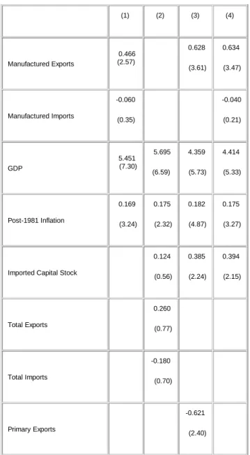
(16) WAGE DISPERSION AND TRADE IN ARGENTINA. where "x" are measures of export flows divided by GDP, "m" are measures of import flows divided by GDP, and "ICS" is the imported capital stock divided by GDP. Trade flows for exports and imports were taken from the World Bank's World Tables, while imported capital stock was constructed from the COMTRADE data base. The results were not sensitive to different depreciation rates (here we report using a 20% rate). Various specifications were estimated. Table 6 below reports representative findings for regressions of imputed relative demand onto logged trade flows, log(GDP) and log(ICS). F-statistics are high, ranging from 11.24 to 29.86, and adjusted R-Squares from 0.73 to 0.90. The principal finding is that log(GDP) and log(ICS) have large positive coefficients that are statistically significant at conventional levels. The estimated coefficients on log(ICS) ranged from .34 to .39, with t-statistics ranging from 2.15 to 2.39. We include log(GDP) principally as a control in studying the effects of trade-related variables upon relative demand. Here we find that estimated coefficients on log(GDP) are consistently positive. They range from 1.66 to 5.69, while t-statistics range from 1.43 to 7.30. TABLE 6. CORRELATES OF IMPLIED RELATIVE DEMAND (Estimated using Ordinary Least Squares) Dependent Variable: Imputed Relative Demand For Skill (1). Manufactured Exports. Manufactured Imports. GDP. Post-1981 Inflation. (2). 0.466 (2.57). (3). (4). 0.628. 0.634. (3.61). (3.47). -0.060. -0.040. (0.35). (0.21). 5.695. 4.359. 4.414. (6.59). (5.73). (5.33). 0.169. 0.175. 0.182. 0.175. (3.24). (2.32). (4.87). (3.27). 0.124. 0.385. 0.394. (0.56). (2.24). (2.15). 5.451 (7.30). Imported Capital Stock. 0.260 Total Exports. (0.77). -0.180 Total Imports. (0.70). -0.621 Primary Exports. (2.40). Page 16.
(17) WAGE DISPERSION AND TRADE IN ARGENTINA. Adj. R-Squared. F-Statistic. Durbin-Watson. N. 0.80. 0.73. 0.85. 0.84. 20.70. 11.24. 23.20. 18.03. 2.00. 1.78. 2.21. 2.23. 21. 21. 21. 21. Notes: Absolute value t-statistics in parentheses. Independent variables in logs, trade variables divided by GDP.. The coefficient on post 1981 inflation is positive and statistically significative implying that during the 80s inflation had a positive impact upon relative demand. The results for the trade flow variables are statistically weaker, but suggestive of a heterodox SET result. They are weakly consistent with HOS-X for imports and strongly inconsistent for exports. The coefficients on the log of import flows to GDP are negative but not significative, so these findings are weakly consistent with HOS-X. Primary-non-fuel exports, associated with agricultural production, would typically be intensive in unskilled labor, so that their negative coefficients do fit HOS-X predictions. These patterns are similar to those found for Colombia and Chile (Robbins 1995a 1995b). We interpret these findings cautiously as consistent with the SET hypothesis, while offering mixed results regarding direct factor content of trade effects along HOS-X. The SET hypothesis is supported by the positive, significant and stable estimated coefficients on Imported Capital Stock. The tendency for export to GDP ratios to be positive goes against HOS-X. GDP growth appears to raise relative demand, but it does not affect most other coefficients, in particular those on the ICS variable. V. CONCLUSIONS Our analysis of the Argentine trade liberalization experience does not support HOS-X. HOS-X would predict lower relative demand and hence relative wages, by inducing between-sector shifts towards sectors intensive in unskilled labor. For Argentina, relative supply rose continually throughout the period studied, while subsequent to trade liberalization relative wages stopped falling and began to rise, suggesting skill-biased relative demand shifts. Estimated time series of relative demand showed a marked rise after trade liberalization. This appears to have been driven largely by product and employment shifts towards skilled sectors, contrary to HOS-X. Analysis of the correlates of relative demand shifts suggests a somewhat heterodox interpretation. Total imports and imports of manufactures are associated with lower relative demand, along the lines of HOS-X, although they are not statistically significant. Against HOS-X, we find that total exports and particularly exports of manufactured products are positively associated with relative demand. Growth and imported capital stock, though, appear much more important in determining relative labor demand. Economic growth and rising stock of imported machinery may be important causes of the skill-biased relative demand shifts after trade liberalization. Thus, we find very little support for HOS-X, and some support for the SET hypothesis, whereby trade liberalization induces an acceleration of physical capital imports, which through capital-skill complementarily raise relative demand. References. Canitrot, Adolfo, "Teoría y Práctica del Liberalismo. Política Antiinflacionaria y Apertura Económica en la Argentina, 1976-1981", Desarrollo Económico vol. 21, no. 82, julio-septiembre, 1981: 131-189. Damill, Mario and Saul Keifman, "Liberalización del Comercio en una Economía de Alta Inflación: Argentina 1989-1991", Pensamiento Iberoamericano no. 21, 1992: 103-127 Freeman, Richard B., "Overinvestment in College Training," Journal of Human Resources vol. 10, no. 3, 1975: 287-311. Freeman, Richard B., "The Effect of Demographic Factors on Age-Earnings Profiles", Journal of Human Resource, vol. XIV, no. 3, 1979: 290-318.. Page 17.
(18) WAGE DISPERSION AND TRADE IN ARGENTINA. Freeman, Richard B. , "An Empirical Analysis of the Fixed Coefficient Manpower Requirements Model, 1960-1970," Journal of Human Resources, Vol. XV, no. 2, 1980. Freeman, Richard. B, "Demand for Education", in: Handbook of Labor Economics, Ashenfelter, et al, eds., Vol.I, 1986: 359-386. Grossman, Gene M. and E. Helpman, "Innovation and Growth in the Global Economy", The MIT Press, 1991. Katz, L. and C. Goldin, "The Decline of Non-Competing Groups: Changes in the Premium to Education 1890-1940", mimeo, Harvard University, 1995. Katz, L. and K. Murphy, "Changes in Relative Wages, 1963-1987: Supply and Demand Factors",Quarterly Journal of Economics, vol. CVII, February 1992: 35-78. Krueger, Anne O., "The Relationships Between Trade, Employment, and Development," with comment by Michael Bruno, in: Ranis and Schultz eds., The State of Development Economics: Progress and Perspectives, Cambridge, MA, Basil Blackwell, 1990: 357-385. Menendez, Alicia, "Relative Wages and Inflation. Argentina 1974-1993", mimeo, Boston University, 1996. Murphy, Kevin M. and Finis Welch, "The Role of International Trade in Wage Differentials," in: Kosters, ed.,Workers and Their Wages: Changing Patterns in the United States, Washington, D.C.: The American Enterprise Institute Press, 1991: 39-69. Pessino, C and L. Giacchino, "Rising Unemployment in Argentina: 1974-1993", mimeo. Robbins, Donald, "Human Capital, Growth, Trade and Wage Dispersion -Greater Bogotá, Colombia: 1976-1989-", mimeo, Harvard University, June, 1995. Robbins, Donald, "Trade Liberalization and Earnings Dispersion -Evidence from Chile-", mimeo, Harvard University, May, 1995. Stokey, Nancy, "Free Trade, Factor Returns and Factor Accumulation," mimeo, University of Chicago, March 1994 Welch, Finis, "Effects of Cohort Size on Earnings: The Baby Boom Babies' Financial Bust,"Journal of Political Economy, LXXXVII, October 1979, S65-98.. Page 18.
(19)
Figure


+3

Documento similar