Economic and socio demographic determinants of crime in Uruguay

Texto completo

(1)Este documento forma parte de la producción editorial de la Conferencia Interamericana de Seguridad Social (CISS) Se permite su reproducción total o parcial, en copia digital o impresa; siempre y cuando se cite la fuente y se reconozca la autoría..

(2)

(3) WELL-BEING AND SOCIAL POLICY VOL 6, NUM, 2, pp. 45-73. ECONOMIC AND SOCIO-DEMOGRAPHIC DETERMINANTS OF CRIME IN URUGUAY* Fernando BorrazBCU-Departamento de Economía, FCS, UDELAR fborraz@bcu.gub.uy. Nicolás González*" Universidad de Montevideo ngonzalez@correo.um.edu.uy. Abstract. T. his study estimates a panel data model to analyze the economic and socio-demographic determinants of crime in Uruguay across the 19 Uruguayan departments in the period 1986-2006. This research has two components: i) to present a systematic analysis of the Uruguayan crime data and socio-economic and demographic characteristics of the population, and ii) to evaluate the empirical significance in Uruguay of the economic crime model developed by Becker (1968) and Ehrlich (1973) with the objective to explain why the crime rate varíes over time and across departments. We estimate a dynamic panel data model to identify the socio-economic and demographic determinants of crime. In the estimation we include department fixed effects which captures non observable heterogeneity. Also, we study the hypothesis of crime inertia by including the lagged crime rate as exploratory variable. The generalized method of moment methodology allows us to control for endogeneity in some explicative variables and for the existence of correlated measurement error in crime statistics. Our results are as follow: i) the socio-economic factors have no significant effect on the crime rate; ii) an increase in the crime rate tends to perpetuate overtime; iii) the population density and urbanization rate positively affects crime; and iv) the deterrent factors are relevant to reduce crime against property. Keywords: crime, dynamic panel data model, deterrence, Uruguay. JEL classification: D33, J60, C23.. • The opinions expressed here are those of the authors and do not necessarily reflect the positions of the Banco Central del Uruguay and the Universidad de la República. We thank participants at the conference "Crime and Violence in Latin America and the Caribbean" organized by the Inter-American Conference on Social Security, the CAF and UNDP Mexico, in Mexico, October 1", 2010. We also wish to thank Rodrigo Soares and Daniel Ortega for useful comments. Any error is our responsibility. ** Banco Central del Uruguay. Diagonal Fabini 777, CP 11,100. Montevideo, Uruguay. *** Universidad de Montevideo. Prudencio de Pena 2440, CP 11,600. Montevideo, Uruguay.. 45.

(4) ECDNOMIC AND SOCIO-DEMOGRAPHIC DETERMINANTS OF CRIME IN URUGUAY. Introduction. A. ccording to the World Bank (1997): "Crime and violence are obstacles to economic growth and poverty reduction because their effect in physical, human and social capital, and their harmful impact in government capacity building. The combine result of these negative effects of crime and violence is a reduction in economic growth and an increase in poverty". Until the seventies crime was explained by individual deviated behaviors and atypical motivations. The crime theory was formed by a set of recommendation of sociologists, psychologists, and lawyers based on the concept of abnormality. The crime started to be analyzed from an economic perspective since the innovator work of Becker of 1968. The Becker's dissuasion theory is an application of the general theory of rational behavior under uncertainty. According to Becker (1968): "Some persons become "criminals", therefore, not because their basic motivation differs from that of other persons, but because their benefits and costs differ". Becker assumes that agents are function maximizers. For example, consumers maximize their utility function. Therefore, he predicts that people will commit a crime when the expected utility of crime is higher than the expected utility to dedicate to legal activities. In this way, he established a rational behavior model of crime which is the base of the crime economic approach. Criminals behave rationally and they realize a cost benefit analysis of their activities. Ehrlich (1973) developed a time allocation model. He started assuming individuals with a fixed leisure time. Hence, they had to decide to allocate the rest of their time into legal or illegal activities. When income opportunities in legal activities are low, the time allocation model predicts an increase in crime. Additionally, Ehrlich (1973) realized empirical research based on Becker's theoretical model. Because income opportunities in legal activities can be approximated by family income and other socio-economic variables (unemployment, age, etc.) the Ehrlich's prediction model can be tested empirically. Consequently, there is a set of socio-economic and demographic variables that affect the expected cost and benefit of crime and they can be considered as determinants of crime. For example, income opportunities in legal activities should impact the decision to commit or not a crime. In base of Becker (1968) and Ehrlich (1973) approach this paper estimates a panel data model to analyze the economic and socio-demographic determinants of crime in Uruguay. We collect an important set of crime information in Uruguay by department. In particular, we obtain the reponed quantity of crime in Uruguay by crime type: against the person or the property. Moreover, we process the Uruguayan household surveys to have information about economic and sociodemographic variables by department.. 46.

(5) WELL-BEING AND SOCIAL POLICY VOL 6, NUM. 2, pp. 45-73. The empirical test of the economic model of crime implies an econometric estimation to explain the economic and socio-demographic determinants of crime in Uruguay by department between 1986 and 2006. We estimate a dynamic panel data model by the generalized method of moments (GMM) and by the Kiviet (1995) method that allows us to control by department fixed effects, by endogeneity of some exploratory variables and by possible measurement error in crime statistics. We can also analyze crime inedia by including the lagged crime rate as explanatory variable. The results are as follow: i) the crime rate is not countercyclical; ii) the dissuasive effects are important; iii) the population density is highly correlated with crime rate; and iv) there is a positive inedia of crime. This paper is organized as follow. The first section presents an overview of crime trends in Uruguay. A brief review to the economic of crime literature and a simple model of crime incentives is developed in section two. In the third part of the paper we discuss the methodology used to estimate the determinants of crime. The fourth section shows the estimation results. Finally, we present the conclusions.. 1. Overview of Crime Trends in Uruguay Figure 1 shows the evolution of total crime per 1,000 inhabitants in Uruguay in the 1986-2006 period. In a two decades period the crime rate per 1,000 inhabitants doubled, increasing from 21.7% in 1986 to 40.3% in 2006. In this period we can distinguish two sub-periods: i) from 1986 to 1998, where we observe an oscillation in the crime rate around the level of 20 per 1,000; and ii) between 1999 and 2006, where there is a substantial increase in the crime rate. For this last sub-period the average growth rate of crime is 15% per year. This positive long term trend in the growth rate of crime is consistent with Fajnzylber, Lederman, and Loayza (1998) who fmd a sustained increase in the homicides and thefts since the seventies for a set of 120 countries. They conclude that this positive trend is explained by crime in low and medium-low income countries.. 47.

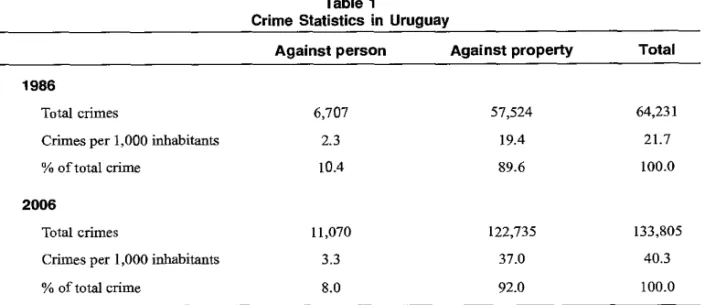
(6) ECONOMIC AND SOCIO-DEMOGRAPHIC DETERMINANTS OF CRIME IN URUGUAY. Figure 1 Crime Rate per 1,000 Inhabitants. 45 40 35 30 25 20 15 00 N en 01- 01 10 N ro 01- 01 0 r- 00 01 0 DO DO 00 00 a, 01 01 0 Ch 01 01 0, p, 0 0 0 000 00 0 0 0, 0, O, 01 01 Cr. 01 01 0 0, O, O 0 0 0 00 NI NI NI N N 00. Source: National Institute of Statistics (INE).. Table 1 indicates that crime against property is the type of crime with the highest proportion in total crime. Therefore, the steep raise in the crime rate can be explained by the sharp increase in crime against property.. Table 1 Crime Statistics in Uruguay Against person. Against property. Total. 6,707. 57,524. 64,231. Crimes per 1,000 inhabitants. 2.3. 19.4. 21.7. % of total crime. 10.4. 89.6. 100.0. 11,070. 122,735. 133,805. Crimes per 1,000 inhabitants. 3.3. 37.0. 40.3. % of total crime. 8.0. 92.0. 100.0. 1986. Total crimes. 2006. Total crimes. Source: National Institute of Statistics (INE).. 48.

(7) WELL-BEING AND SOCIAL POLICY VOL 6, NUM. 2, pp. 45-73. An important element to be considered is the fact that crime statistics reflect only the reported number of crime and not the effective total number of crime. This is the problem of underreporting and the official crime data underestimate the total number of crimes. This measurement error does not bias the estimation if the errors are not correlated with the explanatory variables and if they do not vary systematically per department. However, in this case we have arguments to think that the underreporting is correlated with exploratory variables. We analyze this issue deeper in the methodology section. For a better description and comprehension of the crime phenomena in Uruguay the Figures 2 and 3 show the disaggregation of total crime in crime against the physical person (aggressions and injuries, sexual crimes and homicides) and crime against property (thefts, rapines, and damages). We observe an important growth in crime against the person from 1986 to 1991. In 1992 we see a pronounced dip. After that, it remains stable from 1993 to 1998. Finally, we notice a return to growth since 1999.. Figure 2 Crime against Person per 1,000 Inhabitants 4.0 3.5 3.0. 2.5 2.0 L5. 00 OS nr ,e1 1/40 r- 00 OSO.-. 00 CO 00 00 05 CN ON T OS CN 0, 0100000000 0, 0, OS O, 01 0 O, ON P en 0,O, 05 O, 0 O 0 O 0 0 0. N N N N el N 1, 1. Source:. National Instituto of Statistics (INE).. 49.

(8) ECONOMIC AND SOCIO-DEMOGRAPHIC DETERMINANTS OF CRIME IN URUGUAY. Figure 3 Property Crime per 1,000 inhabitants. 40 35 30 25 20 15 c., cc, nj- 1sc, 'S> r- 00 Oh Cgrh,1r00 00 CO 00 01 Oh 01 Ch Ch a, 0/ 01 00000 0 01 01 01 01 01 T Ch Ch Ch 01 01 01 01 Ch 0 0 0 0 0 0 0 CV CV CV C4 fq CV N. Source: National Institute of Statistics (INE).. The crime against property presents a similar trend than the crime against person (see Figure 3). We observe a period of growth between 1986 and 1991, stability between 1992 and 1998, and growth again from 1999 to the present. It is remarkable that crime against property represents approximately 90% of total crime. However, such percentage must be higher because some crime against the persons, like homicides, could have origin in a crime against property. Additionally, the crime against property is the crime more directly related to the analysis of the economic model of crime. Therefore, in the estimation, we also report separate results for crime against property and crime against person. Figures 1-3 do not consider crime variation across departments. Figure 4 shows the crime rate per 1,000 inhabitants by departments for the years 1986 and 2006. A first look indicates that in almost all Uruguayan departments we observe an increase in the crime rate in the period under analysis. The average growth rate for the period is 4.1% per year. The highest growth rates are observed in Migas (12.1%), Treinta y Tres (9.4%), and Río Negro (8.6%). The average growth rate in the capital Montevideo City is 4.1% per year. On the other side, the lowest crime growth rate are in Cerro Largo (-2.1%), Durazno (-0.9%), and Florida (0.4%). A second conclusion from Figure 4 is the high dispersion observed in crime rate against property across departments. For the year 2006, such crime rate varíes from 6.9% in Cerro Largo to 60.0% in Maldonado. Figure 5 presents the log crime rate within variation across departments by year. Each dot represents a department's crime rate less their mean, in other words, the deviation from their means.1 The curve line is fltted by OLS of the (log) crime rate on year dummies From the figure we Suppose that the variable y represent the log crime rate. Then, the deviation from the mean is calculated as Ti follows: (yit — yi + y) with i= 1,...,19 t= 1986,...,2006, where i is the department, and t is the year; yi = Ti E Yit and y is the overall mean. We add the overall mean in order to preserve the scale.. 50.

(9) WELL-BEING AND SOCIAL POLICY VOL 6, NUM. 2, pp. 45-73 Figure 4 Crime Rate by 1,000 Inhabitants per Department 60 50 40 30 20 10. 1 1 NEME 111~I MINI I M'II. o <juulz 1.11P: FC 1 • 1986. • 2006. Source: National Institute of Statistics (INE).. Figure 5 Department within Variation of Log Crime Rate by 1,000 Inhabitants. •. en. 1,1. al e .e .:11111 , ,...,, e .• • • , •e 1 ••••1¡,...-1", • e , e 1..3 1- ..!. • 1...-0 1 • : . • • le ele J...1-1-1 í e:4 14/1~ 1 : • t.:. • il t 11 i . I .E . 1 .1 e , • I i ••.e ,.. .• ..* 1986. 1990. 1994. 1998. 2002. 2006. Year • Log Crime Rate. — — — - Fitted values. Source: National Institute of Statistics (INE) and authors' calculation.. observe that there is a substantial variation as well as a positive trend that arise from the fitted values. Additionally, Figure 6 approximates better the dispersion across departments showing the coefficient of variation of total crime per 1,000 inhabitants. As we observe, there is an important dispersion of crime across departments. Therefore, there is much to explain with panel data estimation. The evidence shows that the coefficient of variation is higher than 0.35 in all of the years. This fact suggests that the incorporation of the time dimension can aggregate useful information in the estimations. 51.

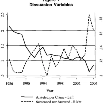
(10) ECONOMIC AND SOCIO-DEMOGRAPHIC DETERMINANTS OF CRIME IN URUGUAY Figure 6 Coefficient of Variation of the Property Crime Rate by Department. Coefficient of variation. .55. .5. 45. .4. .35 1986. 1990. 1994. I998. 2006. 2002. Year Source: National Institute of Statistics (INE) and authors' calculation.. Another element to be considered in the crime analysis is dissuasion (deterrence factors). Figure 7 shows the number of arrested divided by the number of reponed crimen and the probability of being sentenced defined as the number of sentenced divided by the number of arrested. The probability of being sentenced follows an oscillate path until 2003. After that, it increases from just over 0.12 in 2003 to 0.16 in 2006. On the other hand, the ratio of arrested to crime shows a downward trend throughout the whole period. Figure 7 Dissuasion Variables. CV. % I 1. I. e. e. l........1. 1986. 1990. i ` I. 1. 1 I S I 1I. a». 1998. 1994. 2002. 2006. Year Arrested per Crime - Left — — — — - Sentenced per Arrested-Right Source: National Institute of Statistics (INE) and Ministry of Interior (Ministerio del Interior).. 52.

(11) WELL-BEING AND SOCIAL POLICY VOL 6, NUM. 2, pp. 45-73. 2. The Economic Model of Crime 2.1 Theoretical developments The economic literature has started to build a specific theoretical framework to study crime since the pioneer work of Becker (1968). Based on the election analysis used by economist Becker states that a risk neutral agent will commit a crime if her expected utility of this activity exceeds the expected utility in legal activities. Therefore, some persons commit crime not because their basic motivations differ but because their benefits and costs are dissimilar. By this way, the economy considers crime as an alternative activity to the legal one and individuals choose rationally one or the other. In a broad sense we can define a rational behavior approach to study crime. According to the rational behavior model guided by norms, the decision to commit or not a crime depends on person desires and contexts, abilities and believes with respect to attainable outcomes (Eide 1994). The differences across two individual in these factors can explain why one person commits crime and the other not. When a person decides to commit a crime he or she causes damage to the society. To this, the society reacts with self protection. The moral and economic damage of crime on agents, the police apprehension costs, the justice costs, the jail expenditures, the opportunity cost of sentenced criminals, and the prevention private costs representa the social loss because of crime. One social objective is to minimize such loss and the control variables are: the amount spends in crime combat, the penalties, and how the trails and the penalties are implemented (Becker, 1968). These factors indirectly determine the probability that a crime is convicted, the quantity of crime and the social loss because of crime. Becker (1968) stated that the optimal policy against crime is not necessarily the one that arrest the maximum number of offenses possible at any expenditure levet but the one that minimize the social loss associated with crime. Also, Becker (1968) define an offense function that relates the number of crime committed by one person with the probability of being arrested and sentenced and with other variables that measure the cost in legal and illegal activities such as disposable income. The theoretical framework of Becker (1968) has been empirically addressed since the work of Ehrlich (1973). Following Ehrlich the economic literature of crime has been focus in the estimation of an offense function where the determinants of crime are: the probability and severity of penalties, expected income in criminal activities, the economic return to legal activities and other socio-demographic variables such as the urbanization cate. The focus of the contributions moved from the test of deterrent factors to the analysis of the economic and socio-demographic factors of crime.. 53.

(12) ECONOMIC AND SOCIO-DEMOGRAPHIC DETERMINANTS OF CRIME IN URUGUAY. 2.2 A simple incentive model to commit crime In this subsection we present a simple model of criminal behavionz As we mentioned aboye we assume that potential criminal behave rationally and they analyze the cost and benefits of their actions to commit crime. Equation (1) sets that for a given agent the net expected profit (nep) to commit a crime equals the expected payoffs. That is, the probability of not being caught (1 - p) times the amount of the income to be perceived in illegal activities (i), minus the costs to commit crime (c), minus the opportunity cost of illegal activities that is the monetary wage (w) to be received in legal activities, minus the probability of being caught times the penalty to be received (pe). nem= (1-p)i -c -w -p * (pe). (1). Also, it is assumed that individuals would not commit crime merely when the net expected payoff is positive because their present moral values prevent them to commit crime when the net expected payoff is positive. Therefore, we assume that the person decide to commit crime (cri=1) when the net expected payoff exceeds a threshold m. On the contrary, when the expected profit does not reach that threshold the persons does not commit crime (cri=0). cri=1 if nep>=m (2) cri =O if nep<m. 2.3 Empirical implementation There are two different approaches in the economic literature to test the crime theory and to study the incentives the individual's faces at the time to commit a crime: the use of micro or macro data. The first ones allow us to extract a rich and relevant set of diverse information. For example, we could calculate the probability of crime relapse giving the economics and socio-demographics person characteristics. Although the experiments should be the principal empirical implementation of the crime economic theory, for obvious reasons these studies are scarce. The research of the determinante of crime using micro data requires a random sample of the population of criminal and non criminal persons.. 2. The model is based on Fajnzylber, Lederman, and Loayza (1998).. 54.

(13) WELL-BEING AND SOCIAL POLICY VOL 6, NUM. 2, pp. 45-73. Taking in consideration the lack of micro crime data we decided to work with macro variables that approximated the individual determinants of crime. We have to point out that even though we will work with macro data we will be able to test literature hypothesis and derive important policy recommendations. We will estimate an econometric model with the crime rate as the dependent variable and as exploratory variables a set of variables considered determinants of crime that approximated the individual characteristics and deterrence factors. In particular, the response variable will be the total crime rate defined as the crime per 1,000 inhabitants per department and per year. Additionally, and as a robustness check, we estimate the model by type of crime: against person or property. The crime against property is closely related to the economic model of crime. We expect the deterrence variable to impact only the property crime because this type of crime is more related to the economic model of crime than the crime against the person. Next, we present the explanatory variables. The deterrence variables are very important because their impact of expected utility to commit crime. In his original work, Becker (1968) uses the probability of being sentenced and the severity of the penalties as deterrence variables. The highest the level of there explanatory variables the lowest expected utility to commit crime. As a proxy of deterrence variables3 we use the percentage of arrested per crime and the percentage of sentenced per arrested. We also use the number of cops per 1,000 inhabitants. The department economic level of activity and its growth rate are also relevant variables to be considered in the study of the rational decision to commit crime. The income variable has an ambiguous effect on crime rate. On one way, the greater level of activity translates into more employment and income opportunities in the formal sector and discourages crime. On the other side, the higher the economic level the higher the amount of the benefit in illegal activities. Therefore, the relationship between economic activity and crime is ambiguous. The activity level is approximated by the real average household per capita income by department. Also, we have to consider the effect of unequal distribution of income on crime. We expect higher incentives to crime in departments with more unequal income distributions. Therefore, we estimate the Gini index at the department level. Other important variable to analyze opportunities in legal activities is the labor market situation. The crime empirical literature4 usually works with the unemployment rate as explanatory variable. This unemployment variable affects income opportunities of individuals making legal activities. It also contributes to depreciate quickly human capital of persons and decrease the possibility of income in the future, and therefore there is an increase in the net expected payoff of committing illegal activities.. We can not construct a variable that reflects the penalties severities given the fact that there is crime that is sanctioned without jail or only with fines. 3 Fajnzylber, Lederman, and Loayza (1998) and Raphael and Winter (1998). 3. 55.

(14) ECONOMIC AND SOCIO-DEMOGRAPHIC DETERMINANTS OF CRIME IN URUGUAY. We will work with the unemployment rate of people under 30 years old since youth are more prone to be involved in illegal activities (Grogger 1998). According to Egozcue (1999) a high percentage of the jail population is composed by men lower than 30 years olds. This evidence suggests that we have to use the percentage of mate population less than 30 years old at the department levet by year in the econometric estimation. Also, it is possible that young persons commit more crime because they are poorer than others. If we incorporate the income variable we will capture the pure effect of being youth. We also include as explanatory variables a set of socio-demographic variables such as: urbanization grade and population density.5 The crime empirical literature6 finds that crime is affected by the degree of urbanization in the cities. In particular, there is found a significant and positive correlation between city size and crime rate. Probably, the urban centers ease the social interaction and in this way they can facilitate the transmission of illegal activities and therefore there is a decrease in the cost to commit crime. Also, if the cities have higher population there is a lower probability of being captured, lower social punishment, etc. Therefore, we will use as explanatory variables the urbanization grade and the population density. As a synthesis Table 2 shows descriptive statistics of the dependent variable and independent economic and socio-demographics variables that will be used in the estimation of the dynamic panel data model.. 2.4 Lagged dependent variable — crime inertia hypothesis The past of individuals in crime activities is an important variable in the decision to commit a crime. Crime today can be associated with crime tomorrow in different ways. First, those who had committed illegal activities and had been captured and sentenced had less labor market insertion possibilities than those who had not committed crime. For example, Grogger (1998) finds that convicted criminals have less job opportunities in the legal labor market and a lower expected wage. Therefore, the formers face a lower opportunity cost to commit crime since their lack of access to legal activities and a legal source of income. Leung (1995) states that past criminal activity decline the probability of being employed in the legal labor market because of the "stigma" and depreciation of the human capital levet. Hence, once an individual commit a crime the probability of this same individual to be involved in criminal activities increase. In addition, we have to take into account that there is an important learning component of crime activities that notably reduces the cost of commit crime (Kling, Ludwig, and Katz 2004), in other words, there is a "learning-by-doing" component in criminal behavior. Once we know how to do it, it is much easier to do it again.. Inhabitants per squared kilometer. Glaeser and Sacerdote (1996) and Glaeser, Sacerdote, and Scheinkman (1996).. 56.

(15) WELL-BEING AND SOCIAL POLICY VOL 6, NUM. 2, pp. 45-73. Table 2 Descriptive Statistics Variable. Observations. Mean. Std. Dev.. Min. Max. Crime Rate. 399. 18.91. 9.97. 4.47. 60.89. Crime Rafe Against Person. 399. 2.93. 2.13. 0.18. 20.17 19.81. Crime Rate- Aggression and Injurie. 399. 2.65. 2.08. 0.08. Crime Rate- Sexual Crime. 399. 0.22. 0.15. 0.00. 1.72. Crime Rate- Homicide. 399. 0.06. 0.04. 0.00. 0.24. Crime Rate Against Property. 399. 15.98. 9.18. 3.53. 55.82. Crime Rate- Theft. 8.17. 3.23. 50.98. 399. 14.06. Crime Rate- Rapine. 399. 0.33. 0.78. 0.00. 5.85. Crime Rate- Damage. 399. 1.60. 1.12. 0.00. 8.99. Arrested per Crime. 399. 1.29. 0.93. 0.20. 8.46. Sentenced per Arrested. 399. 0.13. 0.08. 0.01. 0.68. Real per Capita Income (1997 Uruguayan pesos). 399. 2554.39. 639.74. 1414.70. 5353.39. Head of Household' s Education. 399. 6.91. 0.73. 5.37. 9.99. Gini Index. 399. 0.39. 0.04. 0.26. 0.64. Youth Unemployment (.29 years old). 399. 0.21. 0.08. 0.03. 0.51. Urbanization Rate. 399. 0.86. 0.05. 0.70. 0.97. Population Density. 399. 147.52. 566.37. 4.74. 2604.72. Border Dummy. 399. 0.21. 0.41. 0.00. 1.00. Source: National Institute of Statistics (INE).. Third, Sah (1991) studies the dynamic relationship of criminal behavior in order to uncover the determinants of the crime rate and find out if it follows a partem which could explain its evolution. He argues that there is a strong link between the level of the crime rate and the probability of punishment. In that sense, regions with high crime rates can be associated with a low probability of being caught and regions with low crime are associated with a low level of deterrent factors. A high crime rate could perpetuate overtime if the deterrent factors remain unchanged. Forth, we presentan argument that is strongly theoretical and empirically supported and it is based on the concept of "social interaction". Authors like Glaeser, et al. (1996) emphasis the role of social interaction since "criminal techniques" are learned from family members, community, and peers ("peer effects"), which have an important influence on individuals behavior. This fact explains the differences in crime rate across regions (in our case departments) and over time. If this criminal knowledge is spread out and transfer over time within a department because of the social interaction, we will probably observe crime inertia over time.. 57.

(16) ECONOMIC AND SOCIO-DEMOGRAPHIC DETERMINANTS OF CRIME IN URUGUAY. Because of these arguments, we include the crime rate lagged as an explanatory variable, which enable us to capture crime dynamics. Hence, by doing this we can analyze the existence of inertia in the criminal phenomena. In this context, several research papers test the crime inertia hypothesis by including a lagged dependent variable. For instance, Fajnzylber, et al. (1998) analyze the determinants of crime rate, including as a explanatory variable the lagged crime rate. Their results suggest the presence of crime inertia. Buonanno and Montolio (2005) find that the lagged crime rate has a positive and statistically significant impact on current crime in both serious and minor crimes and separately considering crime against property and person. The crime inercia coefficient varíes from 0.45 to 0.81. In addition, Vergara (2009) includes a lagged dependent variable in his analysis, and he finds a positive and statistically significant coefficient of this variable on current crime rate. Moreover, Han, Bandyopadhyay and Bhattacharya (2010) also find statistically significant positive effects of lagged crime rate on the current property crime rate. On the other hand, Jacob, Lefgren, and Moretti (2004) estimate the impact of lagged crime rate on current the crime rate, and they find that lagged crime activity reduces current crime activity. They conclude that their result suggests the presence and persistence of unobserved factors that influence criminal behavior. From a practical point of view, the correlogram of the crime rate residuals could be informative to whether or not include the lag of crime rate as an explanatory variable in the model. To obtain the residuals of the crime rate we first estimate a regression of the (log) crime rate on department and year dummies and the covariates mentioned aboye. After that, we estimate the auto-correlation coefficients by a regression of the estimated residuals on their different lags. Table 3 shows that the correlogram of the residuals obtained by this procedure decay exponentially. The first lag is positive and statistically significant different from zero which indícate that the inclusion of the lagged dependent variable as an explanatory variable it is necessary and could add information.'. 3. Estimation by the Generalized Method of Moments 3.1 Why panel data? The time series dimension that is aggregated to the cross section dimension in the estimation of panel data models has many advantages as allow us: • To control by unobserved heterogeneity by department. The analysis by panel data assumes that the departments are heterogeneous. In particular, the panel data model allows us to control by unobserved heterogeneity by department and time. This is relevant since such effects can be correlated with the explanatory variable and if they are omitted the estimation are biased. This test is based on Bertrand, Duflo, and Mullainathan (2004).. 58.

(17) WELL-BEING AND SOCIAL POLICY VOL 6, NUM. 2, pp. 45-73 Table 3 Correlogram of Fitted Residualsv OLS - dependent variable: residuals. Residual t-1. .461 (.060)***. Residual 1-2. .011 (.065). Residual t-3. -.072 (.65). Residual t-4. -.025 (.66). Residual ,_s. -.078 (.062). Note: 1/ Residual a — (log) Crime Rate —X, — a, —. where. and X, are fixed and time effects respectively. Residuals estimated by OLS. *** significant at 1%.. • To have more variability and information content. Therefore, the panel data studies have more information and variability and less collinearity among the variables. • To study the adjustment dynamics. Consequently there is a richer model specification. In particular, we can analyze if there is inercia in the crime rate by considering the lagged crime as explanatory variable. Also, it allows us to study the comovement between the crime rate and the economic cycle. • To control for possible endogenous explanatory variables and error measurement that is very relevant in crime data because of underreporting. It is possible to have correlation between the underreporting and some exploratory variable. For example, this is possible that when income is high the individuals are less likely to report crime.. 3.2 Estimation of dynamic paneis: econometric problems Our objective is to analyze the following regression: y,,,= 13. +ctX,,t+ u, +. 59. (3).

(18) ECONOMIC AND SOCIO-DEMOGRAPHIC DETERMINANTS OF CRIME IN URUGUAY. where y is the dependent variable, X is a set of contemporaneous explanatory variables, u is an unobserved department fixed effect, R, is a time effect, E is a white noise error term, and i and t denote department and time respectively. There are two econometric problems in the estimation of equation (2): i) The department fixed effect is not observable. Therefore a potential correlation between u and the other explanatory variables can bias the estimation. In particular, if we included the. lagged dependent variable as exploratory variable as in (3) the department fixed effect is correlated with it. Consequently, we have to made assumptions to control by the existence of correlated specific effects. ii) A set of the explanatory variables can be endogenous. As a result, the endogeneity bias can misinterpret inferences. Given the fact that endogeneity by reverted causality applies to most of the explanatory variables the assumption of strict exogeneity lead to an inconsistent estimation. In particular, the deterrence variables are the more likely to be endogenous.. 3.3 Dynamic panels: a Generalized Method of Moments estimator We estimate the panel data model in equation (3) by the generalized method of moments (GMM) following Arellano and Bond (1991) and Arellano and Bover (1995). This methodology has been applied to cross countries studies by Caselli, Esquivel, and Lefort (1996), Easterly, Loayza and Montiel (1997), Beck, Levine, and Loayza (2000), and in the case of crime by Fajnzylber, Lederman, and Loayza (1998). For a concise description of the GMM see the appendix in Easterly, Loayza, and Montiel (1997). This method allows us to control for biases associated to unobserved specific department effect and explanatory endogenous variables. Arellano and Bond (1991) suggest estimating equation (3) in first differences to get rid of the fixed effects per department:. Yi,1-1 — (. + (Xi,r —. ) (et ct,t-1). (4). This procedure solves the first econometric problem but introduces correlation between the new error term — i and the differentiated lagged dependent variable 1t_Z Therefore, the ordinary least square (OLS) estimator is biased even thought the explanatory variables were strict exogenous.. The time specific effect s eliminated with the introduction of yearly dummies.. 60.

(19) WELL-BEING AND SOCIAL POLICY VOL 6, NUM. 2, pp. 45-73. If we assume that: a) The error term is serially uncorrelated, that is, E(E,,„. O for all t different than s;. b) The explanatory variable are weak exogenous, that is E (X,,s,)= O for s> t. The lagged two period values of y are valid instruments in the equation in first differences, and therefore it is possible to use the following moment condition:. E[(X. ;4_1 )1=0 for. 2 ; t= 3,. ,T. (5). Specifically, we resolve the second econometric problem with the assumption that all of the explanatory variables are weak exogenous. This implies that the explanatory variables are uncorrelated to future realizations of the error term and therefore are not affected for future realization of the dependent variable. However, the explanatory variables can be affected by contemporaneous and past realization of the dependent variable. This assumption allows the possibility of simultaneous reverse causality. It is possible to relax the hypothesis of strict exogeneity of all of the explanatory variables that states that they are uncorrelated with present, past, and future values of the error term. This allows the possibility of simultaneity and reverses causality that is possible to take place in crime regressions. Because of that we assume weak exogeneity of some explanatory variables, that is, they are uncorrelated with future realizations of the error term. For example, in the case of reverse causality, this weak assumption implies that the contemporaneous explanatory variables can be affected by the present or past crime rate but not for the future crime rates. Taking into consideration only the moment conditions9 in (5), Arenan() and Bond (1991) propose a two stages GMM estimator. In the first stage, the errors are assumed to be independents and homoscedastic across departments and time. In the second stage, the first stage residuals are used to obtain a consistent estimator of the variance and covariance matrix relaxing the independence and homoscedasticity assumptions. This is called the "difference estimator". The moment conditions presented aboye can be used in the context of the GMM to obtain consistent and efficient estimators of parameters of interest (Arellano and Bond, 1991; Arellano and Bover, 1995). A necessary condition for assumption b) to be true is that the error term is not autocorrelated. To determine the validity of this assumption we show two specification tests developed by Arellano and Bond (1991). The first one is the Sargan test of identification restrictions that tests the global validity of the instruments by the study of the sample analog of the conditions about the moments used in the estimation. Under the null hypothesis of valid instruments, the Sargan test distributes Chi-square with J-K degrees of freedom where J is the number of instruments and K is the number of regressors. 9. It is important to remark that we do not require information about the initial conditions or the distribution of y.. 61.

(20) ECONOMIC AND SOCIO-DEMOGRAPHIC DETERMINANTS OF CRIME IN URUGUAY. The second test examines the assumption of no autocorrelated residuals. We test if the differentiated error term has second order serial correlation which implies that the error term in the regression in level is not serially correlated. Under the null hypothesis of absence of second order serial correlation the test distributes as a normal standard. In an extension of Arellano and Bond (1991) estimator, Blundell and Bond (1998) suggest to obtain an efficient GMM estimator by combining moment conditions relating to the equation in first differences with moment conditions to the equations in levels. The Blundell and Bond (1998) estimator is based in the fact that lags are not good instrumenta for first differences if the variables are close to a random walk. Finally, Galiani and González-Rozada (2002) show that in the case of small sample dynamic panel data the Kiviet (1995) estimator outperforms the Arellano and Bond (1991) estimator and the Blundell and Bond (1998) estimator. Additionally, Galiani and González-Rozada (2002) conclude that the standard statistical inference is not valid for any of there estimators and therefore bootstrap standard errors must be calculated. To compute the Kiviet (1995) estimator, an estimation of this asymptotic bias is subtracted from the least square dummy variable estimator. The bias of approximation contains terms of higher order than T-1 Bruno (2005) extends the Kiviet estimator to the case of unbalanced panels.. 4. Results In this section we present the estimation results by the generalized method of moments as suggested by Arellano and Bond (1991), extended by Arellano and Bover (1995), and Blundell and Bond (1998) and by the corrected least square dummy estimator proposed by Bruno (2005) based on Kiviet (1995). Additionally, we include estimation by OLS and by OLS with department fixed effects. Roodman (2009) states that reliable estimation of the parameter of interest should lie between the OLS and the OLS with fixed effects estimators. In all cases, we report robust standard errors to have a more accurate inference. As dependent variable"' we first use the total crime rate per 1,000 inhabitants and then we disaggregated by type of crime: against the person or the property. As explicative variables we include: the real per capita household income, the youth unemployment rate, the Gini index, the urbanization rate, the population density, the ratio of arrested to total crime, the percentage of arrested send to justice, and finally the cops rate per 1,000 inhabitants. Because there are department in the border with Brazil we included also as explanatory variable a border dummy variable to capture the possible existence of foreign criminals. However, we do not fmd a significant effect to this dummy variable and therefore, we do not report it on the estimation outputs.. 10. In the Annex we describe the variables and their sources.. 62.

(21) WELL-BEING AND SOCIAL POLICY VOL 6, NUM. 2, pp. 45-73. We test the Box-Cox transformation to determine whether all variables have to be used in logarithms. The log-linear model hypothesis is accepted" and therefore, the coefficients can be interpreted as elasticity's. Table 4 shows the correlation between the variables used in the analysis. In general, the explanatory variables are highly correlated with the dependent variable (the crime rate) except for the variable "Sentenced per Arrested" and the "Gini Index" which both are only weakly correlated with the crime rate. It is worth to note that the "Head of Household's Education" variable is positively correlated with the crime rate. This could be explained because the departments with higher educative levet probably have a high income level, and income levet have an ambiguous effect on crime rate. Table 5 shows the estimation results for the period 1986-2006, using total crime rate as dependent variable. In the first and second column we present the OLS and OLS with fixed effects estimation, respectively. In the third column we present the Blundell and Bond estimator and finally in the fourth one the Kiviet estimator. A first conclusion is that the estimations show an important crime inertia phenomenon. The associated coefficient to the lagged crime rate is highly significant and positive. The estimated coefficient lies between 0.36 and 0.70 across the different estimation methods. Second, the significant and negative coefficient of the dissuasion variables indicates that the police and justice efficiency act as dissuasion to crime, in other words, deterrent factors matters. The dissuasion estimated elasticity's varies from -8% to -26%. Third, as expected and founded in the crime empirical literature12 the urbanization rate and the population density is highly significant and positive for some of the estimation methods. Since the urbanization rate and the population density are highly collinear we included them in separate regressions and we report in our estimation output the one with the most robust impact in magnitude on the crime rate. Our results means that the higher the number of inhabitants per squared kilometers and living in urban areas the higher the crime rate. Glaeser and Sacerdote (1996) find that the crime gap between larger and smaller cites can be explained by: i) better income opportunities for crime in big cities (27%), ii) lower probability or being arrested (20%), and iü) by individuals observable characteristics (53%). Interesting, the income, education, youth unemployment, and Gini index, which represent the socioeconomic factors, are not significant. That is our fourth result; socioeconomic factors play no role in the evolution of the crime rate. The Gini index is negative and statisticall significant at the 10% levet only in the case of the Kiviet estimator. It is interesting to remark that although there are theoretical arguments to include unemployment as a determinant of crime, it was only. ■. " Box Cox propose the follo ng transformation:. rejected then, g(yi 3 O)= lnyi . We obtain a p-value of 0.289. Fajnzylber, Lederman, and Loayza (1998).. 63. Yi —1. — xÍ R +ui. If null hypothesis 0 = 0 is not.

(22) Table 4 Correlation Matriz. AH Variables in logs Head of Household's Education. Youth Gini Unemployment Urbanization Rate Index (529 years old). Crime Rate. 1.00. Arrested per Crime. -0.58. 1.00. Sentenced per Arrested. _0.00. -0.49. 1.00. Real per Capita Income. 0.13. -0.05. -0.10. 1.00. Head of Household's Education. 0.39. -0.25. 0.04. 0.40. 1.00. Gini index. 0.04. 0.11. -0.09. -0.11. 0.14. 1.00. Youth Unemployment (529 years oid). 0.23. -0.16. 0.16. -0.01. 0.24. 0.14. 1.00. Urbanization Rate. 0.56. -0.17. -0.13. 0.27. 0.62. 0.14. 0.24. 1.00. Population Density. 0.40. -0.09. -0.16. 0.59. 0.54. 0.02. 0.03. 0.47. Population Density. AVD9DHDNI M'UD JO SIN. Sentenced Real per per Capita Income Arrested. Crime Rate. ECONOMIC AND SOCIO-DEMOGRAPHIC. Arrested per Crime. Variables. 1.00.

(23) WELL-BEING AND SOCIAL POLICY VOL 6, NUM. 2, pp. 45-73. Table 5 Dynamic Panel Data Model for Crime per 1,000 Inhabitants. Variables in logs Explanatory Variables. Lagged Crime Rate. OLS". 0.679*** (0.078). Arrested per Crime. Sentenced per Arrested. Real per Capita Income. Head of Household's Education. Gini Index. Youth Unemployment (529 years old). Urbanization Rate. -0.254***. OLS with Fixed Effects". Blundell & Bond". 0.371*** (0.098) -0.248***. (0.050). (0.055). -0.089*** (0.029). (0.033). 0.688*** (0.078) -0.242*** (0.052). -0.081**. -0.084*** (0.029). 0.063. 0.098. 0.057. (0.091). (0.111). (0.080). 0.429*** (0.033) -0.233*** (0.026) -0.078** (0.035) 0.090 (0.153). -0.089. -0.177. -0.066. -0.158. (0.218). (0.299). (0.228). (0.209) -0.206* (0.118). -0.026. -0.204. -0.030. (0.108). (0.129). (0.100). 0.032 (0.028). -0.011. 0.031. -0.013. (0.027). (0.026). (0.041). 1.198*** (0.292). -1.025 (1.183). 1.159*** (0.314). -1.320 (0.873). p-value A-B test for AR(1) in first dif. 0.003. p-value A-B test for AR(2) in first dif. 0.471. p-value Sargan test of overid. restrictions. 0.026. Observations. Kiviet2/. 380. 380. 380. 380. 1986 - 2006. Sample. 1/Robust standard errors clustered at the department levet reported in parentheses. 2/Conventional standard errors reported in parentheses. * significant at 10%; ** significant at 5%; *** significant at 1%.. Notes:. after the work of Raphael and Winter (1998) that the empirical literature found a positive and significant impact of unemployment on crime.'3 Analyzing the time effect we find that after 1999 time dummies (not reported in the estimation output) are positive and statistically significant mainly for the year 2002 in which the Uruguay GDP decreases by more than 10%. 13. To take that n o account we must incorporate as the crime determ nants alcohol and drugs consumption.. 65.

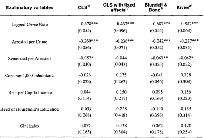
(24) ECONOMIC AND SOCIO-DEMOGRAPHIC DETERMINANTS OF CRIME IN URUGUAY. As mentioned aboye we run the Sargan test to analyze the validity of the instruments. The null hypothesis is that the over-identifying restriction holds. We do not reject the null hypothesis at the 5% levet. We also use the test of serial correlation to study the first and second order residual correlation. In this case, the null hypothesis is that the error term is serially uncorrelated. As expected, we reject the null hypothesis in the first order case since it is serially correlated by construction. But for higher orders we expect no serial correlation and indeed this is our case. At the second order we do not reject the null hypothesis. Therefore, we conclude that the crucial assumption of Arellano and Bond method holds. Table 6 shows the crime regression for the period 1994 to 2006 in which we have data on police forces. The results basically remain as before. The estimated effect of pollee on crime is zero. A main concern with the introduction of cops as explanatory variable is the endogoneity of this variable (Di Tella and Schargrodsky 2004). If the crime rate rises we expect that authorities increase the number of policies to attack crime and therefore we have reverse causality and biased estimators. The Figure 8 plots the evolutions of the crime rate and cops rate. We observe a positive trend in the crime rate but no a clear pattern in the cops rate. This can be explained by a policy decision to do not combat crime with more policemen. In particular, between 1995 and 2006 by law the government could not hire workers. Table 6 Dynamic Panel Data Model for Crime per 1,000 Inhabitants. Variables in logs Explanatory variables. Lagged Crime Rate. OLS with fixed effectsu. OLS". 0.678*** (0.055). Arrested per Crime. -0.260*** (0.056). Sentenced per Arrested. Real per Capita Income. Head of Household's Education. Gini Index. -0.236*** (0.071). -0.052* (0.030). Cops per 1,000 Inhabitants. 0.467*** (0.096). -0.044 (0.043). Blundell & Bond' 0.687*** (0.055) -0.242*** (0.052) -0.063** (0.026). Kiviet2'. 0.582*** (0.068) -0.227*** (0.035) -0.042* (0.022). -0.026. 0.175. -0.041. 0.238. (0.028). (0.263). (0.046). (0.308). 0.044. 0.150. 0.095. 0.156. (0.114). (0.217). (0.169). (0.220). 0.053. -0.228. -0.140. -0.185. (0.268). (0.418). (0.396). (0.314). 0.077. -0.138. 0.062. -0.120. (0.165). (0.304). (0.178). (0.254). 66.

(25) WELL-BEING AND SOCIAL POLICY VOL 6, NUM. 2, pp. 45-73. Table 6 (continued) Explanatory variables. OLS". OLS with Fixed Effects". Blundell & Bond". Kiviet2'. Youth Unemployment (529 years okl). 0.028 (0.026). -0.022 (0.038). 0.038 (0.028). -0.030 (0.053). 1.221***. Urbanization Rate. -2.105. (0.342). 1.232***. (2.754). (0.371). p-value A-B test for AR(1) in first dif. -2.278 (2.311). 0.002. p-value A-B test for AR(2) in first dif. 0.496. p-value Sargan test of overid. restrictions. 0.192. Observations. 228. 228. Sample. 228. 228. 1994 - 2006. Notes: 1/Robust standard errors clustered at the department levet reported in parentheses. 2/Conventional standard errors reported in parentheses. * significant at 10%; ** significant at 5%; *** significant at 1%.. 6.05. 45. 6.00. - 40. 5.95. - 35. 5.90. - 30. 5.85 5.80. - 25. 5.75. 20. 5.70. - 15. 5.65 10. 5.60 5.55. 5. 5.50. o co. o. o o. Cops. o. o o. N. N. — — Crime. Source: National Institute of Statistics (INE).. 67. N. o o. N. Crime per 1,000inhabitants. Cops per 1,000inhabitants. Figure 8 Cops and Crime.

(26) ECONOMIC AND SOCIO-DEMOGRAPHIC DETERMINANTS OF CRIME IN URUGUAY. As estimate previously we can not reject the persistence of crime. The coefficient associated to the lagged crime rate is positive and highly significant. As mention aboye, the Becker's theoretical work assumes a rational behavior of criminals. In this context, crime against the property can be more directly linked with this rationality assumption since this kind of crime could be easily attributable to a rational nature. For this reason, we decided to separately consider crime against person and crime against property. In Table 7 we present the estimations results by type of crime. Table 7 Dynamic Panel Data Model for Crime per 1,000 Inhabitants by Type of Crime. Variables in logs Crime against Person Explanatory Variables. Blundell and Bone. Kiviet2'. Crime against Property Blundell„ and Bond. Kiviety. Lagged Crime Rate. 0.805*** (0.035). 0.760*** (0.046). 0.686*** (0.074). 0.462*** (0.033). Arrested per Crime. -0.082 (0.049). -0.052 (0.055). M.259*** (0.051). -0.244*** (0.027). Sentenced per Arrested. -0.066 (0.041). -0.074 (0.066). -0.077*** (0.025). -0.061* (0.037). Real per Capita Income. 0.126 (0.168). 0.310 (0.322). 0.048 (0.080). -0.002 (0.158). Head of Household's Education. -0.447 (0.430). -0.065 (0.414). 0.026 (0.254). -0.129 (0.215). Gini Index. 0.229 (0.189). 0.183 (0.226). -0.133 (0.119). -0.313** (0.122). Youth Unemployment (529 years old). 0.005 (0.050). -0.078 (0.074). 0.024 (0.025). -0.015 (0.042). Urbanization Rate. 0.187. 0.851. (0.339). (2.038). 1.328*** (0.300). p-value A-B test for AR(1) in first dif. 0.001. 0.004. p-value A-B test for AR(2) in first dif. 0.724. 0.303. p-value Sargan test of overid. restrictions. 0.308. 0.028. Observations. 380. Sample. 380. 380. -1.837** (0.907). 380. 1986 - 2006. Notes: 1 /Robust standard errors clustered at the department level reported in parentheses. 2/Conventional standard errors reported in parentheses. * significant at 10%; ** significant at 5%; *** significant at 1%.. 68.

(27) WELL-BEING AND SOCIAL POLICY VOL 6, NUM. 2, pp. 45-73. The inertia hypothesis holds in both types of crimes and in the case of crime against person the coefficient of the lagged dependent variable has a great magnitude. As expected, the dissuasion variables are only relevant for crime against property. This result has important policy implication. The government can reduce crime with the increase in the police and justice efficiency. Additionally, despite the fact the efforts the government could do in order to reduce crime rate, there will always be a proportion that remain unaffected like homicides, etc. Finally, we go one step further disaggregating crime against person and crime against property in their different typology. We separate crime against the person in aggression and injury, sexual crime, and homicide. Crime against the property was split into theft, rapine, and damage. Table 8 shows the results. Apart from Homicide, we fmd positive and statistically significant crime inertia effects. Overall, dissuasion variables are relevant in crime against property, principally in the case of theft. In addition, it is important to note that some socioeconomic variables like income, education, and youth unemployment affect with the expected sign the rate of sexual crime.. 5. Conclusions We estimated a dynamic panel data model for the Uruguayan departments to analyze the determinants of crime. The results show that a set of economic are not related to crime in general, while socio-demographic variables are indeed related to crime. As socio-demographic variables we consider the urbanization rate and the population density. As we expected these variables positively affects crime. Additionally, we found that an increase in the crime rate tends to perpetuate it overtime and therefore, further research is required to determine the mechanism of perpetuation of crime. It is usually argued that crime rate tend to perpetuate because once an individual is involved in criminal activities there is not backtrack. This point of view could fit in Latin American countries in where prison system collapsed and peer effect in prisons could be representing an important negative extemality. This also encourages human capital depreciation that decreases the cost of crime. In what concern to deterrent factor, they are relevant in the case of crime against property, but not for crime against person. This result has important implications in terms of policies that are aimed to combat crime. The government can reduce crime with more police and a more efficient justice.. 69.

(28) Table 8 Dynamic Panel Data Model for Crime per 1,000 Inhabitants by Type of Crime. Variables in logs Blundell & Bond Crime against Property. Explanatory Variables. Aggression and Injurie. Sexual crime. Homicide. Theft. Rapine. Damage. (0.065). 0.075 (0.087). 0.668*** (0.070). (0.097). 0.659*** (0.098). Arrested per Crime. -0.096* (0.052). -0.007 (0.077). -0.084 (0.092). -0.277*** (0.053). M.208* (0.115). M.188** (0.072). Sentenced per Arrested. -0.081* (0.041). M.095** (0.040). 0.081 (0.113). M.082** (0.029). -0.064 (0.078). -0.027 (0.064). Real per Capita Income. 0.099 (0.169). 0.682*** (0.227). -0.296 (0.476). 0.041 (0.075). 1.191** (0.498). -0.057 (0.295). Head of Household's Education. -0.343 (0.426). M.983* (0.530). -0.936 (1.125). -0.038 (0.246). 0.542 (1.183). 0.479 (0.915). Gini Index. 0.206 (0.200). -0.192 (0.395). 0.904 (0.582). -0.151 (0.110). -0.282 (0.454). -0.103 (0.274). Youth Unemployment (.29 years old). -0.011 (0.051). 0.143** (0.068). -0.092 (0.166). 0.017 (0.024). 0.168 (0.147). 0.074 (0.085). 0.825***. 0.359***. 0.033. 0.391. 3.202. 0.135. (0.332). (0.944). (1.145). (0.328). (2.127). (0.546). p-value A-B test for AR(1) in first dif. 0.001. 0.000. 0.006. 0.005. 0.001. 0.022. p-value A-B test for AR(2) in first dif. 0.464. 0.251. 0.415. 0.512. 0.032. 0.867. p-value Sargan test of overid. restrictions. 0.290. 0.146. 0.107. 0.005. 0.413. 0.906. 380. 380. 380. 380. 380. 380. Urbanization Rate. Observations Sample. 2.231*. 1.536***. 0.437***. 1986 - 2006. Notes: Robust standard errors clustered at the department level reponed in parentheses. * significant at 10%; ** significant at 5%; *** significan at 1%.. ICDETERMINANTS OF CRIME IN U. (0.039). Lagged Crime Rate. 00130-0130S ONV311NONO. Crime against Person. a,.

(29) WELL-BEING AND SOCIAL POLICY VOL 6, NUM. 2, pp. 45-73. Annex Data Sources The variables used in the analysis have an annual frequency at the department level. All variables are available for the 1986 to 2006 period with the exception of cops which is available for the 1994 to 2006 period.. Total Crime Rate: Total crime per 1,000 inhabitants. Source: Statistical Yearbook (Anuario Estadísitco), National Institute of Statistics (Instituto Nacional de Estadística, INE). Cops: Number of policeman combating crime. Source. Ministry of Interior (Ministerio del Interior). Arrested per Crime: Total of arested divided by total crime. Source: Ministry of Interior. Sentenced per Arrested: Total of sentenced divided the total arrested. Source: Ministry of Interior. Unemployment Rate Source: INE. Youth Unemployment Rate: Unemployment rate for individuals between 14 and 29 years old. Source: INE. Real Average per Capita Household Income: Uruguayan pesos of 1997. Source: INE. Population Density: Inhabitants per squared kilometer. Source: INE. Urbanization Rate: Share of population living in urban areas. Source: INE. Border Dummy: Dummy variable that take the value of one in the case of border department with Brazil: Artigas, Cerro Largo, Rivera, and Rocha.. 71.

(30) ECONOMIC AND SOCIO-DEMOGRAPHIC DETERMINANTS OF CRIME IN URUGUAY. References. Di Tella, R. and E. Schargrodsky. "Do Police. Arellano, M. and S. Bond. "Estimation of Dynamic Models with Error Components". Journal of the American Association 76, 1991.. Reduce Crime? Estimates Using the Allocation of Police Forces After a Terrorist Attack". American Economic Review, American Economic Association, vol. 94 no. 1 (March, 2004): 115-133.. Arellano, M. and S. Bover. "Another Look at the Instrumental-Variable Estimator of ErrorComponent". Journal of the American Statistical Association, 1995.. Easterly, W., N. Loayza, and P. Montiel. "Has Latin America's postreform growth been disappointing?" Journal of International Economics, vol. 43 no. 3, 1997.. Becker, G. "Crime and Punishment: An Economic Approach". Journal of Political Economy 76, (1968): 169-217.. Egozcue, M. "Estadísticas sobre los delitos en Uruguay". Mimeo, 1999.. Beck, T., R. Levine, and N. Loayza. "Finance and the Sources of Growth". Journal of Financial Economics, Elsevier, vol. 58 issue 1-2, (2000): 2613 OO.. Eide, E. "Economics of Crime. Deterrance and the. Bertrand, M., E. Duflo, and S. Mullainathan.. A Theoretical and Empirical Investigation". Journal of Political Economy 81, 1973.. Rational Offender". North Holland, 1994.. Ehrlich, I. "Participation in Illegitimate Activities:. "How Much Should We Trust Differences-inDifference Estimates?" The Quarterly Journal of Economics, MIT Press, vol. 119 no. 1 (2004): 249275.. Fajnzylber, P., D. Lederman, and N. Loayza.. Blundell, R. and S. Bond. "Initial Cond tions. Galiani, S. and M. González-Rozada. "Inference. "What Causes Violent Crime?" The World Bank, 1998.. and Moment Restrictions in Dynamic Panel Data Models". Journal of Econometrics 87 (1998): 115143.. and estimation in small sample dynamic panel data models". Mimeo, 2002.. Glaeser, E. and B. Sacerdote. "Why is there More Crime in Cities". NBER Working Paper No. 5430, 1996.. Bruno, G.S.F. "Approximating the Bias of the LSDV Estimator for Dynamic Unbalanced Panel Data Models". Economics Letters 87 (2005): 361366.. Glaeser, E., B. Sacerdote, and J. Scheinkman. "Crime and Social Interactions". Quarterly Journal of Economics 111 (1996): 507-548.. Buonanno, P. and D. Montolio. "Identifying the Socioeconomic Determinants of Crime in Spanish Provinces". Working Paper in Economics No. 138, Universidad de Barcelona. Espai de Recerca en Economia, 2005.. Grogger, J. "Market Wages and Youth Crime". Journal of Labor Economics, University of Chicago Press, vol. 16 no. 4 (October, 1998): 756-91.. Caselli, F., G. Esquivel, and F. Lefort.. Han, L., S. Bandyopadhyay, and S. Bhattacharya. "Determinants of Violent and. "Reopening the Convergence Debate: A New Look at Cross-Country Growth Empirics". Journal of Economic Growth, Springer, vol. 1 no. 3 (1996): 363-89.. Property Crimes in England and Wales: A Panel Data Analysis". Discussion Papers, Department of Economics, University of Birmingham 2010.. 72.

(31) WELL-BEING AND SOCIAL POLICY VOL 6, NUM. 2, pp. 45-73. Jacob, B., L. Lefgren, and E. Moretti. "The Dynamics of Criminal Behavior: Evidence from Wealther Shocks". NBER Working Paper No. 10739, 2004.. Kiviet, J. "On Bias, Inconsistency, and Efficiency of Various Estimators in Dynamic Panel Data Models". Journal of Econometrics 68, (1995): 5378.. Kling, J., J. Ludwing, and E. Katz. "Youth Criminal Behavior In The Moving To Opportunity Experiment". Working Paper No. 6, Princeton University, Department of Economics, Industrial Relations Section, 2004. Leung, S. "Dynamic Deterrence Theory". Economica, London School of Economics and Political Science, vol. 62 no. 245 (1995): 65-87.. S. Raphael and R. Winter. "Identifying the Effect of Unemployment on Crime". Department of Economics, University of California, San Diego, 1998.. Roodman, D. "How to do xtabond2: An introduction to difference and system GMM in Stata". Stata Journal, Stata Corp LP, vol. 9 no. 1 (March, 2009): 86-136. Sah, R. "Social Osmosis and Patterns of Crime". Journal of Political Economy 99 (1991): 12721295.. Vergara, R. "Crime Prevention Programs: Evidence for a Developing Country". Documento de Trabajo No. 362, Department of Economics, Pontificia Universidad Católica de Chile, 2009.. World Bank/Banco Mundial. "El Crimen y la Violencia como problemas para el desarrollo en América Latina y el Caribe". Conference Crimen y Violencia Urbana en Río de Janeiro, Brasil, carried out by the World Bank, 1997.. 73.

(32)