Environmental screening tools for assessment of infrastructure plans based on biodiversity preservation and global warming (PEIT, Spain).

Environmental screening tools for assessment of infrastructure plans based on

biodiversity preservation and global warming (PEIT, Spain)

Luis G. García-Montero , Elena López , Andrés Monzón , Isabel Otero Pastor

Dept. Forest Engineering, E.T.S. Ingenieros de Montes, Technical University of Madrid (UPM), Ciudad Universitaria s/n, Madrid 28040, Spain TRANSyT, E.T.S. Ingenieros de Caminos, Technical University of Madrid (UPM), Avda. Profesor Aranguren s/n, Madrid 28040, Spain

A B S T R A C T

Most Strategic Environmental Assessment (SEA) research has been concerned with SEA as a procedure, and there have been relatively few developments and tests of analytical methodologies. The first stage of the SEA is the 'screening', which is the process whereby a decisión is taken on whether or not SEA is required for a particular programme or plan. The effectiveness of screening and SEA procedures will depend on how well the assessment fits into the planning from the early stages of the decision-making process. However, it is Kevwords- difficult to prepare the environmental screening for an infrastructure plan involving a whole country. To be Environmental screening useful, such methodologies must be fast and simple. We have developed two screening tools which would Strategic environmental assessment make it possible to estímate promptly the overall impact an infrastructure plan might have on biodiversity Infrastructure planning and global warming for a whole country, in order to genérate planning alternatives, and to determine Landscape planning whether or not SEA is required for a particular infrastructure plan.

1. Introduction

The phenomenon of climate change is directly linked to energy consumption and to greenhouse gas (GHG) emissions. At the EU level, the transport sector is the primary driver of the growth in total energy consumption, which is likewise directly linked with total emissions

(EEA, 2006a). Despite the considerable efforts devoted to environmen-tal abatement policies, the high rate of increase in transport demand is outstripping the rate of improvement in environmental technology for transport (Stead, 2001). The result has been a significant increase in greenhouse gas (GHG) emissions from transport, which threatens Europe's progress towards its international commitments, such as the Kyoto targets (UNFCCC, 1997) and the proposals by the EU Council for further emission reductions for developed countries beyond the Kyoto Protocol period (2008-2012) (EC, 2005). The reduction of air pollution is also on the EU agenda, although energy-related emissions (NOx, S02, VOCs) from the transport sector have decreased steadily since 1990

(EEA, 2006b; López, 2007), largely due to the result of increasingly strict emissions standards for the different transport modes, and to fuel switching.

The loss of biodiversity and quality of the environment associated with new transport infrastructure are also concerns for transport policy at the strategic level (EEA, 2006b), as established by the principies of international environmental policy, whose aims are to 'conserve and improve the quality of the environment... based on the precautionary principie' (Articles 6 and 174 of the EU Treaty; Ofiate et al., 2002); and which proposes 'the integration of conservation and sustainable use of biodiversity into the various plans and programmes' (Convention on Biological Diversity 1992, Rio Earth Summit). Treweek et al. (1998)

indícate that infrastructure developments, when considered collective-ly, can be compatible with safeguarding important and protected wildlife habitats and their associated protected species. Norris and Farrar (2001), Brown (2003) and Schumaker et al. (2004) indícate that environmental quality is becoming recognized as a critical factor that should constrain land-use planning, and they also recommend that specialists should adopt approaches in which environmental quality information assists those involved in the development plans.

The Strategic Environmental Assessment (SEA) is one of the best all-round tools for environmental protection, as it permits the concept of sustainability to be integrated into the planning process (Partidario, 2000; Alshuwaikhat, 2005; Chaker et al., 2006). However, the effectiveness of SEA depends on how well the assessment fits into the planning context. Specific procedural steps may improve its effective-ness, but explicit requirements to recognize SEA in decision-making are likely to be a key condition (Dalkmann et al., 2004; Hilden et al., 2004).

stages of a plan and prior to its adoption or to any legal procedures, with the aim of ensuring that SEA is taken into account in the planning process (European Directive 2001/42/EC).

These authors and European Directive indícate that the first stage of a SEA is the screening process. Screening is defined by the European Commission as 'the process by which a decisión is taken on whether or not SEA is required for a particular programme or plan'. The European SEA Directive (EC, 2001) also specifies that screening should be used in the decision-making process to genérate planning alternatives and to contribute to an improvement in the plan itselí

Screening research has made little progress in developing analytical methodologies to resolve technical problems and to incorpórate new findings into the planning process. Von Seht (1999) and Thérivel (2002) point out that it has not been easy to arrive at a methodology for the SEA and screening models. Polichtchouk (1998) indicates that the complex and interdisciplinary nature of environ-mental problems requires the development of a new class of GIS (Geographic Information System), integrating mathematical models, databases and expert knowledge based on a conceptual model.

In light of the scarcity of literature exploring the practical implementation of environmental screening, our paper attempts to contribute to the growing body of knowledge on best practices for this tool. The general objective of the present study is therefore to develop a screening model which would make it possible to estímate promptly the overall impact a Spanish infrastructure plan might have on the environment for the whole Spanish territory (500,000 km2), and to

intégrate this screening into the SEA and decision-making processes. Based on this aim and on previous screening model studies (López, 2007; García-Montero et al., 2008, 2010), our proposal for the environmental screening of infrastructure plans is based on two screening tools for assessment of infrastructure impacts on biodiver-sity preservation and global warming.

2. Methods

2.1. The example of the infrastructure plan: Spanish transport infra-structure plan PEU 2005-2012 guidelines

In December 2004, the Spanish Ministry of Public Works proposed a strategic infrastructure and transport plan known as the PEIT (Ministerio de Fomento, 2004). This document establishes that the priorities in the road transport system for the 2005-2012 period are centred around improving the conditions of service throughout the network with regard to safety and maintenance; streamlining the network by making changes in its structure; completing construction of the high-capacity routes; and the implementation of ITS (Intelligent Transport Systems). Two programmes of actions were set up for this purpose: intercity actions, and the definition of a new basic plan for the high-performance road network (the basic network, with about 15,000 km of infrastructures), which would improve Spain's current road structure. It also includes the termination of the high-capacity routes (> 10,000 vehicles/day), an action plan for long-distance routes, and a programme of construction of urban bypasses, among other projects.

The PEIT's objectives for the railway system are the transformation of this system into the central element of intercity transport services for both passengers and goods. This criterion will make it necessary to concéntrate actions in the corridors in which there is greatest demand, and which have the greatest potential for improving accessibility to the whole of the Spanish territory. The actions will focus on the termination of the high-performance corridors and axes currently under construction, and the modernization of the conven-tional railway network in order to improve goods transportation services by rail, thereby facilitating the exchange between road and sea transport, and enabling interoperability with the French network, among other actions.

2.2. A GIS model for biodiversity and environmental assessment

2.2.1. Step 1: Methodological basis

We selected as the main valuation criteria 'the conservation of biodiversity and the preservation of the environment', and we used the methodology of Ramos (1979) and a GIS model proposed by Mancebo et al. (2005) and García-Montero et al. (2010) (LATINO model). These methodologies are based on models which compare the territorial units in relation to each other, based on the attributes or natural variables in each ofthem.

We looked for biodiversity and environment evaluation criteria based on existing environmental information on a national scale, and used this to draw up the GIS model for biodiversity and environmental assessment in Spain, based on five previous digital maps on a national scale (Table 1). These five maps allowed us to genérate, either directly or by deduction, a set of 12 environmental qualities that represented 12 ráster layers (Table 1). We considered that with these 12 variables it was possible to obtain a basic GIS model for biodiversity and environmental assessment which could be applied rapidly and effectively in the screening of a Spanish infrastructure plan. However, this GIS assessment model is an open system that allows continuous incorporation of new scores.

The GIS software, maps, ráster operations and cartographic formats have been described by García-Montero et al. (2008). The datum and projection was selected according to Eurogeographics' recommendations (EEA, 1999; Geodásie Eurogeographics EUREF, 2006). The precisión threshold was established at 100 m RMS (equivalent to a scale of 1:500,000).

The vector modulus was selected as the method for integrating the different evaluations with numerical vectors. Tran et al. (2006) propose the vector modulus as a useful synthetic valué for integrated environ-mental assessments. Ramos (1979), Martínez-Falero and González (1995), MMA (2000), Mancebo et al. (2005) and García-Montero et al.

Table 1

Twelve environmental variables were used in the GIS model for the assessment of biodiversity in spain (Mancebo et al., 2005; García-Montero et al., 2008).

Environmental variable GIS layers

Biodiversity quality and naturalness associated to the map units Singularity of the map units Naturalness of the map units

Singularity of the map units Habitat sizes of the map units Biodiversity quality and

naturalness associated to the map units Singularity of the map units Biodiversity quality and

naturalness associated to the map units Singularity of the map units Size of the forest units

Total vegetatíon cover (%)

Total forest cover (%)

Digital maps on a national scale

Corine Land Cover 1990 (EEA, 2003)

European Habitats map (DGCN, 2004a)

Spanish Landscape map (MMA, 2004)

Soil map (FAO, 2000)

Spanish Forestry Vegetatíon map

(DGCN, 2004b)

Spanish Forestry Vegetatíon and Corine LC. maps

Method for obtaining the variables and cartographic layers

Panel of experts

Objective classiflcation calculated with SIG Valuation by the experts who generated the original map Objective classiflcation calculated with SIG Panel of experts

Objective classiflcation calculated with SIG Panel of experts

Objective classiflcation calculated with SIG

(2008,2010) also propose the use of the vector modulus in environmental assessment for practical operating reasons. All the normalized variables used as components of the vectors vary between 0 and 1, so to calcúlate each vector modulus, the origin of the coordinates was taken to be {xx xn) with x¡ = 0 (i = 1.... n).

In practice, it is difficult to prepare the screening of an infrastruc-ture plan in a country as large and as diverse as Spain. Therefore, in our study w e have applied the principie proposed by Ramos (1979) and

Otero et al. (1999), who recommend that environmental assessment should focus on the impacts which a priori are seen to be most important. The common premise governing these procedures should be 'to devote the greatest possible effort to the most significant problems', and to apply máximum protection to the áreas with the greatest biodiversity and environment quality.

2.2.2. Step 2: Valuation of variables by means ofrapid consultations with ponéis ofexperts

We consulted a panel of experts in order to obtain a set of four biodiversity and environmental valuation qualities to represent four ráster layers (Table 1), according to the following procedures:

I. The biodiversity and naturalness associated to the units in the Corine Land Cover 1990 map (EEA, 2003) was based on the hierarchical classifications proposed by the Corine Project, and interpreted by four experts in vegetation and land-use at the School of Forestry in Madrid.

II. A map of naturalness of the units in the European Habitats map

(DGCN, 2004a) was generated by obtaining a ráster layer from an original vector map using a field containing a naturalness valué (1 to 3) for each polygon on the map. These naturalness valúes were previously assigned by the experts who partici-pated in the original vector map of the European Habitat Project. III. The biodiversity and naturalness associated to the units in the Spanish Landscape map (MMA, 2004) were assessed using the legend, and interpreted by four experts at the School of Forestry in Madrid, based on the previous landscape research experience of this group (Otero Pastor et al., 2007).

IV. The biodiversity and naturalness associated to the units in the Soil map (FAO, 2000) was assessed using the legend, and then evaluating as a whole the productive capacity, biodiversity, naturalness and uniqueness of the soils in Spain. This was done following the FAO's hierarchical classifications of soil taxono-my, and interpreted by a panel of five experts from the Soil Sciences Department at the Complutense University in Madrid.

2.2.3. Step 3: Objective assessment of the vegetation by analysis of its cover

An objective assessment was made of the vegetation cover expressed as a percentage of the vertical extensión of the vegetation formations (Table 1), following two procedures:

I. The percentage of total vegetation cover (% extensión of vertical vegetation shading) was evaluated on a national scale. This was done using the data from the Spanish Forestry Vegetation map (DGCN, 2004b). In the áreas for which no information was available, the Corine Land Cover map was used; its legend provides an estímate of the mínimum and máximum vegetation cover for the different units, and an average valué was assigned for the cover for each of these units. II. The percentage of total forest cover (% extensión of vertical tree canopy shading) was assessed on a national scale, following the procedure described above. To define the category of 'forests', we followed the criteria used in both maps, which take the mínimum threshold to be 30% cover by trees of over 5 m in height.

2.2.4. Step 4: Objective assessment of territorial singularity

In order to safeguard biodiversity, w e assessed the territorial singularity of the different categories or classes in the Habitats, Corine

Land Cover, Landscape and Soil maps (Table 1). This was done using an objective classification of their units calculated with the SIG. The following index of singularity was applied (Ramos, 1979; MMA2000):

where S = territorial singularity index; Max = Ha. of the map's largest category; Min = Ha. of the map's smallest category; and x = Ha. of the map category being evaluated.

Singularity was assessed on a logarithmic scale. This transformation made it possible to maximize the valué of the categories with smaller áreas, and also to obtain a scale with fewer units. Thus the category with the greatest surface área was awarded the lowest singularity valué (0) and the category with the least surface área was awarded the máximum valué (4.62). This continuous scale was then transformed into a discrete scale of five classes, which were obtained by rounding each decimal valué up to the next whole number. We thus obtained a higher singularity valué for the least represented classes in the territory, in order to safeguard biodiversity.

In the case of the Corine Land Cover map, we carried out a double singularity analysis. First w e estimated the singularity relating to Spain, which constitutes the main singularity scale. This scale was then refined by making a second calculation of singularity using the Corine Land Cover map for the whole of Europe. This increased the singularity valué for those categories whose presence in Europe is concentrated in the Iberian Península (over 40%), as well as for those categories of Corine Land Cover which are very scarce in Europe as a whole, regardless of their abundance in Spain.

2.2.5. Step 5: Objective assessment of habitat sizes

Gontier et al. (2006) indícate that habitat loss is a major threat to biodiversity. Environmental impact assessment and strategic envi-ronmental assessment are essential instruments used in physical planning to address such problems. Yet there are no well-developed methods for quantifying and predicting impacts on habitat loss. These authors also highlight the gap existing between research in GIS-based ecological modelling and current practice in biodiversity assessment within environmental assessment.

We evaluated the habitat sizes of the different categories or classes in the Habitats map, and of the polygons with forest cover (identified with the Spanish Forestry and Corine Land Cover maps) (Table 1). This was done using an objective classification of their units calculated with the SIG The following procedure was used (Ramos, 1979; MMA, 2000):

I. We calculated the surface área of each of the polygons on these maps in order to give a positive valuation to those with a greater surface área for each category or class, so as to provide more protection for the most representative polygons in each class and to favour the conservation of natural áreas.

II. The valuation was done by assigning a scale of four discrete valúes which correspond to each of the four percentiles of the numeric distribution of frequencies of surface sizes:

H.a. Habitat size class 1 = sizes of polygons corresponding to the first percentile (0-25%) of the distribution of frequencies of sizes.

H.b. Habitat size class 2 = sizes of polygons corresponding to the second percentile (25-50%).

II.c. Habitat size class 3 = sizes of polygons corresponding to the third percentile (50-75%).

Il.d. Habitat size class 4 = sizes of polygons corresponding to the fourth percentile (75-100%).

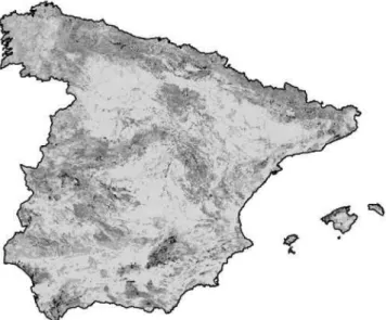
Fig. 1. GIS model for biodiversity and environmental assessment for the whole of Spain.

Metadata: European projection standard Lambert Equal Área and Datum ETRS89.100 m pixel-raster maps. Model scale: 1:500,000. Colour codes: classes of natural quality 1 and 2 = light grey; class of natural quality 3 = grey; class of natural quality 4 = dark grey; class of natural quality 5 = black.

2.2.6. Step 6: Normalization of the 12 variables

The 12 variables were then normalized to avoid overlapping during their subsequent integration into the model. Normalization consisted of changing the original valuation scale for each variable, which was transformed into a common final continuous scale from 0 to 1 for all the variables. This was done by means of an equation applied to the original discrete scales and another equation applied to the original continuous scales (Mancebo et al., 2005). The following formula was used to convert the discrete scales into a continuous scale from 0 to 1:

Xn 0.5

Max (2)

The following equation was used to transform a continuous scale into another normalized continuous scale from 0 to 1:

Xn / x - Min

{Max - Min (3)

2.2.7. Step 7: Integration ofthe 12 variables into the model The 12 normalized ráster variables were integrated using GIS combine operations. Each pixel of 1 ha of territory was assigned a vector with the 12 natural variables valued. We obtained n vectors distributed among the 50 million 1-ha pixels in Spain.

The next step was to order the n vectors using the modulus or Euclidean distance, to assign a synthetic valué oftheoretical biodiversity and environmental quality. The vector was used to order the n vectors obtained based on their components, and:

v\2 1...12 (4)

where v is the vector modulus; and v¡ is a vector component. A total of 102,240 different vectors were obtained with 12 components, assigned to each of the 50 million 1 -ha grid squares for Spain. Then the valúes obtained for each of the n Euclidean distances were normalized into five equivalent classes, corresponding to the five types oftheoretical biodiversity and environmental quality (1 to 5). This normalized classification was obtained by applying the following formula:

Biodiversity quality class = «V - vMin) / (vMtK - vMin))*(5 + 0.5) (5)

where v is the vector modulus of each ofthe n vectors obtained; vMin

is the mínimum vector modulus obtained; vMax is the máximum

vector modulus obtained; the very low biodiversity and environmen-tal quality class is obtained when 0.5 < v < 1.5; low quality class when 1.5<v<2.5; modérate quality class when 2.5<v<3.5; high quality class when 3.5 < v<4.5; and very high quality class when 4.5 < v< 5.5.

Table 2

Checklist and synthetic environmental impact valúes based in García-Montero et al. (2008) to estímate the relative impact of 27 types of infrastructure construction project on the local environment (Impact class 0 = compatible; Impact class 1 = modérate; Impact class 2 = severe; Impact class 3 = critical).

27 types of construction project New roads: urban highways New roads: type-III regional highways New roads: type-II regional highways New roads: type-I regional highways New roads: national A-roads New roads: dual carriageways New roads: motorways New conventional train New high-speed train (AVE) Urban highway to dual carriageway Urban highway to motorway

Regional highway-III to regional highway-II Regional highway-III to regional highway-I Regional highway-III to national A road Regional highway-III to dual carriageway Regional highway-III to motorway Regional highway-II to regional highway-I Regional highway-II to national A road Regional highway-II to dual carriageway Regional highway-II to motorway Regional highway-I to national A road Regional highway-I to dual carriageway Regional highway-I to motorway National A road to dual carriageway National A road to motorway Dual carriageway to motorway Conventional train to AVE

Table 3

Synthetic environmental impact of 27 types of construction project (based in García-Montero etal., 2008).

27 types of construction project Dual carriageway to motorway

Regional highway-III to regional highway-II Regional highway-II to regional highway-I Regional highway-II to national A road New roads: urban highways Urban highway to dual carriageway Urban highway to motorway Regional highway-I to national A road Regional highway-III to regional highway-I Regional highway-III to national A road New roads: type-III regional highways New conventional train

Conventional train to AVE New roads: type-II regional highways National A road to dual carriageway National A road to motorway Regional highway-I to dual carriageway New roads: type-I regional highways Regional highway-I to motorway Regional highway-II to dual carriageway Regional highway-III to dual carriageway New roads: national A-roads

Regional highway-II to motorway New high-speed train (AVE) Regional highway-III to motorway New roads: dual carriageways New roads: motorways

Vector module 2.1 3.0 3.8 3.8 4.0 4.4 4.4 4.4 4.8 4.8 6.1 6.4 6.6 6.6 7.5 7.8 7.9 7.9 8.2 8.3 8.4 8.7 8.7 8.8 8.9 9.8 9.8 Normalization 0.5 1.0 1.4 1.4 1.5 1.7 1.7 1.7 1.9 1.9 2.6 2.7 2.8 2.8 3.3 3.5 3.5 3.5 3.7 3.7 3.8 3.9 4.0 4.1 4.1 4.5 4.5

Máximum level of potential impact <1.5) <1.5) <1.5) <1.5) 1.5-2.5) 1.5-2.5) 1.5-2.5) 1.5-2.5) 1.5-2.5) 1.5-2.5) 2.5-4.0) 2.5-4.0) 2.5-4.0) 2.5-4.0) 2.5-4.0) 2.5-4.0) 2.5-4.0) 2.5-4.0) 2.5-4.0) 2.5-4.0) 2.5-4.0) 2.5-4.0) 2.5-4.0) >4) >4) >4) >4)

Potential impact codes 1 1 1 1 2 2 2 2 2 2 3 3 3 3 3 3 3 3 3 3 3 3 3 4 4 4 4 Impact types Compatible Compatible Compatible Compatible Modérate Modérate Modérate Modérate Modérate Modérate Severe Severe Severe Severe Severe Severe Severe Severe Severe Severe Severe Severe Severe Critical Critical Critical Critical The 27 vector modules were calculated and normalized, to assign each of the 27 construction projects a synthetic valué of potential impact in four equivalent classes (Impact class 1 : compatible; Impact class 2 = modérate; Impact class 3 = severe; Impact class 4 = critical).

Normalization = [(x — Min/Max — Min) x4)] + 0.5.

García-Montero et al. (2010) have proposed 100 classes of environmental quality in the Spanish territory based in the LATINO model (LArge Territory Integrated eNvirOnmental model). However, in the present study, the use of five classes of biodiversity and

environ-mental quality is sufficient for a screening, as this is a preliminary classification which clearly distinguishes extreme cases of high and low biodiversity and environmental quality of a territory on a nationwide scale.

Table 4

Model of a double-entry evaluation matrix integra ting the 5 classes of biodiversity quality (1 = very low, 2 = low, 3 = average, 4 = high, 5 = very high) with the 4 synthetic valué of potential environmental impact levéis (1 = compatible; 2 = modérate; 3 = severe; 4 = critical) for the 27 construction projects (12-km bands) based in García-Montero et al. (2008).

27 types of construction project Dual carriageway to motorway

Regional highway-III to regional highway-II Regional highway-II to regional highway-I Regional highway-II to national A road New roads: urban highways Urban highway to dual carriageway Urban highway to motorway Regional highway-I to national A road Regional highway-III to regional highway-I Regional highway-III to national A road New roads: type-III regional highways New conventional train

Conventional train to AVE New roads: type-II regional highways National A road to dual carriageway National A road to motorway Regional highway-I to dual carriageway New roads: type-I regional highways Regional highway-I to motorway Regional highway-II to dual carriageway Regional highway-III to dual carriageway New roads: national A-roads

Regional highway-II to motorway New high-speed train (AVE) Regional highway-III to motorway New roads: dual carriageways New roads: motorways

Potential impact codes 1 1 1 1 2 2 2 2 2 2 3 3 3 3 3 3 3 3 3 3 3 3 3 4 4 4 4

riass quality 1 Class quality 2 1 1 1 1 1 1 1 1 1 1 2 2 2 2 2 2 2 2 2 2 2 2 2 3 3 3 3

Class quality 3 1 1 1 1 2 2 2 2 2 2 3 3 3 3 3 3 3 3 3 3 3 3 3 4 4 4 4

Class quality 4 2 2 2 2 3 3 3 3 3 3 4 4 4 4 4 4 4 4 4 4 4 4 4 4 4 4 4

Table 5

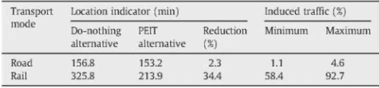
Travel-time savings and estimated induced traffk. Transport

mode

Road Rail

Location indicator (min) Do-nothing

alternative 156.8 325.8

PEIT alternative 153.2 213.9

Reduction

(%)

2.3 34.4

Induced traffk (%) Mínimum

1.1 58.4

Máximum

4.6 92.7

Table 6

GIS ráster model for biodiversity and environmental assessment. Natural quality

Quality class 1 Quality class 2 Quality class 3 Quality class 4 Quality class 5

class Extensions of 9,110,329 14,962,451 15,522,632 9,673,891 588,741

territory (ha) Extensions of territory (%) 18.3

30.0 31.1 19.4 1.2

This model classifles the Spanish territory into 5 classes of biodiversity and environmental quality (Mancebo et al., 2005; García-Montero et al., 2010).

2.3. First screening tool for assessing the impact of the PEIT on Spanish biodiversity and environment

2.3.1. Step I: ¡ntegration with the infrastructures map

We established which zones would be most directly affected by the roads and railway lines in the PEIT 2005-2012. This operation was done by means of an analysis with the GIS, in which the scenario ofthe linear infrastructures existing in 2005 (scenario 0) was compared to the linear infrastructures planned for 2012. Then we defined and mapped 12-km-wide corridors or potential impact bands around each ofthe new infrastructures in the PEIT (2 km to compénsate for lack of map definition, and 10 km of territory potentially affected by each infrastructure). These corridors represent áreas with a high risk of environmental impact caused by the PEIT (Fig. 1). Five-km ( + 1) bands were selected at each side of the routes planned in the PEIT, based on a comparison with other environmental impact studies for several linear infrastructure projects (Ramos, 1979; Otero etal., 1999; MMA, 2000; García-Montero et al., 2008). Moreover, we have repeated the same GIS screening models using 24-km-wide corridors or potential impact bands around each of the new infrastructures in the PEIT, to compare 12-km versus 24-km-wide corridors. The future environmental impact in these corridors was assumed to be uniform across the whole width of the band.

Within the 12-km corridors around the infrastructures, we located and represented the five classes of biodiversity and environmental quality of the territory shown on the 1:500,000 map of Spain. This ¡ntegration generated a ráster map with the biodiversity and environmental quality valúes of the áreas which are potentially affected by the new roads and railways planned in the PEIT.

Fig. 2. Potential impact map: result of screening model for assessing the impact of PEIT infrastructures on Spanish biodiversity and environment (only 12-km-wide corridors around each ofthe new infrastructures in the plan are defined and mapped). Metadata: European projection standard Lambert Equal Área and Datum ETRS89.100 m pixel-raster maps. Colour codes: compatible potential impact = light grey; modérate potential impact = grey; severe potential impact = dark grey; critical potential impact = black

2.3.2. Step 2: Creation of a rapid checldist of the synthetic potential environmental impact of the construction projects planned

We identified 27 types of construction project in the PEIT 2005-2012. We have created a checklist to estímate their potential environmental impact (with valúes of between 0 and 3) based in García-Montero et al. (2008) (Table 2). This checklist was drawnupby consulting 10 expert researchers on transport subjects (panel of experts) from the Transport Research Centre TRANSyT at the Technical University of Madrid (UPM) and the Complutense University of Madrid. The checklist was made using the vector modulus and Analytical Hierarchy (Saaty, 1980) by lining up each ofthe 27 types of construction project or alternatives planned in the PEIT with each of the elements in the local environment listed in SEA European Directive 2001/42/EC(Table3).

2.3.3. Step 3: ¡ntegration ofthe synthetic potential environmental impact checklist in the biodiversity and environmental quality for the 12-km corridors around the infrastructures

The last step in this first screening model was to intégrate the five classes of biodiversity and environmental quality (very low, low, average, high, very high) mapped in the 12-km corridors around the infra-structures with the four synthetic potential environmental impact levéis (1 to 4) for the 27 construction projects in the checklist. This ¡ntegration was done using as a model a double-entry evaluation matrix based on

Table 7

Extensions of Spanish territory which may be affected by the PEIT 2005-2012 plan, with the different degrees of potential environmental impact using 12-km versus 24-km-wide corridors around each of the new infrastructures in the PEIT

Environmental impact class

Compatible potential impact Modérate potential impact Severe potential impact Critical potential impact

Total extensión (ha) potentially affected using 12-km-wide corridors 3,256,811 3,928,807 3,923,072 2,921,801

Relative % of área within the áreas potentially affected using 12-km-wide corridors

23.2 28.0 28.0 20.8

Total extensión (ha) potentially affected using 24-km-wide corridors 5,471,659 6,781,293 6,978,923 5,377,177

Relative % of área within the áreas potentially affected using 24-km-wide corridors

García-Montero et al. (2008) (Table 4), which was applied only in the 12-km bands around the infrastructures. The criteria applied in this evaluation matrix were the optimization of the máximum protection of the pixels in the territory (1 ha) with the greatest biodiversity and environmental quality and the lowest incidence in Spanish territory; as opposed to the lower protection of the pixels with less biodiversity and environmental quality and greater frequency. These criteria are connected to those of Treweek et al. (1998), Brown (2003) and Schumaker et al. (2004). This evaluation matrix allowed us to propose as a final result four potential impact classes of the PEIT 2000-2007 on biodiversity and environment (1 = compatible; 2 = modérate; 3 = severe; 4 = critical) (Table 4) within these 12-km bands.

2.4. Second screening toolfor assessing the impact of the PEIT on global warming

2.4.1. Step I: Travel demand forecasts

López (2007) indicated that a national transport model is not available in Spain to date, although its development is currently on the Spanish research agenda (ETT and EPYPSA, 2006). This fact made it difficult to calcúlate the total C02 emissions in each alternative of an

infrastructure plan. Therefore, a simplification has been made in order to obtain an approximate valué of these emissions.

It is well reported that induced travel is an important component of travel demand (Goodwin, 1996; Guirao, 2000; Cervero and Hansen, 2002; Lee, 2002; Litman, 2004). With improved transportation condi-tions, short-term effects (e.g., route switches, mode switches, changes of destination, and new trip generation) and long-term effects (e.g., change in household car ownership, and spatial reallocation of activities) will be observed.

Many studies have estimated travel-time elasticities - mostly related to highway expansions -, but one of the difficulties in interpreting these results is the uncertainty of the time frame that is applicable to the data (Lee, 2002). The valué of the elasticity of the transport demand is obtained by calculating the percentage by which travel demand varies when another variable (normally travel time) varies by 1% (López, 2007). Goodwin (1996), Noland and Lem (2002) and Cervero and Hansen (2002) provide reviews of many empirical studies on induced demand due to road capacity expansions. For example, Goodwin (1996) found that proportional savings in travel time were matched by proportional increases in traffic on almost a one-to-one basis. Other works suggest an average valué for the elasticity of travel volume with respect to travel time of about — 0.5 to — 1.0 in the short term (these valúes signify that a 1% increase in travel time translates into a 0.5-1.0% reduction in demand), and up to - 2 . 0 in the long term (Lee, 2002).

Rail-related studies are less common. They mostly agree that demand for rail services is much more sensitive to changes in cost and travel time than the demand for automobile travel. Morrison and Winston (1985) found that rail demand is elastic with respect to time, estimating it as —1.67 for business trips and —1.58 in vacation trips. Bel (1997) carried out a study with Spanish data and estimated rail travel-time elasticities of —2.66 (for daytime traffic trains below 400 km) and — 2.37 for trips over 400 km. Other works of intercity

Table 9

Forecast induced traffic and corresponding increases in GHG emissions: do-nothing vs. PEIT alternative (road and rail modes); TREMOVE 2.44 MODEL (Transport & Mobility Leuven and K.U. Leuven, 2006).

Traffic (million vkm)

GHG emissions

(tco2)

Increase in GHG emissions

Do-nothing alternative PEIT alternative

Do-nothing alternative PEIT alternative

Absolute (t C02)

Relative3 (%)

Global relativeb (%)

Mínimum Máximum Mean

Mínimum Máximum Mean Mínimum Máximum Mean Mínimum Máximum Mean Mínimum Máximum Mean

Road 332,359 336,082 347,714 340,037 72,513,766 73,279,001 75,670,365 74,474,684 765,235 3,156,599 1,960,918 1.0 4.4 2.7 1.0 4.3 2.7

Rail 275 436 531 370 234,275 365,756 442,987 404,371 131,481 208,712 170,096 56.1 89.0 72.6 0.2 0.3 0.2 Percentage change of each mode's emissions of the do-nothing alternative. Percentage change of total road and rail emissions of the do-nothing alternative.

HSR projects planned in Japan, computing short term induced travel elasticities, are presented by Yao and Morikawa (2005). In summary, for the rail mode 'across all relations, account being taken of the weight of each relation, an approximate travel-time elasticity of — 2.2 emerges' (Savelberg and Vogelaar, 1987).

To compénsate for this uncertainty in forecasts of travel demand, rather than taking a single valué for travel-time elasticities, a range of — 0.5 to —2.0 will be used for the road mode, and —1.7 to —2.7 for the rail mode.

2.4.2. Step 2: Calculation of travel-time savings

The approach used to compute travel-time savings is based on the calculation of accessibility indicators. The selected formulation is that of the location accessibility indicator, a 'travel cost indicator' (López, 2007), which computes average travel time to the set of destinations. This indicator was previously used in similar studies at the Spanish national level (Monzón et al., 2005). The formulation chosen is included in Eq. (6).

£

The location indicator (L¡) was computed as the average travel time (in minutes) to the set of destinations, using the population of each destination as the weighting variable.

The set of destinations includes locations in Portugal and the three southern regions of France. The location indicator is therefore used as a proxy for the evaluation of travel-time savings, when its results in the PEIT 2005-2012 alternative are compared to those of the

do-Table S

Extensions of Spanish territory which may be affected by the plans PIT 2000-2007 (García-Montero et al., 2008) and PEIT 2005-2012, with the different degrees of potential environmental impact (using 12-km-wide corridors around each of the new infrastructures).

Environmental impact class

Compatible potential impact Modérate potential impact Severe potential impact Critical potential impact

Total extensión (ha) potentially affected by the PIT 2000-3,549,288 4,955,127 1,892,566 3,517,960

-2007

Relative % of área within the áreas potentially affected by the PIT 2000-2007 25.5

35.6 13.6 25.3

Total extensión (ha) potentially affected by the PEIT 2005-3,256,811 3,928,807 3,923,072 2,921,801

2012

Relative % of área within the áreas potentially affected by the PEIT 2005-2012 23.2

nothing alternative. Henee, a single aggregated valué of the location indicator for all Spain has been computed and compared to that ofthe do-nothing alternative. The calculation, in percentage changes, has been translated into the corresponding increases in travel demand by using the range of travel-time elasticities cited above (Table 5).

2.4.3. Step 3: Computation ofthe global warming performance indicator The next step in the second screening tool (GHG emissions screening tool) is the calculation ofthe performance indicator, which consists of transforming the estimated increase in travel demand into the corresponding increase in GHG emissions. This estimation was done with versión 2.44 ofthe TREMOVE model (Transport & Mobility Leuven and K.U. Leuven, 2006). TREMOVE is a policy assessment model designed to study the effeets of different transport and environment policies on transport sector emissions.

The model estimates the transport demand, the modal split, the vehicle fleets, the emissions of air pollutants and the welfare level under different policy scenarios. All relevant transport modes are modelled. TREMOVE models both passenger and freight transport, and covers the period 1995-2020. TREMOVE consists of 21 parallel country models. Each country model consists of three inter-linked 'core' modules: a

transport demand module, a vehicle turnover module and an emission and fuel consumption module, to which a welfare cost module and a well-to-tank emissions module is added. This model was developed by Transport & Mobility Leuven and the K.U. Leuven in a service contract for the European Commission, DG Environment (http:// www.tremove.org). Model runs were carried out with the data on induced traffic, resulting in the corresponding C02 emissions.

3. Results and conclusions

The GIS model for biodiversity and environmental assessment classifies the Spanish territory into the 5 classes of biodiversity and environmental quality shown in Table 6 and Fig. 1 (Mancebo et al., 2005; García-Montero et al., 2010). The application of distribution frequencies for each of the quality classes appears to be a suitable approach for use in developing an infrastructure plan, and for incorporating the map of biodiversity and environmental quality into its planning procedures. This model shows that the planning of infrastructures would be permitted in 48.3% of Spanish territory (Table 6), as this would affect grid squares with low quality valúes (classes 1 and 2). However the planning of infrastructures could not

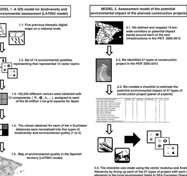
MODEL 1. A GIS model for biodiversity and environmental assessment (LATINO model)

MODEL 2. Assessment model of the potential environmental impact o f t h e planned construction projects

1.1. Five previous thematic digital maps on a naüonal scale

|±J"T1

4

1.2. Set of 12 environmental qualities representing that represented 12 ráster layers

1.3.102,240 different vectors were obtained with 12 components ( Vk', O , 4,...),assigned to each

of the 50 million 1-ha grid squares for Spain

%

2.1. We defined and mapped 12-km-wide corridors or potential impact bands a round each of the new infrastructures in the PEIT 2005-2012

2.2. We identified 27 types of construction project in the PEIT 2005-2012

2.3. We created a checklist to estimate the potential environmental Impact of 27 types of construction project (panel of experts)

4

H

4

• , : • • : • =

N d » r o a « New r c a d i

Htm r o i d ;

N*IY roaas

New reato

.... ,,...

.

'»•:?•! lee. ^r3 l tkjnways t y p é ' l l f e ^ i m j Inij'".'.;iyi [fpo-l regional hijjhnvjy¿ ríatofWJ A-IOMS dual camageways motoivays

Ge-uto gy So¡ 5 0 2 2

2 2

3 3 3 3

3 a

3 3

< • - < • •

D

2 2 3

3 3

•=-•:;¡r hyd'ogeolrjgy 0 ? 2

:<

-j :•

v =

2 0

: ; i •;-..!,.! 0 L'

?

•>

3

3 S

H e * tigti-spaed Main [AVE| U i b a r h i g h w a y t o dual caí luijaivay Urtvkii r t g r w a y to rnotorw j y •!••; y ; . ; ••.;; -v.,•!-.••• •:• ¡í íniíiM l i : , ; - . o y l l

1.4. The valúes obtained for each of the n Euclidean distan ees were normalizad into five types of biodiversity and environmental quality (1 to 5)

1.5. Map of environmental quality in the Spanish territory (LATINO model)

\p~--^

2.4. The checklist was made using the vector modulus and Analytical Hierarchy by lining up each of the 27 types of project with each of the elements in the local environment listed in SEA European Directive

be sited in 20.6% of the territory, as this would affect grid squares with high valúes (4 and 5) (Table 6).

The first GIS screening tool, for assessing the impact of the PE1T on Spanish biodiversity and environment, shows that the PE1T would potentially affect at least 28.1% of Spanish territory, that is to say a total of 14,030,491 ha. Such a great expanse is due to the large number of infrastructures planned. Table 7 and Fig. 2 show the expanses of Spanish territory which may be affected by the Plan, with different degrees of potential environmental impact (within the 12-km corridors around the planned infrastructures).

The first effect that the GIS screening tool had on the planning processes of the plan was to show the high environmental risk represented by the initial PE1T proposal it contained. The first screening tool showed that at least 20.8% of the áreas affected by the PE1T are subject to a high risk of 'potential critical impact' (Table 7). This means that the future Environmental Impact Assessment (E1A) procedures applied to each specific road and railway project in this infrastructure plan, in the áreas indicated as 'critical' in the screening, have a high likelihood of obtaining a negative E1A declaration from the independent environmental body, which will compromise the legal feasibility of these particular projects.

The results of the GIS screening tool also highlighted other environmental errors in the design of the infrastructure plan we used as a sample case. A comparison of the different percentages of territory in the five natural quality classes in Spain with the percentages of the four classes of potential impact of the PE1T obtained for the 12-km corridors reveáis several problems:

I.- The áreas which obtained an assessment of 'very low and tow' biodiversity and environmental quality (classes 1 and 2) account for 48.3% of the Spanish territory, that is, 24,072,780 ha (Fig. 1, Table 6). Spain has large expanses of territory whose natural environment has been drastically altered, a fact which can be

explained by the Iberian Peninsula's long history of human intervention. However, the PE1T planning process has not taken advantage of these áreas for routing new infrastructures. II.- This has meant that the áreas affected by the PEIT (12-km

corridors) which present compatible potential impacts (class 1) only account for 23.2% of the total environmental impact. This valué is clearly less than the affected áreas which have a 'modérate' potential impact (class 2), representing 28.0% of the affected territory, and zones with 'severe and critical' potential impacts (classes 3 and 4), which represent 48.8%.

Table 7 shows the comparison of the GIS screening results using 12-km versus 24-12-km-wide corridors or potential impact bands around each of the new infrastructures in the PEIT. The relative % of the área within the potentially affected áreas in the case of the 12-km-wide corridors is very similar to in the 24-km corridors. These results confirm that 12-km-wide corridors would be significant in the proposed GIS screening models, based on the scale and level of detail used.

This first screening diagnosis leads to the conclusión that the PEIT should be unequivocally subjected to a SEA procedure, and that the results of the GIS screening tool should be taken into account in the infrastructure planning process. Moreover, the GIS screening tool generated two digital maps for this plan (Figs. 1 and 2) which allowed us to lócate other corridors which could more easily accommodate some new and alternative routes in a revised and improved PEIT.

A previous GIS screening tool versión was applied to an earlier Spanish infrastructure plan known as PIT 2000-2007 (within the 12-km corridors around the planned infrastructures) (García-Montero et al., 2005, 2008). The Spanish Ministry of Public Works has used the GIS screening results applied to PIT 2000-2007 to improve the current infrastructure plan known as PEIT 2005-2012 (Ministerio de Fomento, 2003,2004). Table 8 demonstrates how the GIS screening tool applied

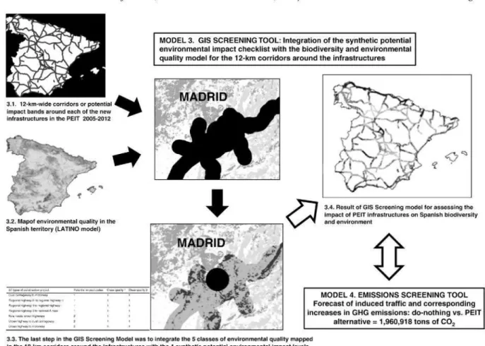
MODEL 3. GIS SCREENING TOOL: Integration of the synthetic potential environmental impact checklist with the biodiversity and environmental quality model for the 12-km corridors around the infrastructures

3.1. 12-km-wide corridors or potential impact bands around each of the new infrastructures inthe PEIT 2005-2012

<©"»

3.2. Mapof environmental quality in the Spanish territory (LATINO model)

=.pH':"•'"-" ly-rrf-lí

MWVB'llO H-V1--JV

3-4. Result of GIS Screening model fora&seosingthe impact of PEIT infrastructures an Spanish biodiversity

and environment

0

MODEL 4. EMISSIONS SCREENING TOOL Forecast of induced traffic and corresponding increases in GHG emissions: do-nothing vs. PEIT

alternative = 1,960,918 tons of C 02

3.3. The last step in the GIS Screening Model vuas to intégrate the 5 classes of environmental quality mappcc in the 12-km corridors around the infrastructures with the 4 synthetic pDlential environmental impact levéis

(1 to 4) for the 27 cortstruction projects in the checklist. This integration was done using as a model a

double-entry evaluation matrix.

to PEIT 2005-2012 shows a smaller critical potential impact for PEIT 2005-2012 (20.8%) than PIT 2000-2007 (25.3%). This comparison therefore proves that the integration of the GIS screening results to genérate planning alternatives is a useful mechanism for improving the importance of biodiversity and environmental quality in the decision-making process.

The results of the second screening tool for assessing the impact of the PEIT on global warming are summarized in Table 9. The do-nothing alternative in the road mode accounts for over 72.5 million tons of C02. It can be seen how the mean increase in GHG emissions

due to the extensión of the HCR network included in the PEIT accounts for nearly 2 million tons of C02, which represents a 2.7% increase

compared to both the do-nothing alternative valué for the road mode. On the other hand, the do-nothing alternative in the rail mode accounts for only 234,000 tons. The extensión of the HSR network included in the PEIT accounts for nearly 170,000 tons of C02, which

represents an increase of over 72%, in terms of the do-nothing alternative valué for the rail mode, whereas it represents only a 0.2% increase in total road and rail emissions in the do-nothing alternative. The comparison of the absolute increases in GHG emissions between road and rail modes (2 million vs. 170,000 tons of C02) gives an idea of

the significant difference in the contribution of the above transport modes to GHG emissions, which is obviously proportional to their corresponding traffic volumes. In any case, the results of the second screening tool for assessing the impact of the PEIT on global warming confirmed the conclusión that the plan should be subjected to a SEA procedure, and showed also that the increases in GHG emissions should be taken into account in the PEIT planning process.

The methodology and selection of both tools does not enable us to determine where the most significant environmental problems are to be found. It provides us with a tool to ascertain the possible impact of a planning alternative on biodiversity and climate change. Other environmental impacts are not within the scope of this article.

In summary, we propose two screening tools whose methodolo-gies are designed to be fast and simple. In Figs. 3 and 4 we have included some Dow charts of all the steps involved in these screening tools. The environmental imbalances detected in the planning processes for the initial PEIT 2005-2012 plan in our study reveal that the planning process did not include enough environmental criteria or models. Therefore, it is very important that the two screening tools and the SEA should be integrated into the planning processes, as this will reduce the time and cost needed for the preparation of the infrastructure plan, improve their quality and reliability, and encourage public participation. It will therefore contribute to better and more transparent environmental decision-making, thus promoting sustainable development.

Acknowledgments

We would like to thank all the personnel at TRANSyT (UPM), Department of Soil Science at the Complutense University, S. Mancebo, M.A. Casermeiro, Margarita, Luis, Pablo and Miriam, for their support. We thank the Centro Geográfico del Ejército and authorities at the Ministerio de Defensa of Spain. The research dealt with in this article forms part of the Projects entitled "Análisis de los impactos territoriales producidos por los modos de transporte terrestres definidos en el Plan de infraestructuras 2002-2007 C03043002" (Ministerio de Fomento, granted in 2003) and "Evaluación de los efectos del Plan de infraestructuras 2000-2007 sobre la movilidad, el territorio y la socioeconomía en el contexto de la U.E. ampliada" (CyCLT, granted in 2004).

References

Alshuwaikhat HM. Strategic environmental assessment can help solve environmental impact assessment failures in developing countries. Environ Impac Assess Rev 2005;25:307-17.

Bel G. Changes in travel time across modes and its impact on the demand for inter-urban rail travel. Transport Res-E 1997;33:43-52.

Brown AL. Increasing the utility of urban environmental quality information. Landsc Urban Plan 2003;65:87-91.

Cervero R Hansen M. Induced travel demand and induced road investment A simultaneous equation analysis. J Transp Econ Policy 2002;36:469-90.

Chaker A El-Fadl K, Chamas B, Hatjian A. A review of strategic environmental assessment in 12 selected countries. Environ Impac Assess Rev 2006;26:15-56. Dalkmann H, Herrera RJ, Bongardt D. Analytical strategic environmental assessment

(ANSEA) developing a new approach to SEA. Environ Impac Assess Rev 2004;24: 385-402.

DGCN Dirección General Conservación Naturaleza. Dirección General Conservación Naturaleza. Mapas del Proyecto Habitat. Madrid: Ministerio de Medio Ambiente; 2004a.

DGCN Dirección General Conservación Naturaleza. Mapa Forestal Español. Madrid: Ministerio de Medio Ambiente; 2004b.

EC European Comisión. European SEADirective 2001/42/EC; 2001. http://ec.europa.eu/ environment/eia/eia-guidelines/g-screeningfull-text.pdf.

EC European Comisión. Winning the battle against global climate change. COM (2005) 35 final; 2005.

EEA European Environmental Agency. Manual on strategic environmental assessment of transport infrastructure plans. Brussels: European Environmental Agency; 1999. EEA European Environmental Agency. Corine land cover map, 1990 versión. Brussel:

European Environmental Agency; 2003.

EEA European Environmental Agency. Energy and environment in the European Union. Tracking progress towards integration. EEA Report No 8/2006. Copenhagen: European Environmental Agency; 2006a.

EEA European Environmental Agency. Transport and environment: facing a dilemma. TERM 2005: indicators tracking transport and environment in the European Union. EEA Report No 3/2006. Copenhagen: European Environmental Agency; 2006b. ETT, EPYPSA Desarrollo de un modelo de transporte interurbano de pasajeros y

mercancías en España (CEDEX NEC 306053). Madrid: Boletín Oficial del Estado 28/ 07/2006; 2006.

FAO. Soil maps. Roma: FAO; 2000.

García-Montero LG, Mancebo S, Otero I, Casermeiro MA Esplugas AP, Navarra M, et al. Screening de una Evaluación Ambiental Estatégica del Plan de Infraestructuras 2000-2007. In: Casermeiro MA Desdentado L, Díaz M, Espluga AP, García-Montero LG, Nelly DE, Puig J, Sobrini I, editors. Proceedings of III Congreso Nacional de Evaluación de Impacto Ambiental. Madrid: Asociación Española de Evaluación de Impacto Ambiental; 2005. p. 69-88.

García-Montero LG, Otero I, Mancebo Quintana S, Casermeiro MA An environmental screening tool for assessment of land use plans covering large geographic áreas. Environ Sci Policy 2008;11:285-93.

García-Montero LG, Mancebo Quitana S, Casermeiro MA Otero I, Monzón A A GIS ráster model for assessing the environmental quality of Spain focused on SEA and infrastructure planning procedures (LATINO model). In: Rauch S, Morrison G, Monzón A, editors. Proceedings of 9th Highway and Urban Environment Symposium. Dordretch: Springer Netherlands; 2010. p. 31-8.

Geodásie Eurogeographics EUREF. European Coordínate Reference System CRS; 2006.

http://crs.blcg.bund.de/crs-eu.

Gontier M, Balfors B, Mortberg U. Biodiversity in environmental assessment — current practice and tools for prediction. Environ Impac Assess Rev 2006;26:268-86. Goodwin PB. Empirical evidence on induced traffic: a review and synthesis.

Trans-portation 1996;23:35-54.

Guirao B. El cálculo del tráfico inducido como herramienta en la planificación de infraestructuras de transporte. Aplicación a la puesta en servicio de las nuevas líneas de alta velocidad en España. PhD Thesis, E.T.S.I Caminos. Madrid: Technical University of Madrid (UPM); 2000.

Hilden M, Furman E, Kaljonen M. Views on planning and expectations of SEA: the case of transport planning. Environ Impac Assess Rev 2004;24:519-36.

Kessler JJ, Van Dorp M. Structural adjustment and the environment: the need for an analytical methodology. Ecol Econ 1998;27:267-81.

Lee DB. Demand elasticities for highway travel. HERS-ST v20, highway economic requirements system — state versión technical report, FHWA-IF-02-060. Washing-ton DC: Federal Highway Administration, Office of Asset Management; 2002. (Appendix B).

Litman T. Generated traffic and induced travel: implications for transport planning; 2004. http://www.vtpi.org/gentraf.pdf.

López, E. Assessment of transport infrastructure plans: a strategic approach integrating efficiency, cohesión and environmental aspects. PhD Thesis, E.T.S.I Caminos. Madrid: Technical University of Madrid (UPM); 2007.

Mancebo, S, García-Montero, LG, Casermeiro, MA, Otero, I, Esplugas, AP, Navarra, M. 2005. Modelo preliminar de la calidad natural de España 1:500.000. In: Casermeiro MA, Desdentado L, Díaz M, Espluga AP, García-Montero LG, Nelly DE, Puig J, Sobrini I, editors. Proceedings of III Congreso Nacional de Evaluación de Impacto Ambiental. Madrid: Asociación Española de Evaluación de Impacto Ambiental; 2005,205-23. Martínez-Falero JE, González S. Quantitative techniques in landscape planning. Boca

Ratón Florida: CRC Lewis Publishers; 1995.

Ministerio de Fomento. Análisis de los impactos territoriales producidos por los modos de transporte terrestres definidos en el Plan de Infraestructuras 2002-2007; conexión de la red española a las redes transeuropeas. Proyecto C03043002. Madrid: Ministerio de Fomento; 2003.

Ministerio de Fomento. PEIT Plan Estratégico de Infraestructuras y Transporte 2005-2020. Madrid: Ministerio de Fomento; 2004.

MMA Ministerio de Medio Ambiente. Mapa del paisaje de España. Madrid: Ministerio de Medio Ambiente; 2004.

Monzón A, Gutiérrez J, López E, Madrigal E, Gómez G. Infraestructuras de transporte terrestre y su influencia en los niveles de accesibilidad de la España peninsular. Estud Constr Transp 2005;103:97-112.

Morrison SA Winston C. An econometric analysis of the demand for intercity transportation. Res Transp Econ 1985;2:213-37.

Noland RM, Lem LL A review of the evidence for induced travel and changes in transportation and environmental policy in the US and the UK. Tansport Res-D 2002;7:1-26.

Norris WR Farrar DR A method for the natural quality evaluation of Central Hardwood forests in the Upper Midwest, USA. Nat Áreas J 2001 ;21:313-23.

Oñate J, Pereira D, Suárez F, Rodríguez JJ, Cachón J. Evaluación Ambiental Estratégica: La Evaluación Ambiental de Políticas. Planes y Programas. Madrid: Mundi-Prensa; 2002.

Otero I, Monzón A, García MB, Casermeiro MA Canga JL Impacto Ambiental de Carreteras: Evaluación y Restauración. Madrid: Asociación Española de la Carretera; 1999. Otero Pastor I, Casermeiro MA Ezquerra A Esparcía P. Landscape evaluation: comparison

of evaluation methods in a región of Spain. J Environ Manag 2007;85:204-14. Partidario MR. Elements of a SEA framework. Improving the added valué of SEA

Environ Impac Assess Rev 2000;20:647-63.

Polichtchouk Y. Geoinformation systems and regional environmental prediction. Safe Sci 1998;30:63-70.

Ramos A Planificación Física y Ecología: Modelos y Métodos. Madrid: E.M.E.S.A; 1979. Saaty TL. The analytical hierarchy process. New York: McGraw Hill; 1980.

Savelberg F, Vogelaar H. Determinants of a northern high-speed railway. Transporta-tion 1987;14:97-111.

Schumaker NH, Ernst T, White D, Baker J, Haggerty P. Projecting wildlife responses to alternative future landscapes in Oregon's Willamette Basin. Ecol Appl 2004;14:381-400. Stead D. Transpon intensity in Europe — indicators and trends. Transp Policy

2001;8:29-46.

Thérivel R Implementing the SEA directive: analysis of existing practice. Oxford Oxfordshire: Levett-Therivel Sustainability Consultante; 2002.

Tran LT, O'Neill RV, Smith ER. A generalized distance measure for integrating múltiple environmental assessment indicators. Land Ecol 2006;21:469-76.

Treweek JR Hankard P, Roy DB, Arnold H, Thompson S. Scope for strategic ecological assessment of trunk-road development in England with respect to potential impacts on lowland heathland, the Dartford warbler (Sylvia undata) and the sand lizard (Lacerta agilis). J Environ Manag 1998;53:147-63.

UNFCCC. Kyoto Protocol to the United Nations Convention on Climate Change. Bonn: UNFCCC Secretariat; 1997.

Von Seht H. Requirements of a comprehensive strategic environmental assessment system. Landsc Urban Plan 1999;45:1-14.

Yao E, Morikawa T. A study of an integrated intercity travel demand model. Transpon Res-A 2005;39:367-81.

Luis G. Carda-Montero, Dept. Forest Engineering, Technical University of Madrid

(UPM). B.Sc. in Biology, M.Sc. in Environmental Impact Assessment and Ph.D. in Plant Sciences. My research focuses on two áreas: Environmental Impact Assessment models and Soils and Forest Ecology. I am currently a lecturer in Forestry Science at the Technical University of Madrid. I have participated in more than 25 research projecte and I am the author or co-author of 67 papers or publications.

Elena López, TRANSyT, Technical University of Madrid (UPM). Civil Engineering

Technician and Ph.D. in Transpon Planning. My research focuses on two áreas: Infrastructure and Accessibility Transpon Planning and Environmental Impact Assessment on these topics. I am currently a researcher in the Transpon Research Centre TRANSyT (Technical University of Madrid UPM). I have participated in more than 4 research projects and I am the author or co-author of 6 papers or publications.

Andrés Monzón, TRANSyT, Technical University of Madrid (UPM). Civil Engineering

Technician and Ph.D. My research focuses on two áreas: Infrastructure and Accessibility Transpon Planning and Environmental Impact Assessment on these topics. I am currently a Professor in the Transpon Department of Technical University of Madrid (UPM) and the Director of the Transpon Research Centre TRANSyT (UPM). I have participated in more than 43 research projects and I am the author or co-author of 138 papers or publications.

Isabel Otero Pastor, TRANSyT, Technical University of Madrid (UPM). Forestry