Self-learning of fault diagnosis identification

Self-learning of fault diagnosis identification

José Luis de la Mata

, Manuel Rodríguez

"Technical University of Madrid, José Gutiérrez Abascal 2, Madrid 28006, Spain.

Abstract

A good and early fault detection and isolation system along with efficient alarm

management and fine sensor validation systems are very important in today's complex

process plants, specially in terms of safety enhancement and costs reduction. This paper

presents a mefhodology for fault characterization. This is a self-learning approach

developed in two phases. An initial, learning phase, where the simulation of process

units, without and with different faults, will let the system (in an automated way) to

detect the key variables that characterize the faults. This will be used in a second (on

line) phase, where these key variables will be monitored in order to diagnose possible

faults. Using this scheme the faults will be diagnosed and isolated in an early stage

where the fault still has not turned into a failure.

Keywords: sensor validation, distributed simulation, modeling.

1. Introduction

The increase in complexity and reliability of current industrial processes implies the

need of a more demanding methodology (theoretical and practical) related to the

supervisión, control and Abnormal Situation Management. A good and early detection

of faults, an efficient alarm management procedure or a fine sensor validation process

help to avoid turning faults into failures and thus plant shutdowns and potential

accidents. In this paper an integrated approach will be presented to manage the fault

diagnosis and identification problem.

Most of the learning-based methods that address the fault diagnosis problem are based

on statistic indicators [1,2,3] some of them incorporating artificial intelligence

procedures [4,5,6]. Besides, many of these methods fail during plant transitions to

another stationary state, although some work have been developed concerning

transitions [7,8]. The methodology presented in this paper is based on the time

simulation of the process in order to identify the key variables (which ones and its

evolution) that characterize a fault. The purpose is to have patterns of variables

associated to each fault.

The rest of the paper is organized as follows. Next section introduces the learning

methodology for fault characterization, the following section applies the presented

procedure to an industrial example, finally, last section draws some conclusions

including the limits of the proposed approach and how they can be overeóme.

2. Methodology

The main idea of this methodology is the comparison between two time simulations of

the same process: one faulty and the other properly working. Through this comparison

the key variables of the fault are identified and créate a pattern that characterizes the

fault.

because once a model of the process has been developed, its simulation in different conditions is an easy task to carry out.

2.1. Overall learning process

The first step of the method is to simúlate the reference system. This means that we have to simúlate the system as we want it to work, i.e., without any failure or fault. Then, the model of the system is modified introducing a fault (of interest) and the simulation is run again. The time evolution of the variables of the system in both cases is stored. With these data, we obtain the residuals (below described) and certain parameters that characterize the behavior of the faulty system. These parameters are linked to the fault and so, the fault is learned. This process is repeated until there are no faults to simúlate.

Note that the learning process is carried out off-line. Then, when the process is working, an on-line generation of residuals is performed. The residuals are generated in order to get their parameters and find out if they correspond to a fault already learned. If a new fault happens, it can be added to the detection system memory, in other words, it can be learned using the new generated residuals.

2.2. Residuals generation

Let XR ,XF E R ™ * " be the Reference Valúes Matrix and the Faulty Valúes Matrix respectively, where ra£N is the number of samples considered and « G N the number of variables of the process that are tracked. The columns of these matrices are the time evolution of the variables of the process in a reference state for the first matrix and in a faulty state for the second. It should be noticed that for each fault the matrix of faulty valúes X17 changes, but X1* remain the same. This means that the matrix X1* is the same for all of the faults.

Let i? GR™*" be the Residuals Matrix. It represents the difference between the reference valúes and the faulty valúes of the tracked variables of the process. It is obtained as follows

R = X

-X

This difference provides the real deviation from their reference valué of each variable at any time. However, in order to compare the residuals of each variable, it is better to use a dimensionless parameter.

Let D GR mxn be the Dimensionless Residuals Matrix, it is given by

dv = r- 11£ i = 1,2,..., m ; j = 1,2,..., n (2)

The elements of this matrix are the quotient between each residual with its reference valué at this time. As we are calculating the quotient between two physical magnitudes with the same units (the residual and the reference valué) the valué obtained is a dimensionless valué, as we want to.

2.3. Parameters to characterize a fault

The most relevant parameters of every residual are listed below:

• Higher máximum. It is the residual with the higher valué at any time. Note that all of the residuals, according to eq. (2), are positive (dv- > 0).

• Higher steady-state valué. It is the residual with the higher valué when the

system reaches its steady state or when the simulation ends up. It is important

that the residuals chosen have a fast response so residuals with high time

delays or slow responses are not considered to form the pattern.

Every fault is characterized using these four parameters (each of which is related to a

process variable), so when they are identified in an ongoing process, the fault can be

detected and isolated before it turns into a failure.

3. Industrial example

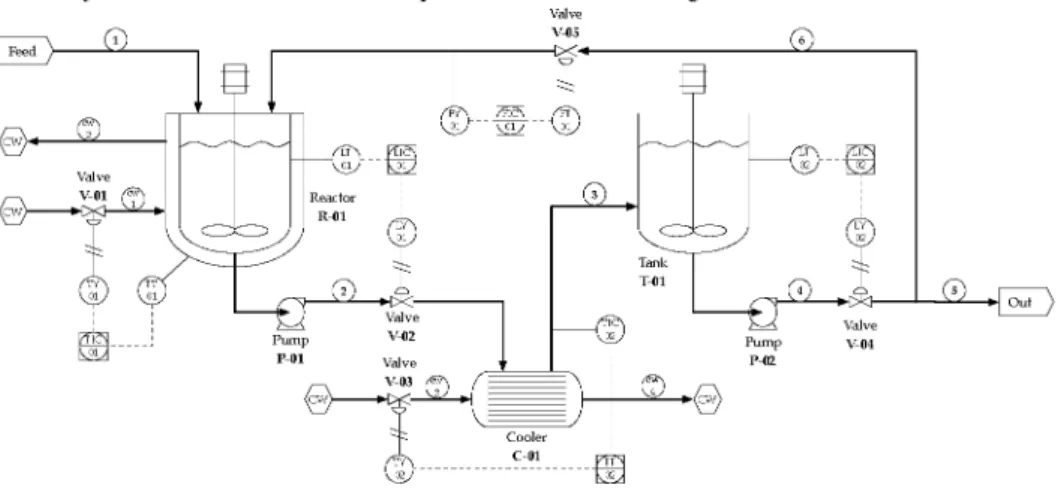
3.1. Process description

The process consists of a jacketed reactor, a cooler and a storage tank. An exothermic

reaction of isomerization in liquid phase is carried out in the reactor. Cooling water is

poured through the jacket to keep reactor temperature. The cooler is a shell and tube

heat exchanger with one shell pass and two tubes passes. There are also flve control

loops controlling the reactor level and temperature, cooler outlet temperature, tank level

and recycle flow. The P&ID of the process is shown in Fig. 1.

Fig. 1: Process P&I diagram.

3.2. Model description

The reactor and the tank are modeled using mass and energy balances. In both cases

perfect mixing is considered. The cooler has been modeled using a discretization of its

internal flow dynamics. The flve control loops are considered as Pls and they are tuned

using the Ziegler-Nichols method. The overall mathematical system consists of 41

EDOs, 54 constitutive equations and 10 flow constraints. There are 43 variables of

interest in the process concerning flows, molar fractions and temperatures.

3.3. Fault analysis

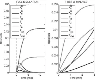
3.3.1. Fouling in the reactor jacket

This is a particularly common and severe problem because the heat transfer decreases

and the reaction can run away. The time evolution of the residuals is depicted in Fig. 2.

Notice that only the most relevant residuals are shown in the figure.

• Higher máximum: Cooling water flow.

• Lower máximum time: B molar fraction in the reactor.

• Higher initial slope: Jacket temperature.

• Higher steady-state valué: Cooling water flow.

Note that in the steady state variables such as reactor temperature and molar fractions in

the reactor go back to zero residual. This is because the control system keeps the reactor

variables under control. However, the flow to the jacket and the jacket temperature have

a non-zero residual in steady state. This information is consistent with the fault

described.

Tj

hR

JjR

rB

TR

Tj

hR

FULL SIMULATION FIRST 3 MINUTES

A molar fraction in the reactor

B molar fraction in the reactor

Reactor temperature

Jacket temperature

Reactor level

Reactor outlet flow

Cooling water flow to the jacket

0 5 10 Time (mln

Fig. 2: Fouling in the reactor jacket residuals.

A molar fraction in the reactor

B molar fraction in the reactor

Reactor temperature

Jacket temperature

Reactor level

Reactor outlet flow

Cooling water flow to the jacket

FULL SIMULATION FIRST 3 MINUTES

0 1 2 3

Time (mln)

Fig. 3. Residuals of a fault in the reactor level sensor.

3.3.2. Fault in the reactor level sensor

The faulty sensor provides a level lower than the real. The time evolution of the

residuals is shown in Fig. 3 and its parameters are:

• Lower máximum time: Reactor outlet flow. • Higher initial slope: Reactor outlet flow. • Higher steady-state valué: Cooling water flow.

The residuals shown in Fig. 3 are consistent with the fault described. At first the outlet flow varies a lot to compénsate the difference from the level set point (control system action) and then, the cooling water flow also increases to compénsate the increment of volume in the reactor.

3.3.3. On-line detection

Comparing figures 2 and 3 is obvious that the residuals of both faults are different and the parameters used to characterize them also differ. So if during normal operation of the plant we detect the pattern of any of these faults, we can identify them and corrective actions can be performed.

4. C o n c l u s i o n s a n d further w o r k

In this paper a new methodology for fault detection has been presented. This methodology is based on characterizing the fault type associating it to a set (pattern) of variables. This pattern has the variables and their time evolution. It is a self-learning approach as it can be programmed to genérate every potential fault in the system and compute the (automatically) residuals and, following the given criteria, establish the corresponding pattern to that fault. When used online it allows an early fault detection and besides it continúes with the learning process which is run in the background. This will genérate new patterns as well as will update existing (non working properly) ones. The methodology has been applied to an industrial case. The ongoing work is to apply the methodology to an industrial process and intégrate it with a sensor validation procedure that will permit to discrimínate bad plant data from trae faults. The methodology will also be integrated with the functional methodology developed D-higraphs that provides an easy way to follow how the status of the overall plant is changing and what the consequences of the fault will be (if not fixed on time).

Referen ees

A. Kulkarni, V.K. Jayaraman, B.D. Kulkarni (2005). Knowledge incorporated support vector machines to detect faults in Tennessee Eastman Process. Computers and Chemical Engineering, 29,2128-2133.

X. Bin He, W. Wang, Y. Pu Yang, Y. Hong Yang (2009). Variable-weighted Fisher discriminant analysis for process fault diagnosis. Journal of Process Control.

5. Yoon, J.F. MacGregor (2001). Fault diagnosis with multivariate statistical models part I: using steady state fault signatures. Journal of process control, 11, 387- 400.

L. Rokach (2007). Genetic algorithm-based feature set partitioning for classification problems. N. Vora, Tambe S.S., Kulkarni B.D. (1997). Counterpropagation neural Networks for fault detection and diagnosis. Computers and Chemical Engineering, 21, 2, 177-185.

M. Yong, X. Zheng, Y. Zheng, S. Youxian, W. Zheng (2007). Fault diagnosis based on Fuzzy Support Vector Machine with parameter tuning and Feature Selection. Chínese Journal of Chemical Engineering, 15, 2, 233-239.

A. Sundarraman, R. Srinivasan (2003). Monitoring transitions in chemical plants using enhanced trend analysis. Computers and chemical engineering, 27, 1455-1472.