Time Series Clustering using the Total Variation Distance
with Applications in Oceanography
Pedro C. Alvarez-Estebana∗ C. Eu´anb J. Ortegab
a Dept. de Estad´ıstica e Investigaci´on Operativa, Universidad de Valladolid.
Paseo de Bel´en, 7. 47005 Valladolid. Spain.
b CIMAT, A.C. Jalisco, s/n, Mineral de Valenciana. Guanajuato 36240, Mexico.
January 22, 2015
Abstract
A time series clustering algorithm based on the use of the total variation distance between normalized spectra as a measure of dissimilarity is proposed in this work. The oscillatory behavior of the series is thus considered the central characteristic for classification purposes. The proposed algorithm is compared to several other methods which are also based on features extracted from the original series and the results show that its performance is comparable to the best methods available and in some tests it outperforms the rest. As an application the algorithm is used to determine stationary periods for random sea waves, both in simulations and on a real data set, a problem in which changes between stationary sea states are usually slow.
Keywords: Total Variation Distance, Times Series Clustering, Spectral Analysis, Random Sea Waves, Hierarchical Clustering, Stationary Periods.
MSC classes: 62H30, 62M10, 62M15.
1
Introduction
In this work a clustering procedure for time series based on the use of the total variation distance between normalized spectral densities is proposed. The approach is thus based on classifying time series in the frequency domain by consideration of the similarity between their oscillatory characteristics.
In general, clustering is a procedure whereby a set of unlabeled data is divided into groups so that members of the same group are similar, while members of different groups
∗
Corresponding author. E-mail: [email protected]. Phone: +34 983 423930
differ as much as possible. The problem of clustering when the data points are time series has received a lot of attention in recent times. Liao [20] gives a revision of the field up to 2005 while Kavitha and Punithavalli [16] survey work on clustering of time series data streams, a problem we will not deal with in this paper. A thorough revision of the literature in recent years is outside the scope of this work, but the subject has found applications in very diverse fields such as the identification of similar physicochemical properties of amino acid sequences [31], analysis of fMRI data [12], detection of groups of stocks sharing synchronous time evolutions with a view towards portfolio optimization [4], finding groups of similar river flow time series for regional classification [8] and microarray data analysis [7], to name but a few.
According to Liao [20] there are three approaches to time series clustering: methods based on comparison of raw data, feature-based methods, where the similarity between time series is gauged through features extracted from the raw data, and methods based on parameters from models adjusted to the data. Our approach falls in the second category, and the feature used is the spectral density of the corresponding time series. The simi-larity between two time series is measured by the total variation distance between their normalized spectra. The total variation (TV) distance is frequently used to measure differ-ences between probability measures, and therefore requires the normalization of spectral densities, so that the integral of the normalized spectral density is equal to one. This is equivalent to normalizing the time series so that its variance is equal to one. Hence we focus on differences in the distribution of the variance as a function of frequency rather than differences in the total variance present. The use of the total variation distance for the analysis of spectral differences in the context of spectral analysis of random waves was
proposed by Alvarez-Esteban & Ortega [2] and also considered in Eu´an, et al. [9, 10].
Once the spectra for the time series have been estimated and normalized, the TV distances between all pairs are calculated and used to build a dissimilarity matrix, which is then fed to a hierarchical clustering algorithm. Several linkage criteria were used with an agglomerative algorithm and Dunn’s index was employed for deciding the optimal number of clusters.
Many clustering algorithms have been devised for time series, and to compare their
performance P´ertega and Vilar [29] proposed a series of tests. To test the efficiency of our
algorithm the same tests were used. Since our interest lies in applications to random wave data, another test using families of spectral densities frequently used in Oceanography was also carried out. These tests show that, in most cases, the performance of the proposed algorithm compares with the best available, and in some cases it outperforms the rest.
analysis is related with several features of interest, such as the significant wave height (Hs)
or the dominant or peak period (Tp), that can be computed from the spectral distribution or
from its moments (see, e.g, Ochi [26]). On the other hand, Gaussian models, beyond being a good first order approximation, allow obtaining explicit expressions for the distribution of parameters of interest for engineers and oceanographers.
However, both hypotheses, stationarity and Gaussianity, have limitations. It is clear that in the medium/long-term the sea is non-stationary. Thus, the use of stationary models is limited in time, depending on the specific sea conditions at the place of study. In other words, the sea state at a specific point can be regarded (or modeled) as an alternating sequence of stationary and transition periods (between the stationary periods).
The problem of duration of sea states is linked to the detection of change-points in time series. However, the methods employed to this effect usually assume that changes in the time series occur instantaneously or in a very brief period of time, which is not usually the case for waves, where changes take time to develop. This problem has been studied
by several authors from different points of view. Ortega and Hern´andez [28] compared
the results of using two methods, detection of changes by penalized contrasts proposed by Lavielle [17, 18, 19] and the smoothed localized complex exponentials (SLEX), introduced by Ombao et al. [27], with unsatisfactory results. Soukissian and Samalekos [34] propose a segmentation method for significant wave height based on determining periods of stability,
increase and decrease using time-series and local regression techniques. Hern´andez and
Ortega [14] consider a method based on calculating mean values over moving windows, and using a fixed-width band to determine change points in the wave-height data. Other studies (Soukissian and Theochari [35], Monbet and Prevosto [25], Monbet, Aillot and Prevosto [24]) have focused on the joint distribution of certain wave parameters, both from the point of view of estimation and from the point of view of simulation, with the purpose of obtaining duration distribution parameters through Monte Carlo methods. Jenkins [15] considers the problem from the perspective of estimating the fractal (Hausdorff) dimension. As an application of time series clustering we propose a new method for determining stationary periods for random waves, that takes into account the fact that transitions are not instantaneous and take some time to develop. The point of view switches from the detection of change points to the identification of time intervals during which the behavior of the wave height time series is stable. These time series are divided into 30-minute periods, a time interval which is usually considered to be long enough for a good estimation of the spectral density and short enough for stationarity to be a reasonable assumption. The clustering algorithm is then applied to the set of 30-minute intervals. If the clusters obtained are contiguous in time they are considered to be stationary intervals. The procedure also allows for the determination of transition intervals between successive stationary periods.
distance. Section 4 reports results from a simulation study based partly on P´ertega and Vilar [29] to compare the clustering algorithm with other methods previously proposed in the literature. In Section 5 two types of applications are considered, first, using simulated data that includes transition periods the performance of the algorithm is assessed, and second, an application to real wave data is discussed in detail. The paper closes with conclusions about the experiments performed.
2
Total Variation Distance
The total variation (TV) distance is one of the most widely used metrics between prob-ability measures. Although it can be defined in general probprob-ability spaces, we will focus
on the real line, R. Given P and Q, two probability measures in R, the total variation
distance between them is defined as:
dT V(P, Q) = sup{|P(A)−Q(A)|:A∈ B} (1)
whereB is the class of the Borel sets on the real line.
One important property of the TV distance is that it is bounded between 0 and 1, being 1 the largest possible distance between two given probabilities. This property can be easily deduced from the definition. Obviously it is positive, and taking into account
that for every Borel set A, 0 ≤ P(A), Q(A) ≤ 1 then, 0 ≤ |P(A)−Q(A)| ≤ 1 and the
inequalities remain valid if we take the supremum over the sets inB. A value of 1 for the
distance can be attained if, for example,P and Qhave disjoint supports.
This property is very useful in order to interpret distance values between two probabil-ities: values close to 1 mean that the two probabilities are quite different, while distance values close to 0 mean that these probabilities are very similar, almost equal. A statistical test to contrast the null hypothesis that the TV distance between two probabilities is less or equal to a given threshold has been recently developed in [3].
IfP and Qhave density functions (typically with respect to the Lebesgue measure µ),
f and g, the TV distance between them can be computed (see, e.g., Massart [23]) using
the following expression:
dT V(P, Q) = 1−
Z ∞
−∞
min(f, g)dµ (2)
This equation helps to graphically interpret the TV distance. If two densities f and g,
have TV distance equal to 1−α this means that they share a common area of size α.
Density f Density g Density f Density g
Density f Density g Density f Density g
Figure 1: The TV distance measures the similarity between the two densities. The blue (pink) area is the
value of the TV distance.
3
Spectral Clustering
As was mentioned in the introduction, our approach to stationary time series clustering is based on the use of the spectral distribution as a feature that sums up the oscillatory behavior of the series around its mean value. In a physical context, e.g. when considering series of measurements of sea surface height at a fixed point, the spectrum of the time series is interpreted as the distribution of the energy as a function of frequency. The integral of the spectral density is (proportional to) the total energy present, and is, of course, the variance of the series. Thus a normalization of the spectral density corresponds to a consideration of the frequency distribution of the energy, disregarding the total energy present. Spectral densities that are similar after normalization correspond to times series that have similar oscillatory behavior around their mean values, but may differ in variance.
Our approach considers the normalized spectra of the time series as the feature of interest for clustering, and the total variation distance between their spectra is used to measure the similarity between two time series. The proposed procedure is as follows:
• For each time series the spectral density is estimated. In our case we used the inverse
Fourier transform of the ACF, smoothed using a Parzen window with a bandwidth of length 100. This was done using the software WAFO [5], which runs on Matlab.
• The total variation distances between the normalized spectral densities are calculated
and used to build a dissimilarity matrix.
• This dissimilarity matrix is fed to an agglomerative hierarchical clustering algorithm.
We considered three different linkage criteria: complete, average and Ward. We used
the functionagnes in R[30].
• To choose the number of cluster when no external indication was available, Dunn’s
index is used. See section 5.2 for details.
4
Simulations
P´ertega and Vilar [29] proposed two simulation tests to compare the performance of several
clustering algorithms. These tests were reproduced to compare the performance of the algorithm proposed in this article, with the best algorithms available. We also carried out simulations to assess the performance of our method in the presence of slow changes.
Comparative study.
In their study, P´ertega and Vilar consider several dissimilarity criteria. For our purpose
we only considered those that were not model-based and had the best results in their tests plus the distance based on the cepstral coefficients, which was not included in their tests. In the time domain:
• The distance between the estimated autocorrelation functions with uniform weights:
dACF U(X, Y) =
X
i
( ˆρi,X−ρˆi,Y)2
1/2
• The distance between the estimated autocorrelation functions with decaying
geomet-ric weights:
dACF G(X, Y) =
X
i
p(1−p)i( ˆρi,X −ρˆi,Y)2
1/2
Let
IX(λk) =T−1
T
X
t=1
Xte−iλkt
2
be the periodogram for the time series X, at frequencies λk = 2πk/T, k = 1, . . . , n with
n = [(T −1)/2], with a similar definition for the other time series Y. The dissimilarity
criteria they considered in the frequency domain were:
• The Euclidean distance between the estimated periodogram ordinates:
dP(X, Y) =
1
n X
k
(IX(λk)−IY(λk))2
1/2
• The Euclidean distance between the normalized estimated periodogram ordinates:
dN P(X, Y) =
1
n X
k
(N IX(λk)−N IY(λk))2
1/2
whereN IX(λk) =IX(λk)/ˆγ0X, N IY(λk) =IY(λk)/ˆγ0Y, with ˆγ0X, ˆγ0Y the sample
vari-ances of the time seriesX andY, respectively.
• The Euclidean distance between the logarithm of the estimated periodogram
dLP(X, Y) =
1
n X
k
( logIX(λk)−logIY(λk))2
1/2
• The Euclidean distance between the logarithm of the normalized estimated
peri-odogram
dLN P(X, Y) =
1
n X
k
( logN IX(λk)−logN IY(λk))2
1/2
• The square of the Euclidean distance between the cepstral coefficients (the Fourier
coefficients of the expansion of the logarithm of the estimated periodogram)
dCEP(X, Y) = p
X
k
(θXk −θkY)2
where,θ0 =
R1
0 logI(λ)dλandθk=
R1
0 logI(λ) cos(2πkλ)dλ.
These dissimilarity measures were compared with the TV distance and theL1 distance
of the log spectra. As was mentioned before, three experiments were carried out, the first
two are those proposed by P´ertega and Vilar, and the third one used simulated data with
slow transitions.
1. Generate a group of time series of lengthT that have some special characteristic, in order to have well-defined groups.
2. Calculate the dissimilarity matrix for each of the different measures. Here we fix some of the parameters as follows:
• For the ACFG and ACFU distances the maximum lag is 25 and for the geometric
weights we takep= 0.05
• For the CEP measure we takep= 128.
• The spectra are estimated using the inverse Fourier transform of the smoothed
ACF function. For the smoothing we use a Parzen window with a bandwidth of length 100.
• A dissimilarity measure based on theL1 distance between the logarithms of the
spectral densities was added, which is defined as
dL1(f1, f2) =
1 2
Z
|log(f1(ω))−log(f2(ω))|dω.
3. The dissimilarity matrix is then used in a hierarchical clustering algorithm with the complete link.
4. The final groups are formed from the dendrogram by fixing the number kof groups.
5. In order to evaluate the rate of success in the m-th iteration, the following index
was used. Let {G1, . . . , Gg} and {C1, . . . , Ck}, be the set of the g real groups and a
k-cluster solution, respectively. Then,
Sim(C, G) = 1
g
g
X
i=1
max
1≤j≤kSim(Cj, Gi),
where
Sim(Cj, Gi) =
2|Cj∪Gi|
|Cj|+|Gi|
This must be calculated for each trial and the average is finally taken.
Experiment 1. In this experiment a series of ARIMA models are considered. In
each iteration we simulate one realization of sizeT, from each of the following 12 ARIMA
models proposed by Caiado et al. [6], six of which are stationary and six non-stationary.
a) AR(1) φ1 = 0.9 g) ARIMA(1,1,0) φ1 =−0.1
b) AR(2) φ1 = 0.95, φ2 =−0.1 h) ARIMA(0,1,0)
c) ARMA(1,1) φ1 = 0.95, θ1 = 0.1 i) ARIMA(0,1,1) θ1 = 0.1
d) ARMA(1,1) φ1 =−0.1, θ1=−0.95 j) ARIMA(0,1,1) θ1 =−0.1
e) MA(1) θ1 =−0.9 k) ARIMA(1,1,1) φ1 = 0.1, θ1=−0.1
0.0 0.1 0.2 0.3 0.4 0.5 0.6
0
2
4
6
8
Frequency (Hz)
AR(1)[.9] AR(2)[.95,−.1] MA(1)[−.9] MA(2)[−.95,−.1] ARMA(1,1)[.95,.1] ARMA(1.1)[−.1,−.95]
0.0 0.1 0.2 0.3 0.4 0.5 0.6
0
1
2
3
4
5
6
Frequency (Hz)
AR(1)[.5] AR(2)[.6,.2] MA(1)[.7] MA(2)[.8,−.6] ARMA(1,1)[.8,.2]
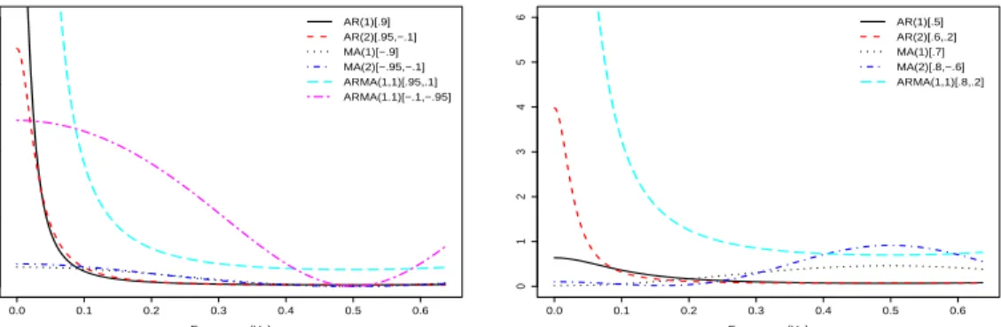
Figure 2: Spectra involved in experiment 1, stationary group (left) and in experiment 2 (right).
T= 200
N ACFG ACFU P NP LP LNP CEP TV L1
300 0.859 0.873 0.667 0.863 0.750 0.751 0.750 0.750 0.756
500 0.859 0.876 0.671 0.866 0.750 0.750 0.750 0.751 0.756
1000 0.861 0.878 0.674 0.870 0.750 0.750 0.750 0.751 0.756
Table 1: Results from Experiment 1. T is the length of the series,N is the number of replications. The
best result for each value ofN is underlined.
We expect that the clustering will divide the 12 series into two groups: stationary and non-stationary. Figure 2 (left) presents the spectral densities for the stationary processes. The figure shows that the spectra for the stationary series are not similar and so for the spectral methods we do not expect to get good results. Table 1 shows the rate of success, the ACFU gets the best results but when the spectra are not similar the TV distance works equally well.
Experiment 2. In this case 5 different ARMA models were considered, but with a different objective. For each model four series are generated, and the clustering algorithm is then applied to the 20 samples, to see if they are able to recover the original groups. The number of groups in the clustering algorithm is set to 4 and 5. The five ARMA models have the following parameters:
a) AR(1) φ1= 0.5 d) MA(2) θ1= 0.8, θ2 =−0.6
b) MA(1) θ1= 0.7 e) ARMA(1,1) φ1= 0.8, θ1= 0.2
c) AR(2) φ1= 0.6, φ2= 0.2
Figure 2 (right) shows the spectral densities for the five ARMA models. As can be seen, the spectra for the MA models are very similar so it may be difficult to distinguish them.
T = 200
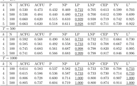
k N ACFG ACFU P NP LP LNP CEP TV L1
4 100 0.530 0.473 0.432 0.469 0.722 0.705 0.613 0.599 0.703
4 500 0.536 0.484 0.440 0.480 0.718 0.700 0.612 0.599 0.699
5 100 0.660 0.620 0.515 0.610 0.939 0.938 0.719 0.742 0.925
5 500 0.663 0.620 0.518 0.611 0.928 0.927 0.711 0.739 0.922
T = 500
k N ACFG ACFU P NP LP LNP CEP TV L1
4 100 0.592 0.568 0.490 0.561 0.733 0.732 0.711 0.664 0.730
4 500 0.585 0.561 0.492 0.558 0.733 0.732 0.708 0.667 0.731
5 100 0.745 0.683 0.561 0.687 0.998 0.798 0.820 0.852 0.995
5 500 0.741 0.685 0.566 0.683 0.999 0.798 0.817 0.846 0.996
T = 1000
k N ACFG ACFU P NP LP LNP CEP TV L1
4 100 0.614 0.583 0.537 0.582 0.733 0.733 0.730 0.708 0.733
4 500 0.615 0.586 0.536 0.587 0.733 0.733 0.730 0.714 0.733
5 100 0.806 0.728 0.600 0.714 1.000 0.800 0.873 0.907 1.000
5 500 0.805 0.737 0.604 0.719 1.000 0.800 0.874 0.914 1.000
Table 2: Results for Experiment 2. T is the length of the series, k the number of clusters and N the
number of replications. The best result for each value ofT is underlined.
2.
The LP distance works better for small or moderate-length series, however as T
in-creases the difference with the L1 distance diminishes, and for T = 1000 the results are
equally good. If we only compare the spectral distances that do not use the logarithm, the TV distance is better, with a success rate that is between 10% and 20% higher than the rest, including the ACF distances.
The methods that involved the logarithm of the spectra did not perform well when the original spectral were very close and the shape was similar. In order to explore this in more detail, we performed a third simulation experiment, based on parametric spectra that are frequently used in Oceanography.
Experiment 3. The last experiment is based on two different JONSWAP (Joint North-Sea Wave Project) spectra. This is a parametric family of spectral densities which is frequently used in Oceanography, and is given by the formula
S(w) = g
2
w5exp(−5w 4
p/4w4)γexp(
−(w−wp)2/2wp2s2)
whereg is the acceleration of gravity, s= 0.07 if w <=wp and s= 0.09 otherwise; wp =
π/Tp and γ = exp(3.484(1−0.1975(0.036−0.0056Tp/
√
Hs)Tp4/(Hs2))). The parameters
for the model are the significant wave heightHs, which is defined as 4 times the standard
0 0.1 0.2 0.3 0.4 0.5 0.6 0.7 0.8 0.9 0
0.5 1 1.5 2 2.5
Frequency (Hz)
Tp= 3.6 Tp= 4.1
0 0.1 0.2 0.3 0.4 0.5 0.6 0.7 0
0.05 0.1
Frequency (Hz)
Jonswap Tp=3.6
Jonswap Tp=4.2
Torsethaugen T
p=5
Figure 3: The JONSWAP spectra involved in experiment 3 (left) and the spectra involved in the
simula-tions based on transisimula-tions (right).
to the modal frequency of the spectrum. This spectral family was empirically developed after analysis of data collected during the Joint North Sea Wave Observation Project
(JONSWAP) [13]. It is a reasonable model for wind generated sea when 3.6√Hs ≤ Tp ≤
5√Hs.
The spectra considered both have significant wave height Hs equal to 3, the first has a
peak periodTp of 3.6
√
Hs while for the second Tp = 4.1
√
Hs.
Figure 3 (left) exhibits the JONSWAP spectra, showing that the curves are close to each other. As was mentioned in the comments on Experiment 2, this had the purpose of testing the performance of methods involving logarithms (LP and LNP), which had the best results in that experiment, under a different scenario. For data coming from similar spectra, sampling variability in the estimation of the spectral densities may be enhanced by the logarithm and this may have the effect of making more difficult the correct identification of the two groups.
Four series from each spectrum were simulated with the purpose of testing whether the different criteria were able to recover the original groups. Table 3 gives the results. In this case the method proposed in this work performs better than the rest, followed closely by ACFG. In this experiment, in general methods not using logarithms perform better than
those that use it. ForT = 1000 several methods are equally accurate.
5
Applications.
T = 100
k N ACFG ACFU P NP LP LNP CEP TV L1
2 100 0.783 0.769 0.623 0.764 0.669 0.662 0.654 0.786 0.641
2 500 0.785 0.771 0.624 0.762 0.671 0.655 0.669 0.790 0.657
T = 200
k N ACFG ACFU P NP LP LNP CEP TV L1
2 100 0.879 0.873 0.704 0.874 0.681 0.708 0.677 0.900 0.702
2 500 0.894 0.875 0.709 0.863 0.706 0.710 0.692 0.905 0.722
T = 1000
k N ACFG ACFU P NP LP LNP CEP TV L1
2 100 0.999 0.999 0.972 0.999 0.818 0.813 0.789 1.000 0.944
2 500 0.999 0.999 0.974 0.999 0.855 0.858 0.809 1.000 0.943
Table 3: Results from the Experiment 3. The best result for each value ofT is underlined.
function of frequency for the given sea state.
Typically, stationary sea states last for some time (hours or days), and then, due to changing weather conditions, sea currents, the presence of swell or other reasons, change to a different state. These changes do not occur instantaneously, but rather require a certain time to develop, during which there is a transition between the initial and final states. In this context, the usual segmentation methods that seek to determine change-points in a non-stationary time series do not work well, and a different point of view for the problem may be helpful: instead of looking for change-points, the idea is to identify short stationary intervals which have similar behavior, in terms of their spectral densities. If these intervals are contiguous in time, then it is reasonable to assume that they constitute a single (longer) stationary interval. The similarity is determined using the TV distance over normalized spectra, and the clustering procedure described in section 3.
5.1 Simulated Data
Further simulation studies were carried out to assess the performance of the clustering algorithm in the presence of transition periods. The main objective was to gauge the per-formance when slow transitions between stationary periods are present in a set of data. The simulations were carried out using the JONSWAP and Torsethaugen families of spectra. The Torsethaugen is a family of bimodal spectra used in Oceanography, which accounts for the presence of swell and wind-generated waves, and was also developed to model spectra observed in North-Sea locations. Details can be found in [36, 37].
In all cases the significant wave height (Hs) was set to 1; the simulated series starts
with waves from a stationary period of 4 hours (JONSWAP spectrum with peak period
Tp = 3.6), then a transition lasting 3 hours to another stationary period (JONSWAP
a third stationary period (Torsethaugen spectrum withTp = 5.0). Figure 3 (right) shows
the parametric spectra involved in the experiment. One thousand replications of this
scheme were simulated. The description of the method for simulating transition periods
can be seen in Eu´an, et al. [9].
The simulated data was divided into 30-minute intervals and the corresponding spectra
were estimated. Using these spectral densities, the clustering algorithm based on the
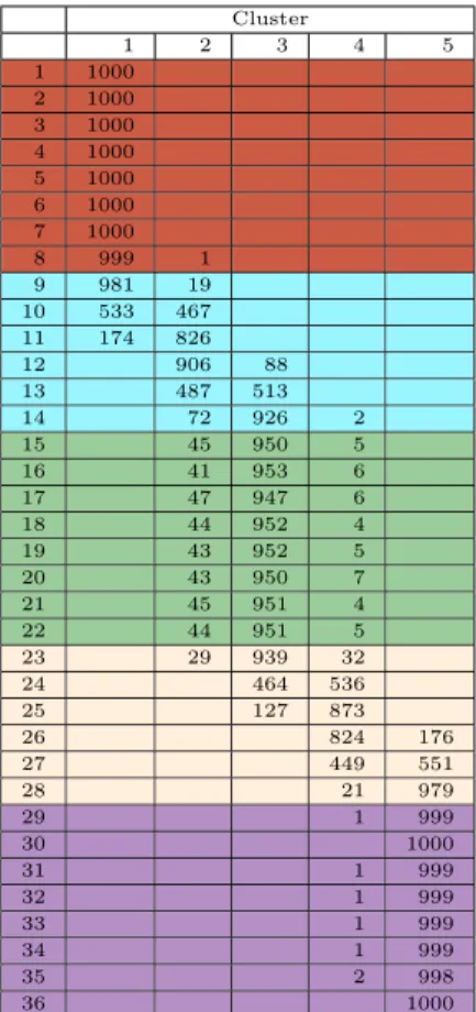
TV distance previously described was applied with three different link functions, complete, average and Ward. The algorithm was expected to recover five groups, the three stationary periods and two transitions. Tables 4 and 5 show the results for the 1000 replications. The row color stands for the original groups, for example intervals 1 to 8, colored in orange, represent the first group. The column corresponds to the group assigned by the clustering algorithm.
Cluster
1 2 3 4 5
1 1000 2 1000 3 1000 4 1000 5 1000 6 1000 7 1000
8 999 1
9 981 19
10 533 467
11 174 826
12 906 88
13 487 513
14 72 926 2
15 45 950 5
16 41 953 6
17 47 947 6
18 44 952 4
19 43 952 5
20 43 950 7
21 45 951 4
22 44 951 5
23 29 939 32
24 464 536
25 127 873
26 824 176
27 449 551
28 21 979
29 1 999
30 1000
31 1 999
32 1 999
33 1 999
34 1 999
35 2 998
36 1000
Table 4: Results for the simulated transition
data using the Complete linkage function and 5 groups
Cluster
1 2 3
1 1000 2 1000 3 1000 4 1000 5 1000 6 1000 7 1000 8 1000 9 1000
10 980 20
11 815 185
12 565 435
13 188 812
14 5 995
15 1 999
16 1000 17 1000 18 1000 19 1000 20 1000 21 1000 22 1000 23 1000
24 863 137
25 585 415
26 297 703
27 57 943
28 1000 29 1000 30 1000 31 1000 32 1000 33 1000 34 1000 35 1000 36 1000
Table 5: Results for the simulated transition
data using the Complete linkage function and 3 groups
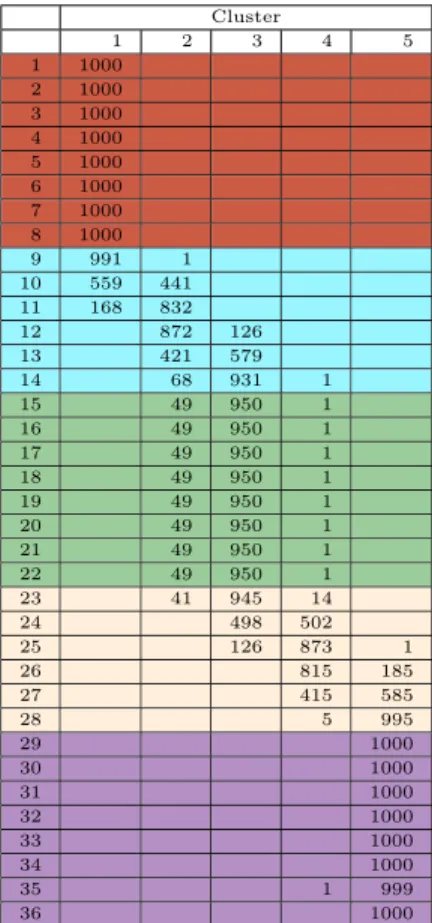
the right result. For the central stationary period the success rate is around 95%. The algorithm has a harder time identifying the transition periods, which is reasonable since these are not homogeneous groups. In particular, intervals at the beginning and at the end of a transition period are classified as belonging to the nearby stationary period over 90% of the time in all cases. This is also reasonable since the transition is slow and due to the sampling variability in the estimation of the spectral densities, such small differences are difficult to detect. Tables 6 and 7 show the results for the average and Ward link functions respectively. The results are similar in all cases. The Ward link gives better results for the central stationary period while the complete and average links gives better results in the initial and final stationary periods.
Cluster
1 2 3 4 5
1 1000 2 1000 3 1000 4 1000 5 1000 6 1000 7 1000 8 1000
9 991 1
10 559 441
11 168 832
12 872 126
13 421 579
14 68 931 1
15 49 950 1
16 49 950 1
17 49 950 1
18 49 950 1
19 49 950 1
20 49 950 1
21 49 950 1
22 49 950 1
23 41 945 14
24 498 502
25 126 873 1
26 815 185
27 415 585
28 5 995
29 1000 30 1000 31 1000 32 1000 33 1000 34 1000
35 1 999
36 1000
Table 6: Results for the simulated transition
data using the Average linkage function and 5 groups
Cluster
1 2 3 4 5
1 1000
2 998 2
3 998 2
4 996 4
5 997 3
6 994 6
7 997 3
8 996 4
9 963 37
10 443 557
11 96 904
12 2 905 93
13 500 500
14 72 928
15 20 979 1
16 20 978 2
17 22 977 1
18 22 976 2
19 23 976 1
20 19 978 3
21 19 980 1
22 20 978 2
23 11 953 36
24 376 624
25 56 944
26 890 110
27 533 467
28 31 969
29 1 999
30 1000
31 1000
32 1 999
33 2 998
34 1000
35 1 999
36 1 999
Table 7: Results for the simulated transition
data using the Ward linkage function and 5 groups
are correctly assigned within the same group. Transition intervals tend to be classified in the closest stationary group. These results could be used in a two-tier process, in which, in a given realization and using the results of the clustering algorithm, the intervals at the border would be tested to decide whether they really belong to the same group as the rest, or they should be considered as belonging to a transition period and moved outside the cluster. This idea will not be further developed in this work.
5.2 Real Data Analysis
Our starting point in this section is the idea that sea states at a fixed point on the sea surface can be modeled as a sequence of alternating stationary and transition periods. With this structure in mind and based on the results of the simulations shown in Section 5.1, we carried out a clustering analysis over a real data set in order to detect these periods. We used real wave data obtained from the U. S. Coastal Data Information Program (CDIP) website. The data come from buoy 106 (51201 for the National Data Buoy Center), located in Waimea Bay, Hawaii, at a water depth of 200 m. and correspond to 192 30-minute intervals in January 2003, a total of 96 hours (4 days).
Figure 4 shows both significant wave height (black) and spectral peak frequency (blue)
for this data set. This plot shows that Hs starts with values around 2 meters and then,
about the middle of the time interval, increases in a short time to values around 3.7-4 meters where it remains for the rest of the period. On the other hand, the spectral peak
frequency starts the period slightly increasing, then starts to decrease asHs increases, to
remain low for the rest of the period.
The clustering analysis was carried out in two different ways. Initially the complete data set, comprising the 192 time intervals, was considered. Alternatively the data set was divided in two groups of equal length, group 1 including intervals 1 - 86 and group 2 intervals 87 - 192. A comparison of the results obtained in each case gives indications about the consistency of the proposed method and also allows for the evaluation of possible boundary effects in the segmentation procedure.
As in Section 5.1, for each 30-minute interval the spectral density was computed and normalized, and the matrix of total variation distances between these spectra was calcu-lated. This matrix is the input for the agglomerative hierarchical clustering procedure. We tried the three main linkage functions: complete, average and Ward, with similar results.
Unlike the simulations of Section 5.1 where the number of clusters is known, here
this number is unknown. In order to decide the appropriate number of clusters, k, to be
considered in the analysis a suitable method should be chosen. A good review of available
methods to assess the value of k can be found, for example, in chapter 17 of Gan et al.
1
2
3
4
5
Buoy 106, January 2003
Time interval
Hs (m)
0 50 100 150
0.36
0.46
Frequency (Hz)
Hs (m) Peak frequency (Hz)
Figure 4: Significant wave height (black) and peak frequency (blue) for buoy 106 from Jan 1st to Jan 4th,
2003.
VD(k) = min
1≤i≤k
min
i+1≤j≤k
D(Ci, Cj)
max1≤h≤kdiam(Ch)
,
where k is the number of clusters, D(Ci, Cj) is the distance between clusters Ci and Cj,
and diam(Ch) is the diameter of clusterCh.
From the definition of VD it is clear that high values point to suitable values of k.
The computation of this index was carried out using theclv package in R [30]. Among the
available metrics to computeD(Ci, Cj) anddiam(Ch) the average was selected. The results
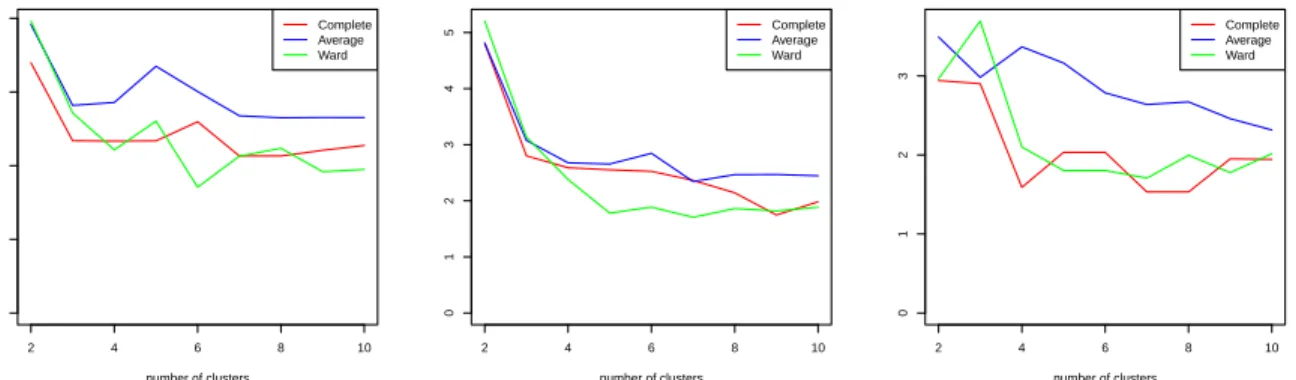
for the three clustering procedures and the three linkage functions are shown in Figure 5. The main conclusion is that there is a good degree of agreement between the three linkage functions for each clustering procedure. Plot (a) for the clustering over the whole 192-time intervals indicates the existence of 5 (average, Ward) or 6 (complete) groups. Dunn’s index in plot (b) for the first 86-time periods indicates clearly the existence of two groups, and finally, plot (c) for the second half of the period points to 2 (complete), 3 (Ward) or 4 (average) groups, depending on the linkage function.
Figures 6 and 7 show the result of the clustering procedure for the average and Ward
linkage function, respectively, and k chosen using Dunn’s index. The first interesting
point to note in both figures is that, broadly speaking, the clustering procedure captures the time structure in the data. In other words, using only information about the total variation distance between normalized spectral densities, the clustering procedure groups in the same cluster time intervals that are contiguous, and this is valid except for a few time intervals in each case.
Plot (a) of Figure 6 shows the groups for the whole time interval using k= 5 clusters
and the average linkage function. In this plot, the period of time between intervals 1 and
2 4 6 8 10
0
1
2
3
4
(a) Dunn's index, intervals 1−192
number of clusters
Complete Average Ward
2 4 6 8 10
0
1
2
3
4
5
(b) Dunn's index, intervals 1−86
number of clusters
Complete Average Ward
2 4 6 8 10
0
1
2
3
(c) Dunn's index, intervals 87−192
number of clusters
Complete Average Ward
Figure 5: Dunn’s index for the three clustering processes using complete, average and Ward linkage
functions: (a, left) intervals 1-192, (b, middle) intervals 1-86 and (c, right) intervals 87-192.
(red) comprises most of the initial 56 time intervals, with the exception of 4 of them, 22, 23, 25 and 34, which belong to the fourth cluster. It corresponds to a period of time during
which both Hs and Tp are stable. The second cluster (57-87, in blue) includes the rest of
the intervals in the first half, and represents an uninterrupted sequence of time intervals. This is very similar to the clustering obtained for time intervals 1 - 86, represented in plot (b). In this case there are only two groups, and the main difference with the first half of plot (a) is the starting point of the second cluster, which has moved to the left, to interval 53. The other difference is that now intervals 22, 23, 25 and 34 are assigned to the first cluster, which becomes a single block.
The third group (82-97, purple) in plot (a) corresponds to the initial stages of growth
for Hs, and is followed by a sequence of 6 intervals belonging to cluster 1. The fourth
cluster (104-179 except 153 and 157, green) is the largest and includes almost all intervals
of the period whereHs oscillates around 3.7-4 m. There are two red intervals that break
the time continuity of this cluster, 153 and 157, which belong to cluster 1. Finally, the fifth cluster (180-192, yellow) appears at the end of this last period, and is also an uninterrupted sequence of time intervals. Comparing with plot (c), which corresponds to intervals 87-192 divided into 4 groups, we see that the first interval (red) is classified as a cluster on its own. In plot (a) this interval is the last in cluster 2 (dark blue). The second cluster (green) in plot (c) coincides with cluster 3 in plot (a). The third cluster (purple) encompasses the fourth cluster (green) in plot (a) plus the segments included in cluster 1 (red) for this half of the data, as well as 8 intervals included in cluster 5 (yellow). Finally, cluster 4 (light blue) in plot (b) groups the rest of the intervals in cluster 5 (yellow) of plot (a).
0
1
2
3
4
5
(a) Intervals 1−192, k=5
Hs (m)
0 50 100 150
0
1
2
3
4
5
(b) Intervals 1−86, k=2
Hs (m)
0 50 100 150
0
1
2
3
4
5
(c) Intervals 87−192, k=4
Hs (m)
0 50 100 150
Figure 6: Clustering results using the average linkage functions.
in which temporary changes in the sea conditions (the presence of swell or local variations in the wind, for example) produce changes that disappear once these temporary conditions cease, as may be the case for intervals 21, 22, 24, 34, 153 and 157.
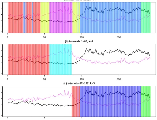
The three plots in Figure 7 correspond to the results with the Ward linkage function. Plot (a) shows the complete time interval with 5 groups, while plots (b) and (c) correspond to the two halves with 2 and 3 clusters, respectively, as suggested by the Dunn index. As can be seen the results for the second half are almost identical in both cases, since only the first interval (87) is classified differently in plot (a). As for the first half, results in both cases are very similar, with a second group (56-86) in plot (b) that corresponds exactly to cluster 4 in plot (a), while the first cluster in plot (b) gathers together the rest of the first half, with intervals coming from clusters 1, 2 and 3 in plot (a).
0
1
2
3
4
5
(a) Intervals 1−192, k=5
Hs (m)
0 50 100 150
0
1
2
3
4
5
(b) Intervals 1−86, k=2
Hs (m)
0 50 100 150
0
1
2
3
4
5
(c) Intervals 87−192, k=3
Hs (m)
0 50 100 150
Figure 7: Clustering results using the Ward linkage functions.
in the Ward case.
Summing up, this analysis suggests that there may be three stationary intervals in the data and three transition periods. The stationary intervals are segments 1 - 44, 56-87 and 104-179, with the rest of the intervals belonging to transition periods.
6
Conclusions
In this paper a new method for time series clustering was proposed. The method is based on using the total variation distance between normalized spectra as a measure of dissimilarity between time series. Simulation results (Sec. 4) show that the method has a performance that is comparable to the best clustering methods based on features extracted from the raw data, and in certain cases it performs better than the rest. Simulations (Sec. 5.1) also show that the method is capable of detecting stationary periods in situations where slow transitions between stationary states occur.
the average and Ward linkage functions, presented in Sec. 5.2, show a good agreement for the two linkage functions. The results also show that the results are consistent when the clustering method is applied over intervals of different length.
7
Acknowledgements
The software WAFO developed by the Wafo group at Lund University of Technology, Sweden, available at http://www.maths.lth.se/matstat/wafo was used for the calculation of all Fourier spectra and associated spectral characteristics. The data for station 106 were furnished by the Coastal Data Information Program (CDIP), Integrative Oceanographic Division, operated by the Scripps Institution of Oceanography, under the sponsorship of the U.S. Army Corps of Engineers and the California Department of Boating and Waterways (http://cdip.ucsd.edu/).
This work was partially supported by CONACYT, Mexico, Proyecto An´alisis
Es-tad´ıstico de Olas Marinas, Fase II. J. Ortega wishes to thank Prof. Adolfo J. Quiroz for several fruitful conversations of the topic of this paper. P.C. Alvarez Esteban wishes to acknowledge CIMAT, A.C., the Spanish Ministerio de Ciencia y Tecnolog´ıa, grants
MTM2011-28657-C02-01 and MTM2011-28657-C02-02 and the Consejer´ıa de Educaci´on
de la Junta de Castilla y Le´on, grant VA212U13 for their financial support.
References
[1] Christian Aage, Tom D. Allan, David J.T. Carter, Georg Lindgren, and Michel
Olagnon. Oceans from Space. Editions Ifremer, Brest, France, 1998.´
[2] P.C. Alvarez-Esteban and J. Ortega. Changes in wave spectra and total variation
distance. In Proceedings of the 22 nd International Offshore and Polar Engineering
Conference, volume 3, pages 660–665. ISOPE, 2012.
[3] Pedro C. Alvarez-Esteban, E. del Barrio, J. A. Cuesta-Albertos, and Carlos Matr´an.
Similarity of samples and trimming. Bernoulli, 18:412–426, 2012.
[4] Nicolas Basalto and Francesco De Carlo. Clustering financial time series. In Hideki
Takayasu, editor, Practical Fruits of Econophysics, pages 252–256. Springer Tokyo,
2006.
[5] P.A. Brodtkorb, P. Johannesson, G. Lindgren, I. Rychlik, E. Ryd´en, and E. Sj¨o.
WAFO - a Matlab toolbox for analysis of random waves and loads. In Proc. 10th
[6] J. Caiado, N. Crato, and D. Pe˜na. A periodogram-based metric for time series
classi-fication. Computational Statistics and Data Analysis, 50:2668 – 2684, 2006.
[7] C. Chira, J. Sedano, J.R. Villar, C. Prieto, and E. Corchado. Gene clustering in time
series microarray analysis. In A. Herrero, B. Baruque, F. Klett, A. Abraham, V. Sn´asel,
A.C.P.L.F. de Carvalho, P. Garc´ıa Bringas, I. Zelinka, H. Quinti´an, and E. Corchado,
editors, International Joint Conference SOCO’13-CISIS’13-ICEUTE’13, volume 239
of Advances in Intelligent Systems and Computing, pages 289–298. Springer Interna-tional Publishing, 2014.
[8] Marcella Corduas. Clustering streamflow time series for regional classification.Journal
of Hydrology, 407(1–4):73 – 80, 2011.
[9] C. Eu´an, J. Ortega, and P.C. Alvarez-Esteban. Detecting changes in wave spectra
using the total variation distance. In Proceedings of the 23 rd International Offshore
and Polar Engineering Conference, volume 3, pages 824–830. ISOPE, 2013.
[10] C. Eu´an, J. Ortega, and P.C. Alvarez-Esteban. Detecting stationary intervals for
random waves using time series clustering. In Proceedings of the 33 rd International
Conference on Ocean and Arctic Engineering, pages 1–7. ASME, 2014.
[11] Guojun Gan, Chaoqun Ma, and Jianhong Wu. Data clustering - Theory, Algorithms,
and Applications. SIAM, 2007.
[12] Cyril Goutte, Peter Toft, Egill Rostrup, Finn ˚A. Nielsen, and Lars Kai Hansen. On
clustering fmri time series. NeuroImage, 9(3):298 – 310, 1999.
[13] K. Hasselmann, T.P. Barnett, E. Bouws, H. Carlson, D.E. Cartwright, K. Enke, J.A. Ewing, H. Gienapp, D.E. Hasselmann, P. Kruseman, A. Meerburg, P. Mller, D.J. Olbers, K. Richter, W. Sell, and H. Walden. Measurements of wind-wave growth and swell decay during the joint north sea wave project (jonswap). Ergnzungsheft zur Deutschen Hydrographischen Zeitschrift Reihe, A 12, Deutsches Hydrographisches Institut Hamburg, 1973.
[14] Jos´e B. Hern´andez C. and J. Ortega. A comparison of segmentation procedures and
analysis of the evolution of spectral parameters. In Proceedings 17th. International
Offshore and Polar Engineering Conference, volume 3, pages 1836–1842. ISOPE, 2007.
[15] A.D. Jenkins. Wave duration/persistence statistics, recording interval, and fractal
di-mension. International Journal of Offshore and Polar Engineering, 12:109–113, 2002.
[16] V Kavitha and M Punithavalli. Clustering time series data stream-a literature survey.
[17] M. Lavielle. Optimal segmentation of random processes. IEEE Transaction on Signal Processing, 46:1365–1373, 1998.
[18] M. Lavielle. Detection of multiple changes in a sequence of dependent variables.
Stochastic Processes and their Applications, 83:79–102, 1999.
[19] M. Lavielle and C. Lude˜na. The multiple change-points problem for the spectral
distribution. Bernoulli, 65:845–869, 2000.
[20] T. Warren Liao. Clustering of time series data – a survey. Pattern Recognition,
38:1857–1874, 2005.
[21] M.S. Longuet-Higgins. The statistical analysis of a random moving surface. Philos.
Trans. Roy. Soc. London, Ser. A, 249(966):321–387, 1957.
[22] E.A. Maharaj and P. D’Urso. Fuzzy clustering of time series in the frequency domain.
Information Sciences, 181:1187 – 1211, 2011.
[23] Pascal Massart. Concentration Inequalities and Model Selection. Springer, Berlin,
2007.
[24] V. Monbet, P. Aillot, and M. Prevosto. Survey of stochastic models for wind and sea
state time series. Probabilistic Engineering Mechanics, 22:113–126, 2007.
[25] V. Monbet and M. Prevosto. Bivariate simulation of non stationary and non gaussian
observed processes. application to sea state parameters. Applied Ocean Res., 23:139–
145, 2001.
[26] Michael K. Ochi. Ocean Waves. The Stochastic Approach. Cambridge Ocean
Tech-nology Series. Cambridge Univ. Press, 1998.
[27] H. Ombao, J. Raz, R. Von Sachs, and W. Guo. The SLEX model of a non-stationary
random process. Ann. Inst. Statist. Math., 52(1):1–18, 2002.
[28] J. Ortega and Jos´e B. Hern´andez C. A comparison of two methods for spectral
analysis of waves. In Proceedings 16th. International Offshore and Polar Engineering
Conference, volume 3, pages 45–52. ISOPE, 2006.
[29] Sonia P´ertega D´ıaz and Jos´e A. Vilar. Comparing several parametric and
nonparamet-ric approaches to time series clustering: A simulation study. Journal of Classification,
27:333–362, 2010.
[30] R Core Team. R: A Language and Environment for Statistical Computing. R
[31] Alexios Savvides, Vasilis J Promponas, and Konstantinos Fokianos. Clustering of
biological time series by cepstral coefficients based distances. Pattern Recognition,
41(7):2398–2412, 2008.
[32] C.T. Shaw and G.P. King. Using cluster analysis to clasify time series. Physica D,
58:288–298, 1992.
[33] Robert H. Shumway. Time-frequency clustering and discriminant analysis. Probability
and Statistics Letters, 63:307–314, 2003.
[34] T.H. Soukissian and P.E. Samalekos. Analysis of the duration and intensity of sea
states using segmentation of significant wave height time series. In Proceedings 16th.
International Offshore and Polar Engineering Conference, volume 3, pages 45–52. ISOPE, 2006.
[35] T.H. Soukissian and Z. Theochari. Joint occurrence of sea states and associated
dura-tions. In Proceedings 11th. International Offshore and Polar Engineering Conference,
volume 3, pages 33–39. ISOPE, 2001.
[36] K. Torsethaugen. A two-peak wave spectrum model. InProceedings 18th. International
Conference on Ocean, Offshore and Artic Engineering (OMAE 1993), volume II, pages 175–180, 1993.