Study on the efficiency in the numerical integration of size-structured population models: Error and computational cost

Contents lists available atScienceDirect

Journal of Computational and Applied

Mathematics

journal homepage:www.elsevier.com/locate/cam

Study on the efficiency in the numerical integration of

size-structured population models: Error and computational

cost

Q1

∧

O.

∧

Angulo

a,∗

,

∧

J.C.

∧

López-Marcos

b

,

∧

M.A.

∧

López-Marcos

b

a_{Departamento de Matemática Aplicada, ETSIT, Universidad de Valladolid, Pso. Belén 5, 47011 Valladolid, Spain}

b_{Departamento de Matemática Aplicada, Facultad de Ciencias, Universidad de Valladolid, Pso. Belén 7, 47011 Valladolid, Spain}

a r t i c l e i n f o

Article history:

Received 15 October 2014

Received in revised form 23 February 2015

MSC:

92D25 92D40 65M25 65M12 35B40

Keywords:

Structured population models Numerical methods Efficiency

a b s t r a c t

We describe a procedure which is useful to select an appropriate numerical method in a size-structured population model. We consider four different numerical methods based on finite difference schemes or characteristics curves integration. We compute an analytical approximation in terms of the discretization parameters for the theoretical error principal terms and the computational cost. Thus, we show the efficiency curve that allows to select the best relationship between the discretization parameters for each numerical method. Finally, we obtain the most efficient numerical method for each test.

©2015 Published by Elsevier B.V.

1. Introduction

1

We will consider a well-known model describing the evolution of a population which is structured by meansofa physio-2

logical variable that usually is named as size. In particular we consider a model that consists of a nonlinear partial differential 3

equation with nonlocal terms (the population balance law) 4

ut

+

(

g

(

x

,

Ig

(

t

),

t

)

u

)

x

= −

µ(

x

,

Iµ

(

t

),

t

)

u

,

xmin

<

x

<

xmax

,

t

>

0

,

(1.1) 5

a nonlinear and nonlocal boundary condition that represents the birth law 6

g

(

xmin

,

Ig

(

t

),

t

)

u

(

xmin

,

t

)

=



xmax

xmin

α(

x

,

I_α

(

t

),

t

)

u

(

x

,

t

)

dx

,

t

>

0

,

(1.2)

7

and an initial condition 8

u

(

x

,

0

)

=

u0

(

x

),

xmin

≤

x

≤

xmax

,

(1.3)

9

∗_{Corresponding author. Tel.: +34 983 423000x5835; fax: +34 983 423661.}

E-mail addresses:oscar@mat.uva.es(O. Angulo),lopezmar@mac.uva.es(J.C. López-Marcos),malm@mac.uva.es(M.A. López-Marcos). http://dx.doi.org/10.1016/j.cam.2015.03.022

whereI_µ

(

t

),

I_α

(

t

)

andIg

(

t

)

are defined by 1

I_µ

(

t

)

=



xmax

xmin

γ

µ

(

x

)

u

(

x

,

t

)

dx

,

t

≥

0

,

(1.4) 2

I_α

(

t

)

=



xmax

xmin

γ

α

(

x

)

u

(

x

,

t

)

dx

,

t

≥

0

,

(1.5) 3

Ig

(

t

)

=



xmax

xmin

γ

g

(

x

)

u

(

x

,

t

)

dx

,

t

≥

0

.

(1.6) 4

The independent variablesxandtrepresent size and time, respectively. The valuesxminandxmaxrepresent the minimum 5 and maximum size, respectively. The dependent variableu

(

x

,

t

)

is the size-specific density of individuals with sizexat time 6 t. We assume that the size of any individual varies according to the next ordinary differential equation 7

dx

dt

=

g

(

x

,

Ig

(

t

),

t

).

(1.7) 8

The functionsg

, α

and

µ

represent the growth, the fertility and mortality rate, respectively. These are usually called the 9 vital functions and define the life history of an individual. Functionsg

, α

and

µ

are nonnegative. Note that all the vital func- 10 tions depend on the sizex(the structuring internal variable) and on the timet. The explicit time dependence can reflect the 11 influence of some environmental changes on the vital functions or a seasonal

∧

behaviorof the population. These functions 12 also depend on the total amount of individuals in the population by means of the weighted functionsIg

(

t

),

Iα

(

t

)

andIµ

(

t

)

, 13 which represent a way of weighting the size distribution density in order to model the diverse influence of the individuals 14

of different sizes on the life conditions. 15

We can find an extensive study on physiologically structured population models, with analytical studies of aspects such 16 as derivation, existence and uniqueness, smoothness and the asymptotic

∧

behaviorof solutions in [1–3]. In particular, this 17 size-structured population model has been studied for the last three decades and the properties of existence and uniqueness 18 of solutions was given in [4,5]. It has been successfully applied to the study of different real population problems. In order 19 not to be exhaustive we can mention its application to the cellular dynamics [6,7], the forest dynamics that employs a 20 hierarchical version [8,9],

∧

Daphniamagnapopulation studies [10], etc. 21 The increase in the biological realism in such a model is achieved at the expense of a loss in mathematical tractability. 22 Moreover, when such models include nonlinearities and environmental dependence on the different physiological rates, the 23 use of efficient methods that provide a numerical approach is the most suitable mathematical tool for studying the problem 24 and, indeed, it is often the only one available. Nevertheless, the numerical approach to these equations has important 25 drawbacks because they are usually nonlinear equations and the nonlinearities in the partial differential equation and the 26 nonlocal boundary condition are caused by nonlocal terms. A revision of the numerical schemes proposed for the solution 27 of this problem was made in [11]. Also, the numerical integration allows us the study of some other qualitative properties 28 as, for example, the long-time

∧

behaviorin real data problems, and they shown their effectiveness [6–8]. 29

The choice of a suitable numerical method for the integration of the problem is an important challenge. The convergence 30 is the main property we look for. In general, it means that the numerical solution is close to a representation of the exact 31 solution as the discretization parameters go to zero. The order of convergence quantifies the rate of convergence of this 32 approach with respect to the discretization parameters, and it is quite important too. Also it is necessary to evaluate the 33 computational cost which quantifies the effort needed to obtain the numerical approximation. One way to measure it is the 34 time spent to derive the numerical results. This time increases with the accuracy or the complexity of the numerical scheme. 35 In this work, we will pay attention to the relationship between the global error and the computational cost. First, we shall 36 try to obtain the most efficient relation to solve the problem between the discretization parameters for a given numerical 37 method. Next, we shall compare diverse numerical methods for a given problem to look for the most efficient. 38 The order of a numerical method depends strongly on the smoothness properties of the theoretical solution and, for 39 example, compatibility between initial and boundary conditions must be held and the data functions should be regular. We 40 believe that for real problems with empirical data, the conditions needed to obtain a convergence order greater than two are 41 too demanding. On the other hand, first convergence order method presents a lack of efficiency in comparison to the second 42 order ones. So, second order schemes maintain a good compromise between the required smoothness and the efficiency of 43

the schemes. 44

We will employ four second order numerical methods developed and analyzed in different works. Two of them are based 45 on a finite-difference discretization (Lax–Wendroff and Box schemes) [12] and the others are based on a characteristics 46 curves integration, the first one considers all the nodes in the spatial grid,

∧

aggregationgrid node method (AGN), and the 47

second one uses a selection procedure to keep constant the number of spatial grid nodes, selection grid nodes method 48

(SGN) [11]. We obtained their convergence order in [12,13]. 49

In the following section, we introduce the procedure and we apply it to several theoretical test problems. ∧

Inthe final 50 section, we present the procedure in a real data problem for which we do not know the exact solution. We describe briefly 51

2. Analytical approximation to efficiency

1

The numerical methods considered involve two discretization parameters: one step sizekused for the time integration, 2

and the other onehrelated to the size variable. In the theoretical analysis of the error of a second order method, it is typical 3

to obtain a bound of the global error in the form 4

Eh,k

=

C1h2

+

C2k2

,

(2.1)

5

withC1andC2positive constants. As the parameters go to zero, we consider this expression as the representative part of 6

the exact error and, for our purposes, we admit it as a valid approximation to the global error of a specific second order 7

numerical method. 8

On the other hand, it is natural to consider that computational cost depends on the size of the problem, which is given by 9

the size of the system of equations that can be represented in terms of the discretization parameters. In [14], it is declared 10

that the measure of the work in complex algorithms is not linear and follows a power law. However, taking into account that 11

we discretize two different variables in a different way, we do not use the same power for both discretization parameters 12

(as we will see, numerical experiments corroborate such assumption). Then, we establish 13

Ch,k

=

C3hakb

,

(2.2)

14

withaandbnegative real numbers, andC3positive. ConstantsC1

,

C2

,

C3

,

aandb, that appears in the error and cost expres-15

sions of the numerical method depend on the specific problem being approximated. 16

From numerical simulations of the method, it is usual to analyze its efficiency through log–log efficiency charts: the verti-17

cal axis correspond to the error and the horizontal axis is the cost. So, for different values of the discretization parameters, we 18

plot the error produced for the corresponding approximation versus the computational effort required. When we compare 19

two different methods in the efficiency plot, we prefer the method that gives more accuracy for the same computational 20

effort (or, in other words, the method that provides the cheapest way of obtaining a prescribed precision). 21

On the other hand, when we consider a specific numerical method for the approximation of a problem, we consider what 22

the best choice of the discretization parameters is. Here, we look for the best relationship betweenhandkfor each problem: 23

that is, we assume that 24

k

=

r h

,

(2.3)

25

withra fixed positive constant. So, our purpose is to select the most efficient value ofr. From expressions(2.1)and(2.2), 26

and assuming(2.3), we can write the error in terms of the cost: 27

Eh

=

(

C1

+

C2r2

)



Ch

C3rb



_a+2_b

.

(2.4)

28

In the log–log representation, we have 29

logEh

=

log

C1

+

C2r2

(

C3rb

)

2 a+b

+

2

a

+

blogCh

.

(2.5)

30

Note that, for eachrfixed, different values ofhprovide a line with the negative slope 2

/(

a

+

b

)

(the error decreases as the 31

cost increases), and this slope isrindependent (the lines associated to a specific method, and corresponding to different 32

values ofr, are parallel). So, the most efficient line corresponds to the value ofrwhich minimizes the first term on the right 33

hand size of(2.5). It is easy to see that such minimum is reached at 34

r

=



C1 C2 b

a

.

(2.6)

35

So, if we compare different methods for a problem, for each method we take the optimal value ofrprovided by(2.6). In 36

this comparison, one can hope that for a sufficiently small value ofh, the best method comes from the line with the biggest 37

absolute value of the slope. That is, when its computational effort satisfies that

|

a

| + |

b

|

is minimum. However, numerical 38

simulations for very small values ofhwould be unsuitable due to the effect of the rounding errors. 39

Now, we use a test problem to illustrate the above analysis. It satisfies the regularity hypotheses that the numerical 40

schemes need to obtain their optimal order [13]. We consider(1.1)–(1.6)on the size interval

[

0

,

1

]

, with the following data 41

functions: the size-specific growth, fertility and mortality moduli 42

g

(

x

,

z

,

t

)

=

0

.

1

(

1

−

x4

)

z

1

+

z2

(

1

+

exp

(

−

0

.

2 sin

2_t

₎₎

_exp

₍

₀

_.

_{1 sin}2_t

_),

43

α(

x

,

z

,

t

)

=

3x2

(

1

−

x2

)

z

(

z

+

1

)

2

(

1

+

exp

(

−

0

.

1 sin2_t

₎₎

2 exp

(

−

0

.

1 sin2_t

₎

,

44

µ(

x

,

z

,

t

)

=

0

.

2z1

+

x

2

₊

_2x3

₊

sin 2t

Table 1

Test problem. Errors, CPU time (seconds) and order of the Lax–Wendroff method.

k\h 1.563E−2 7.813E−3 3.906E−3 1.953E−3 1.563E−2 1.70887E−04 4.32113E−05 1.19400E−05 4.55518E−06

2.16 4.23 8.29 16.08

7.813E−3 1.70403E−04 4.27032E−05 1.07997E−05 2.98008E−06 4.27 8.31 2.00 16.06 2.00 30.30 2.00 3.906E−3 1.70293E−04 4.25816E−05 1.06751E−05 2.69960E−06

8.38 16.09 2.00 30.24 2.00 60.58 2.00 1.953E−3 1.70270E−04 4.25526E−05 1.06447E−05 2.66877E−06

16.22 30.31 2.00 60.46 2.00 121.16 2.00

Table 2

Test problem. Errors, CPU time (seconds) and order of the Box method.

k\h 1.563E−2 7.813E−3 3.906E−3 1.953E−3

1.563E−2 1.60938E−04 3.90024E−05 1.05184E−05 4.31543E−06

5.98 11.63 21.23 39.31

7.813E−3 1.62287E−04 4.02536E−05 9.75213E−06 2.62964E−06 11.66 22.52 2.00 40.45 2.00 78.79 2.00 3.906E−3 1.62628E−04 4.05910E−05 1.00647E−05 2.43809E−06

22.54 42.56 2.00 78.18 2.00 156.29 2.00 1.953E−3 1.62713E−04 4.06757E−05 1.01491E−05 2.51628E−06

42.95 76.83 2.00 154.93 2.00 309.97 2.00

Table 3

Test problem. Errors, CPU time (seconds) and order of the AGN method.

k\h 1.563E−2 7.813E−3 3.906E−3 1.953E−3

1.563E−2 1.97544E−04 5.36689E−05 2.04184E−05 1.23818E−05

8.09 9.42 12.04 17.27

7.813E−3 1.98990E−04 4.93843E−05 1.34139E−05 5.10102E−06 27.79 30.26 2.00 35.16 2.00 44.94 2.00 3.906E−3 1.99622E−04 4.97482E−05 1.23457E−05 3.35301E−06

105.73 110.63 2.00 120.44 2.00 140.07 2.00 1.953E−3 1.99792E−04 4.99071E−05 1.24371E−05 3.08636E−06

413.41 423.27 2.00 442.98 2.00 482.24 2.00

The weight functions,

φ

=

g

, µ

and

α

, are taken as 1

γ

φ

(

x

)

=







c

,

0

≤

x

≤

1

/

3

c

(

2

−

3x

)

3

(

54x2

−

27x

+

4

),

1

/

3

<

x

≤

2

/

3

0

,

2

/

3

<

x

≤

1

,

2

c

=

1

21250 ln

(

5

/

3

)

−

21248 ln

(

4

/

3

)

−

71131

/

15

,

3

and we consider as the initial size-specific density the function 4

u0

(

x

)

=

1

−

x

1

+

x

.

5

The problem(1.1)–(1.6)has the periodic solutionu

(

x

,

t

)

given by 6

u

(

x

,

t

)

=

1

−

x

1

+

xexp

(

−

0

.

1 sin 2_t

_).

7

The numerical integration for this numerical experiment was carried out on the time interval

[

0

,

10

]

. 8 The first step is to obtain, for each numerical scheme, a table with errors and cpu-times (as a measure of the computational 9 cost). At each entry in columns two to five ofTables 1–4, for the Lax–Wendroff, Box, AGN and SGN methods respectively, the 10 upper value represents the global errorEh,kin the maximum norm. The lower number on the left is the cpu-time measured 11

in seconds and the lower number on the right is the ordersof the method computed as 12

s

=

log

(

E2h,2k

/

Eh,k

)

log

(

2

)

.

13

Table 4

Test problem. Errors, CPU time (seconds) and order of the SGN method.

k\h 1.563E−2 7.813E−3 3.906E−3 1.953E−3 1.563E−2 2.06511E−04 5.24792E−05 1.66820E−05 1.09822E−05

2.80 5.51 10.94 21.63

7.813E−3 2.17214E−04 5.25011E−05 1.29471E−05 4.15956E−06 5.21 10.27 1.98 20.40 2.02 40.66 2.00 3.906E−3 2.17952E−04 5.35886E−05 1.26666E−05 3.24574E−06

10.41 20.54 2.02 40.78 2.05 81.29 2.00 1.953E−3 2.19986E−04 5.45466E−05 1.33365E−05 3.16631E−06

20.82 41.06 2.00 81.56 2.01 162.53 2.00

Table 5

Test problem. Analytical approximations of global error and computational cost, and optimalr. Error Computational cost ropt

Lax–Wendroff 1.9h2_+6.0E−03k2 _7.3E−04h−0.93_k−0.99 _18.32

Box 6.1E−01h2_+8.0E−03k2 _3.6E−03h−0.86_k−0.94 _9.18

AGN 8.0E−01h2_+3.3E−02k2 _3.8E−03h−0.27_k−1.66 _12.17

SGN 8.4E−01h2_+2.6E−02k2 _1.4E−03h−0.91_k−0.94 _5.80

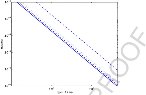
Fig. 1. Test problem. Efficiency plot. Box method solid line, Lax–Wendroff method dotted line, AGN dotted-dashed line, SGN dashed line.

The second step is to derive the values ofC1

,

C2

,

C3

,

aandbin the error and cost expressions(2.1)and(2.2). For this 1

issue, we have used a multiple regression technique. We compute such constants with the Matlab© routine

regress

. Also, 2

it providesR2(coefficient of determination which represents a quantitative measure of how well the fitted model predicts 3

the dependent variable: ifR2

=

1, then the fit of the model is perfect). InTable 5, we present the analytical approximations 4

to the global error and the computational cost (withR2_{higher than 0.99), and the optimal value ofr provided by(2.6).} 5

These approximations show us that the error caused by the size-discretization is higher than the error caused by the time-6

discretization. This fact could be explained by the existence of nonlinearities based on nonlocal terms. With respect to the 7

computational cost, there is an equilibrium between the size and time discretization unless the integration with the AGN 8

method which shows a higher dominance of the time discretization due to the accumulation of grid nodes. 9

InFig. 1we present the corresponding efficiency plot, where we display the error (in the vertical axis) and the work 10

(in the horizontal axis) in logarithmic scale. We choose for each method the value ofrthat represents the most efficient 11

∧

behavior, unless for the Lax–Wendroff method which also must satisfy the ∧

Courant–Friedrichs–Lewy(CFL) condition [15], 12

r

<

9

.

09. We obtain in such figure that the difference methods behave better than characteristics curves methods on the 13

error interval shown. The most efficient method correspond with the Lax–Wendroff method although the box method slope 14

is the best. Also it is shown that the selection procedure improves the ∧

behaviorof the characteristic curves methods. 15

Remark 1. Numerical experiments confirm the proposed expression for the computational cost formula(2.2). 16

Remark 2. Again, numerical experiments corroborate expression(2.1)for the global error. However, such formula would 17

a nonlinear least-squares fitting technique (into Matlab© is developed with

lsqcurvefit

function) which provides a 1

similar procedure. 2

Remark 3. Again, we have to point out that constants in formulae(2.1)and(2.2)depend on the specific problem being 3

approximated: functions data chosen, size of the time integration considered, etc. 4

3. Real data case: mosquitofish population 5

In this section, we deal with the evolution of a mosquitofish population described in [16]. The size interval is

[

9

,

63

]

and 6 we use the following

∧

functiondata: the fertility rate,

α(

x

,

t

)

=

α(

x

)

T_α

(

t

)

, where

α(

x

)

fitted to field data and 7

T_α

(

t

)

=





































t 30



3



1

−

t

−

30

10

+

(

t

−

30

)

2 150



,

for 0

≤

t

≤

30

,

1

,

for 30

≤

t

≤

90

,

−



t

−

120

30



3



1

+

t

−

90

10

+

(

t

−

90

)

2 150



,

for 90

≤

t

≤

120

,

0

,

for 120

≤

t

≤

365

,

8

the growth rateg

(

x

,

t

)

=

g

(

x

)

Tg

(

t

),

g

(

x

)

=

₈₀63_.2



1

−

x 63



,

9

≤

x

≤

63, and 9

Tg

(

t

)

=



































0

.

2

+

0

.

8



t

30



3



1

−

t

−

30

10

+

(

t

−

30

)

2 150



,

for 0

≤

t

≤

30

,

1

,

for 30

≤

t

≤

90

,

0

.

2

−

0

.

8



t

−

120

30



3



1

+

t

−

90

10

+

(

t

−

90

)

2 150



,

for 90

≤

t

≤

120

,

0

.

2

,

for 120

≤

t

≤

365

,

10

the mortality rate

µ(

x

,

z

,

t

)

=

µ(

x

,

z

)

T_µ

(

t

)

, 11

µ(

x

,

z

)

=































0

.

1 exp



₋

2000

z



,

for 9

≤

x

≤

31

,

0

.

1 exp



₋

2000 z



+



0

.

023

−

0

.

1 exp



₋

2000

z



(

x

−

31

)

3

(

1

−

3

(

x

−

32

) (

65

−

2x

)),

for 31

<

x

≤

32

,

0

.

023

,

for 32

<

x

≤

63

,

12

with

γ

_µ

(

x

)

=



₂, ₉≤x≤30,

−2(x−31)3(1+3(x−30) (2x−59)), 30<x<31, 0, 31≤x≤63.

13

T_µ

(

t

)

=































2

−



t 30



3



1

−

t

−

30

10

+

(

t

−

30

)

2 150



,

0

≤

t

≤

30

,

1

,

30

≤

t

≤

90

,

2

+



t

−

120

30



3



1

+

t

−

90

10

+

(

t

−

90

)

2 150



,

90

≤

t

≤

120

,

2

,

120

≤

t

≤

365

.

14

The numerical integration was carried out on the time interval

[

0

,

365

]

(1 year). For this real situation, a theoretical solu- 15 tion is unknown so, for the analysis developed in the previous section, we take, for each numerical method, the numerical 16 approximation computed on the finest grid as a representation of the exact solution. More precisely, we have employed 17 different values of the size and time discretization parameters and we choose the finest grid values as the solution

(

k

=

18 h

=

7

.

813E

−

3

)

. We present the results onTables 6–9, for the Lax–Wendroff, Box, AGN and SGN methods respectively. The 19 results in the tables clearly confirm the expected second order of convergence for such methods. We have to note that, in 20

Table 6, we show how the Lax–Wendroff method is not able to obtain the solution of the problem when the CFL condition, 21

r

<

1

.

485, is not satisfied. 22

With the same procedure used in the previous section, we can describe the expressions of the principal error terms and 23 computational cost with respect to the discretization parameters and the optimal value ofr, for each method, as shown in 24

Table 10, withR2higher than 0.98. The ∧

behaviorof the dominant error is as in the theoretical test example unless in the case 25

Table 6

Mosquitofish problem. Errors, CPU time (seconds) and order for Lax–Wendroff method.

k\h 1.250E−1 6.250E−2 3.125E−2 1.563E−2 1.250E−1 2.386E−04

2.16

6.250E−2 2.428E−04 5.883E−05 4.31 8.56 2.02

3.125E−2 2.441E−04 5.982E−05 1.410E−05 8.61 17.13 2.02 34.19 2.06

1.563E−2 2.446E−04 6.017E−05 1.444E−05 3.094E−06 17.33 34.51 2.02 68.77 2.05 138.93 2.19

Table 7

Mosquitofish problem. Errors, CPU time (seconds) and order for the Box method.

k\h 1.250E−1 6.250E−2 3.125E−2 1.563E−2

1.250E−1 2.049E−04 5.432E−05 2.544E−05 2.097E−05

5.47 10.75 21.88 43.30

6.250E−2 2.025E−04 5.088E−05 1.306E−05 6.189E−06 10.44 20.34 2.01 40.78 2.06 83.90 2.04 3.125E−2 2.022E−04 5.020E−05 1.203E−05 2.750E−06

20.10 39.47 2.01 78.39 2.08 160.86 2.25 1.563E−2 2.022E−04 5.020E−05 1.203E−05 2.750E−06

38.75 76.17 2.01 152.76 2.06 313.28 2.13

Table 8

Mosquitofish problem. Errors, CPU time (seconds) and order for the AGN method.

k\h 1.250E−1 6.250E−2 3.125E−2 1.563E−2 1.250E−1 2.854E−05 2.854E−05 2.854E−05 2.854E−05

6.20 7.90 11.29 18.72

6.250E−2 7.220E−06 7.220E−06 7.220E−06 7.220E−06 21.91 25.62 1.98 33.09 1.98 48.59 1.98 3.125E−2 1.891E−06 1.891E−06 1.891E−06 1.891E−06

86.54 94.17 1.93 109.61 1.93 141.13 1.93 1.563E−2 9.283E−07 9.283E−07 9.283E−07 9.283E−07

356.52 372.65 1.03 405.10 1.03 470.83 1.03

Table 9

Mosquitofish problem. Errors, CPU time (seconds) and order for the SGN method.

k\h 1.250E−1 6.250E−2 3.125E−2 1.563E−2 1.250E−1 1.653E−04 5.707E−05 2.991E−05 2.819E−05

1.58 3.14 6.35 12.92

6.250E−2 1.740E−04 3.858E−05 1.031E−05 7.220E−06 3.17 6.30 2.10 12.56 2.47 25.44 2.05 3.125E−2 1.435E−04 4.748E−05 8.595E−06 2.750E−06

6.35 12.64 1.87 25.16 2.17 50.27 1.91 1.563E−2 1.368E−04 2.984E−05 1.097E−05 1.788E−06

12.71 25.32 2.27 50.52 2.11 100.85 2.27

Table 10

Mosquitofish problem. Analytical approximations of global error and computational cost, and optimalr. Error Computational cost ropt

Lax–Wendroff 1.3E−02h2_+4.9E−04k2 _3.4E−02h−0.99_k−0.99 _5.19

Box 1.2E−02h2_+1.1E−03k2 _1.1E−01h−0.98_k−0.92 _3.30

AGN 2.8E−05h2_+2.1E−03k2 _1.3E−01h−0.37_k−1.68 _0.25

SGN 1.2E−02h2_+2.2E−03k2 _2.6E−02h−1.00_k−0.99 _2.27

Then we compare all the methods in the corresponding efficiency plot,Fig. 2, in which we use the optimalrfor all the 1

methods unless the Lax–Wendroff method which is limited by the CFL condition. The results confirm that the Box method 2

is the most efficient and that the SGN is the most efficient into the characteristics methods. These conclusions are different 3

from the ones given in [16]. In such work, we did not use the analytical expressions of the optimalrobtained in this work. 4

Finally, we want to add two aspects that we pointed out in [16]. The use of the finite difference methods introduces 5

Fig. 2. Mosquitofish problem. Efficiency plot. Box method solid line, Lax–Wendroff method dotted line, AGN dotted-dashed line, SGN dashed line.

perform solutions that fit the qualitative ∧

behaviorbetter than the finite difference methods. On the other hand, the long- 1 time integration shows some weakness in the numerical integration with the AGN method and makes more efficient the 2

SGN method because of the selection procedure. 3

4. Conclusions 4

We have presented a procedure to obtain an analytical approximation to the efficiency. We have used it to compare four 5 different second-order numerical methods. We have shown the best relation between the discretization parameters for each 6 method and we have obtained the most efficient numerical method in two situations: a theoretical example and other one 7 based on biological data. We have limited our study to these second order techniques, however other numerical procedures 8

would be considered. 9

Such comparisons ∧

dependstrongly on the problem analyzed, so, we cannot expect for a numerical method which behaves 10 better in all the possible numerical tests. Thus, for a particular problem, in which we usually have to compute numerically 11 the solution with many different data, the most efficient method seems to be the most useful and here we establish an 12

appropriate technique in order to compare them. 13

However, previous works [16] showed that not only the accuracy of the numerical approximations is an influential fact 14 but other qualitative properties are also necessary. At least, we expect the numerical integration provides a non-negative 15 approximation because the problem is biologically meaningful and they must keep the singularities the vital functions could 16 present and not to introduce other misunderstandings in the solution as, for example, spurious oscillations. 17 In general, on a long time integration, the use of methods which preserve some of the qualitative properties of the solution 18 can perform better. In this way, characteristics curves methods would be good candidates. Qualitative considerations should 19

be incorporated to select a particular numerical method for a specific problem. 20

Acknowledgments 21

This work was supported in part by the project of the Ministerio de Ciencia e Innovación MTM2011-25238 and the project 22

of the Consejería de Educación, JCyL VA191U13. 23

The authors are very grateful to the anonymous referees for their careful reading and their valuable aid to improve the 24

manuscript. 25

Appendix. Numerical methods 26

A.1. The Lax–Wendroff method 27

LetJbe a positive integer. Let the points of the grid in the size variable bexj

=

xmin

+

j h

,

0

≤

j

≤

J, whereh

=

xmax−x_J min 28

is the grid diameter. We denote bykthe time step, and the discrete time levels astn

=

n k

,

0

≤

n

≤

N

,

N

=



_T

k



approximation tou

(

xj

,

tn

)

, 0

≤

j

≤

J

,

0

≤

n

≤

N. We ∧

supposethat an approximation to the initial condition(1.3),U0_{, is} 1

given (for example, the grid restriction of the initial datau0). 2

The Lax–Wendroff method is a two-stage scheme defined for eachn

=

0

,

1

, . . . ,

N

−

1. First we calculate the intermediate 3

values in the following way 4

Un+

1 2 j−1₂

=

U

n j−12

−

k

2h



g_jnU_jn

−

g_j−n₁U_j−n₁



−

k

2

µ

n j−12

Un

j−12

,

(A.7) 5

where ∧

gn

j

=

g



xj

,

Qh



γ

gUn



,

tn



,

j

=

0

,

1

, . . . ,

J

;

x_j−1 2

=

1 2



xj−1

+

xj



,

Un

j−1₂

=

1 2



Un j−1

+

Ujn



, µ

n

j−1₂

=

µ



x_j−1 2

,

6

Qh



γ

µUn



,

tn



,

j

=

1

,

2

, . . . ,

J. The functionQh

(

Vn

),

n

=

0

,

1

, . . . ,

N

−

1, denotes the composite trapezoidal quadrature

7

rule and products

γ

_sUn

_,

_s

₌

_µ,

_{g, must be interpreted componentwise. In the second stage, we obtain the valuesU}n+1

j

,

j

=

8

1

,

2

, . . . ,

J

−

1, as 9

U_jn+1

=

U_jn

−

k

h



gn+

1 2 j+12

Un+

1 2 j+12

−

gn+

1 2 j−12

Un+

1 2 j−12



−

k

µ

n+

1 2 j U

n+1₂ j

,

10

U_Jn+1

=

0

,

11

where ∧

Un+

1 2

j

=

12



Un+

1 2

j+1₂

+

U n+1₂

j−1₂



, µ

n+1₂

j

=

µ



xj

,

Qh



γ

µUn+

1 2



,

tn

+

k₂



,

j

=

1

,

2

, . . . ,

J

−

1

;

gn+

1 2

j+1₂

=

g



x_j+1 2

,

12

Qh



γ

gUn

+1₂



_,

tn

+

₂k



,

j

=

0

,

1

, . . . ,

J

−

1. Now,Qh

(

Vn+ 1

2

),

₀

≤

n

≤

N

−

1, denotes the composite mid-point quadrature 13

rule. Finally, the approximationU₀n+1tou

(

xmin

,

tn+1

)

, for 0

≤

n

≤

N

−

1, is calculated with the condition 14

g₀n+1U₀n+1

=

Qh

(

α

n+1Un+1

),

15

whereg₀n+1

=

g



xmin

,

Qh



γ

gUn+1



,

tn



and

α

n+_j 1

=

α(

xj

,

Qh



γ

αUn+1



,

tn+1

),

j

=

0

,

1

. . . ,

J

,

0

≤

n

≤

N

−

1. Again, the 16

products

α

n+1_Un+1_and

_γ

sUn+1

,

s

=

g

, α

, must be interpreted componentwise.

17

A.2. The Box method 18

The parametersJ

,

N

,

handk, and also the mesh grid, are defined as inAppendix A.1. Again, we start with an initial 19

conditionU0_. 20

We introduce the half integer grid pointsx_j−1 2

=

1 2



xj−1

+

xj



,

1

≤

j

≤

J; the mean value operators ∧

Un+

1 2 j

:=

1 2



U_jn+1

+

21

Un j



,

Un

j−1₂

=

1 2



Un j−1

+

Ujn



,

Un+

1 2

j−1₂

=

1 2



Un+

1 2

j−1

+

U

n+1₂ j



and the difference operatorD Un j

=

U

n+1

j

−

Ujn.

22

The box method is defined by 23

D U_jn

+

D U_j−n₁

2k

+

gn+

1 2

j U

n+1₂ j

−

g

n+1₂ j−1 U

n+1₂ j−1

h

= −

µ

n+1₂

j−1₂ U n+1₂

j−1₂

,

(A.8)

24

g₀n+1U₀n+1

=

Qh

(

α

n+1Un+1

),

(A.9)

25

1

≤

j

≤

J

,

0

≤

n

≤

N

−

1, whereQh

(

Vn

)

represents the trapezoidal quadrature rule, and, for 0

≤

n

≤

N

−

1:g n+1₂

j

=

26

g



xj

,

Qh



γ

gUn+ 1 2



,

tn

+

k₂



,

0

≤

j

≤

J

,

g₀n+1

=

g



xmin

,

Qh



γ

gUn+1



,

tn+1



; ∧

µ

n+1₂

j−1₂

=

µ



x_j−1 2

,

Qh



γ

µUn+

1 2



,

tn

+

k₂



,

27

1

≤

j

≤

J. Notation for

α

n_{as in the Lax–Wendroff method.}

28

A.3. Aggregation grid nodes method (AGN) 29

The parametersJ

,

N

,

handkare defined as inAppendix A.1. 30

The initial grid nodes are given byX_j0

=

xmin

+

j h

,

0

≤

j

≤

J. We suppose that the approximations to the theoretical 31

solution in such nodes are known,U0

j

,

0

≤

j

≤

J. We also suppose that at the first time levelt1, the new grid nodes,X1, and 32

the corresponding solution values,U1_{, are known. Furthermore,X}0

j andX

1

j+1

,

0

≤

j

≤

J

−

1, are (numerically) in the same 33

characteristic curve. Angulo and López-Marcos obtained the initial conditions by means of the well-known second order 34

method [13]. 35

The numerical approximations at the time leveltn+2

,

0

≤

n

≤

N

−

2 are obtained as follows. We suppose that the nu-36

merical approximations at the previous time levels,tnandtn+1, are known,Xn

,

UnandXn+1

,

Un+1. WhereXjnandX n+1

j+1

,

0

≤

37

j

≤

J

+

n

−

1 belong (numerically) to the same characteristic curve. We introduce the notation

µ

∗

₍

_x

_,

_I

g

(

t

),

Iµ

(

t

),

t

)

=

µ(

x

,

Ig

(

t

),

Iµ

(

t

),

t

)

+

gx

(

x

,

Ig

(

t

),

t

),

Q

(

X

,

V

)

=



p−1

j=0

Xj+1−Xj

2

(

Vj

+

Vj+1

)

;

(

γ

s

)

j

=

γ

s

(

Xj

),

s

=

α,

g

, µ,

j

=

0

,

1

, . . . ,

p. This 1 notation will be used throughout the subsection. First, the grid values at the time leveltn+2are calculated by 2

X₀n+2

=

xmin

,

XJ+n+n+22

=

xmax

,

(A.10) 3

X₁n+2

=

X₀n+1

+

k g



X₀n+1

+

k 2g



X₀n+1

,

Q



Xn+1

_,

_γ

gUn+1



,

tn+1



,

3Q

(

Xn+1

_,

_γ

gUn+1

)

−

Q

(

Xn

,

γ

gUn

)

2

,

tn+1

+

k

2



,

(A.11) 4

X_jn+2

=

X_j−n₂

+

2k g

(

X_j−n+₁1

,

Q



Xn+1

,

γ

_gUn+1



,

tn+1

),

2

≤

j

≤

J

+

n

+

1

,

(A.12) 5

and the approximations to the theoretical solution in these nodes at such time level using 6

U₁n+2

=

U₀n+1exp



−

k

µ

∗



X₀n+1

+

k 2g

(

X

n+1 0

,

Q



Xn+1

,

γ

_gUn+1



,

tn+1

),

3Q

(

Xn+1

_,

_γ

gUn+1

)

−

Q

(

Xn

,

γ

gUn

)

2

,

3Q

(

Xn+1

_,

_γ

µUn+1

)

−

Q

(

Xn

,

γ

µUn

)

2

,

tn+1

+

k

2



,

(A.13) 7

U_jn+2

=

U_j−n₂exp



−

2k

µ

∗



X_j−n+₁1

,

Q



Xn+1

,

γ

_gUn+1



,

Q



Xn+1

,

γ

_µUn+1



,

tn+1



,

2

≤

j

≤

J

+

n

+

1

,

(A.14) 8

U_J+n+n+2₂

=

0

.

(A.15) 9

The equations at the time leveltn+2are completed with the approximationU0n+2tou

(

xmin

,

tn+2

)

by means of the discretiza- 10

tion of the boundary condition(1.2) 11

U₀n+2

=

Q

(

X

n+2

_,

_α

₍

_Xn+2

_,

_Un+2

₎

_Un+2

₎

g

(

xmin

,

Q



Xn+2

,

γ

gUn+2



,

tn+2

)

,

(A.16) 12

where

α

j

(

Xn+2

,

Un+2

)

=

α



X_jn+2

,

Q

(

Xn+2

_,

_γ

αUn+2

),

tn+2



,

0

≤

j

≤

J

+

n

+

2

,

0

≤

n

≤

N

−

2.

Q2 13

A.4. Selection grid nodes method (SGN) 14

The following scheme considers a modification in the grid of the previous one so that, by using a selection of the grid 15 nodes, the number of nodes does not increase at each time level. Thus, we try to reduce the computational cost without loss 16

of accuracy. 17

The grid nodes and the numerical approximations at timet2

,

X2

,

U2, are defined by means of(A.10)–(A.16)forn

=

0. 18 Next, we calculateQ2

₍

_X2

_,

_γ

2

µU2

)

. 19

At the new time level, there is a different number of nodes because a new node that fluxes through the boundary is 20 introduced. So, at the time levelt0, we have

(

J

+

1

)

grid nodes, att1we have

(

J

+

2

)

and att2we have

(

J

+

3

)

. Now, the first 21

grid nodeX_l2that satisfies 22

|

X_l+2₁

−

X_l−2₁

| =

min 1≤j≤J+1

|

X_j+2₁

−

X_j−2₁

|

23

is eliminated and, alsoX1

l−1, the grid node in the same characteristic curve att1, is taken out. The number of nodes at the 24 levels involved in the implementation of our two-step scheme are kept fixed:

(

J

+

3

)

nodes for the time level reached in the 25 integration and

(

J

+

2

)

and

(

J

+

1

)

for the previous ones. However, the approximations to the nonlocal terms at such time 26

levels are not recomputed. 27

Now, we suppose that the numerical approximations at time levels tn and tn+1 are known, and they are denoted 28 by



Xn

0

,

X1n

, . . . ,

XJ−n1

,

XJn

=

xmax



,



Un

0

,

U1n

, . . . ,

UJ−n1

,

UJn

=

0



,

Q

(

Xn

_,

_γ

sUn

),

s

=

α,

g

, µ

, and_∧

{

Xn

+1

0

=

xmin

,

X1n+1

, . . . ,

29

X_Jn+1

,

X_Jn₊+₁1

=

xmax

}

,



U₀n+1

,

U₁n+1

, . . . ,

U_Jn+1

,

U_Jn₊+₁1

=

0



,

Q

(

Xn+1

_,

_γ

sUn

+1

_),

_s

₌

_α,

_g

_{, µ}

_{(note thatX}n j andX

n+1

j+1

,

0

≤

j

≤

30 J

−

1, are, numerically, in the same characteristic curve). In addition, the grid considered attnhas lost two nodes with respect 31 to the moment whenXn_{was actually calculated, while the grid used att}

n+1has only one node less thanXn+1. The numerical 32 grid nodes at the new time leveltn+2, are computed by means of(A.10)–(A.12), 2

≤

j

≤

J

+

1, and the approximations to the 33 theoretical solution in these nodes are obtained using(A.13),(A.14), 2

≤

j

≤

J

+

1, and(A.15). The equations at time leveltn+2 34 are completed with the approximationU₀n+2tou

(

xmin

,

tn+2

)

using(A.16). Now, we calculateQ

(

Xn+2

,

γ

sUn+2

),

s

=

α,

g

, µ

. 35

Note that, for the time levelstn

,

n

≥

2, the quadrature rules always use the same number of nodes

(

J

+

3

)

. Finally, we 36

eliminate the first grid nodeX_ln+2that satisfies 37

|

X_l+n+₁2

−

X_l−n+₁2

| =

min 1≤j≤J+1

|

X_j+n+₁2

−

X_j−n+₁2

|

38

References

1

[1] J.A.J. Metz, E.O. Diekmann (Eds.), The Dynamics of Physiologically Structured Populations, in: Springer Lecture Notes in Biomathematics, vol. 68, Springer, Heildelberg, 1986.

2

[2] J.M. Cushing, An Introduction to Structured Populations Dynamics, in: CMB-NSF Regional Conference Series in Applied Mathematics, SIAM, 1998.

3

[3] B. Perthame, Transport Equations in Biology, Birkhäuser Verlag, Basel, 2007.

4

[4] A. Calsina, J. Saldaña, A model of physiologically structured population dynamics with a nonlinear individual growth rate, J. Math. Biol. 33 (4) (1995) 335–364.

5

[5] N. Kato, A general model of size-dependent population dynamics with nonlinear growth rate, J. Math. Anal. Appl. 297 (2004) 234–256.

6

[6] A.S. Ackleh, M.L. Delcambre, K.L. Sutton, D. Ennis, A structured model for the spread of mycobacterium marinum: foundations for a numerical approximation scheme, Math. Biosci. Eng. 11 (2014) 679–721.

7

[7] A.S. Ackleh, K. Deng, K. Ito, J. Thibodeaux, A structured erythropoiesis model with nonlinear cell maturation velocity and hormone decay rate, Math. Biosci. 204 (2006) 21–48.

8

[8] O. Angulo, R. Bravo de la Parra, J.C. López-Marcos, M.A. Zavala, Stand dynamics and tree coexistence in an analytical structured model: the role of recruitment, J. Theoret. Biol. 333 (2013) 91–101.

9

[9] L. Abia, O. Angulo, J.C. López-Marcos, M.A. López-Marcos, Numerical integration of a hierarchically size-structured population model with contest competition, J. Comput. Appl. Math. 258 (2014) 116–134.

10

[10] O. Angulo, J.C. López-Marcos, M.A. López-Marcos, Analysis of an efficient integrator for a size-structured population model with a dynamical resource, Comput. Math. Appl. 68 (2014) 941–961.

11

[11] L. Abia, O. Angulo, J.C. López-Marcos, Size-structured population models and their numerical solutions, Discrete Contin. Dyn. Syst. Ser. B 4 (2004) 1203–1222.

12

[12] O. Angulo, J.C. López-Marcos, Numerical integration of autonomous and nonautonomous nonlinear size-structured population models, Math. Biosci. 177 (2002) 39–71.

13

[13] O. Angulo, J.C. López-Marcos, Numerical integration of fully nonlinear size-structured population models, Appl. Numer. Math. 50 (2004) 291–327.

14

[14] S.F. Goldsmith, A.S. Aiken, D.S. Wilkerson, Measuring empirical computational complexity, Proc. ESEC/FSE (2007) 395–404.

15

[15] K.W. Morton, D.F. Mayers, Numerical Solution of Partial Differential Equations, Cambridge University, Cambridge, 1994.

16

[16] O. Angulo, A. Durán, J.C. López-Marcos, Numerical study for size-structured population models: a case ofGambussia affinis, C. R. Biol. 328 (2005) 387–402.