Dynamic Soil-Structure Interaction in Bridge Abutments

(1)

DYNAMIC SOIL-STRUCTURE

INTERACTION IN

BRIDGE ABUTMENTS

**A. Martinez*, J.**

Mateo~

and E. Alarcon*

m

Advances in Boundary Element Methods Civil-Comp Press, Edinburgh, 135- 14J

*

Department of Structural Mechanics and Industrial Constructions,

Technical University of Madrid, Madrid, Spain

~universidad

Pontificia Coomillas, Madrid, Spain

Abstract

Strong motion obtained in instrumental short-span bridges show the importance of the abutments in the dynamic response of the whole structure. Many models ha ve heen used in order to take into account the influence of pier foundations although no reliable ones have been used to analyse the abutment performance. In this work three-dimensional Boundary Element models in frecuency domain have been proposed and dimensionless dynamic stiffness of standard bridge ahutmcnts have been obtained.

1 Introduction

The study of the dynamic response of bridges, specially to seismic actions, has reached a great interest because the amount of bridge failures which have happened in recent earthquakes: Loma Prieta (1989), Northridge (1994), Kohe (1995).

Among many other aspects soil structure interaction is a very important aspect to be taken into account in the dynamic modelling of those structures. Many studies have asses numerically the soil-structure phenomena: Ma-Chi Chen and J. Penzien 0979) [2], D.R. Somaini (1984) [14], J.P. Wolf (1985) [22], Spyrakos (1990) [15], [16] and E. Maragakis (1989) [8]. In the same sense, studies based on the response of instrumented structures to seismic actions require to take into account large concentrated damping factors to include those effect11 using system identification techniques: C.B. Crouse, B. Hushmad and G.R. Martín (1987) [3], J.C. Wilson (1986) [19], S.D. Wemer, J.L. Beck and M.B. Levine [18].

These studies pointed out the importance of soil-structure interaction effects both in pier foundations and abutments. As techniques similar to those used in other kind structures may be employed in pier foundations, we are going to focus only in the af?utments effects which largely depend on deck-abutment connection and their tipology:

• In decks simply supported on the abutments these effects

are small because the elastomeric bearings act as seismic isolators.· However the deck might contact the abutment if seismic buffers are installed; they may act also when the displacements are greater than a prefied value or because the expansion joint between the deck and the ahutment i11 not dimensioned to absorved the induced dynamic displacements.

• In short span bridges and undercrossing structures in urban areas, the portal effect may be used in order to reduce the stresses in the abutments, taking the horizontal loads through the bridge deck from one abutment to the other one. In those cases, the knowledge of the stiffnes properties of the soil-abutment system is required.

• The use of integral abutments, in which the deck is monolithic with the abutments, causes a saving in both installation and maintenance of the expansion joinK Displacements due to thermal and theoretical deformations are released through the flexibility of the soil-abutment system usually founded on piles.

• In long span bridges with high piers subjected to strong

horizontal accelerations due to live loads, like in railway bridges, or to seismic actions, the deck can be fixed to one of the abutments in order to reduce the stresses on the piers.

The studies carried out by J.C. Wilson and B.S. Tan [20], [21], include a frrst attempt to make a simplified representation of the approaching embankments and present numerical values of the damping and stiffness that would be necessary to understand the values registered in an actual instrumented structure.

This study will show the evaluation of the dynamic stiffnesses in two and three dimensional abutments and their application to the dynamic behavior of bridges. It will summarize our attempt to apply well known techniques to solve a new problem: E. Alarcón et al. [1], A.M. Cutillas et al. [9], [10], [11], [12], [13].

Fundamental Soil-structure Interaction equations will he formulated and Boundary Element Method will be applied to obtain, for both cases, the stiffnesses as a function of dimensionless variables in the frequency domain.

2 Dynamic soil-structure interaction

2.1 Formulation

(2)

For both the soil an the structure an elastic or linear viscoelastic behavior will be assumed.

For convenience, in soil subdomain the situation prior to the structure construction will be refered as free field and thc excavation subdomain will be that part occupied hy the structure.

®

r---,

l

I

V'

1 1

L - - -

~~-

- - - _¡

1

Oz

r---,

:~

al

.. 'D

_{¿J ..}

r

~

•• 1

•a

L - - - ~~- - - _j

@

r---,

o.

:~

¡/:

1 Os

r 1

L - - - ~~- - - _1

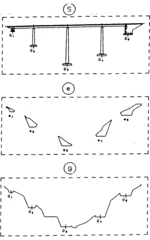
Figure 1: Soil and bridge structure subdomain

The numerical treatment mak:ing use of Finite Element or Boundary Methods requires the discretization of these domains. The node notation will be as usual [22].

Subscripts have the following meanings:

s: nodes belonging only to the structure b: soil-structure interface nodes g: soil domain with excavation f: soil domain without excavation e: excavated soil domain

Fig. 1 shows the subdomains in the case of a bridge structure.

The equations of motion in the discretized domain Q can

be formulated in the frecuency domain:

[ -ro2 M+

iroC

+K ]u(ro)

=

P(ro)

S(ro)u(ro)

=

P(ro)

(2)

where:

S(ro)

=

-ro2 M+ iroC +K= Kest (K*+ iroC*) (3)

is the dynamic stiffness matrix, or impedance matrix.

2.2. S obstructores method. Equations of motion

The most widely used technique in linear interaction prohlems in

the so called Substructure method. Due to the different characteristics of the soil and structure domains, it is useful to obtain the dynamic stiffness for both of them independently and, later on, to perform a coupled analysis.

This approach allows the use of different discretizations and different analytical and numerical techniques in each subdomain.

According to eq.2, and the dynamic equilihrium equations in the structure and soil domain and the compatibi1ity equations at the interface, the complete soil-stn·:;ture equations are:

(4)

Where

(5)

is the total displacements and s~b is the dynamic stiffness matrix of the structure for the nodes in contact with the soil,

ug

is the

ground motion without the structure and s~b is the dynamic stiffness matrix of the soil.

Those equations point out the three steps in which every soil-structure interaction problem may be studied:

• Step 1: Soil motion calculation at the foundation leve!, or at the soil-structure interface

u

8• Such motion can be

obtained using the known surface motion, by means of a deconvolution process or based on the scattered motion calculation from the known motion far away from the surface.

• Step 2: Dynamic stiffness analysis of the soil S~, that is of the free soil surface plus the indentations produced by the foundation excavations.

• Step 3: Analysis of the structure once the dynamic stiffness matrix obtained in step 2 has been added and suhmitted to the motion obtained in step l.

These equations may be simplified when a rigid foundations, is assumed. The degrees of freedom at the interface nodes are reduced to six times the number of supports, if

multiple support excitation is considered or to only six degrees of freedom if the same motion is considered in all the supports.

3 Boundary Elements Method

The Boundary Element Method, B.E.M. is one the most powerful techniques to analyze dynamical problem.s in unbounded continuum media like those involved in soil-structure interaction phenomena.

The method applies discretizing techniques to the integral formulation of Elastodynamic Problems obtained from the Dynamic Reciproca/ Theorem and the Fundamental Solutions, [4], [7].

(3)

Classical Betti' s Reciproca! Theorem of elastostatics was obtained for elastodynamic by D. Graffi in 1946-1947, and further extended to unbounded domains by Wheeler and Stemberg in 1968.

If two different Elastodynamic States are considered:

(6)

where U¡, t¡ and b¡ are the displacements, tractions and body forces vectors respecti vely.

Let Q be a regular region with boundary

r

=

an.

The Reciproca! Theorem in the frecuency domainis:

where the variables represent their arnplitude in the steady-state situation.

3.2. Integral equations

The reciproca! theorem will be applied taking the actual elastodynamic as EA and being EB that corresponding to a unit concentrated impulse load following direction i:

(X)

where O is the Dirac's delta distribution

For the EB state, zero initial conditions are prescribed. The corresponding displacements and tractions may be written as:

where the expresions for Uii and Tii are known. The following integral equations are obtained:

C(s)u¡ (s;ro)

=

fru

₉(x.s;ro)tj

(x;ro)dr-- fr _T9(x,s;ro)uj (x;ro)dr

+

(9)

+

p

J.a

U !i (x,

s;

ro) b j ( x; ro) dQ (1 O)

where:

¡

IifsEn

C(S)

=

i

if S E

r

with smooth on

s

O if

S

E Qc

nc

is the complement of

n,

the domain considered.

3.3. Integral equations discretization

(11)

The Boundary Elements Method applies the robust

domain discretization and variable interpolation techniques from Finite Elements Method to the solution of integral equations 1 O.

In

frecuency domain equations, only the discretization of the geometrical variables is required.

The boundary, in 3-D domains, will be discretized inta surface elements. The domain will be discretized inta salid elements whcih actually are integration cells.

The discretization of the integral equations leads ta a linear system of equations:

Hu· Gt=F (12)

Where u and t are the displacements and traction vectors at the boundary, respectively.

If the body forces are not considered, the matrix equation will be reduced to:

Hu=Gt (13)

to salve every mixed boundary value problem.

4 Dynamic stiffness analysis

The dynamic-stiffness matrix evaluation af the sail

s;b

i.c; the second step in every soil-structure analysis. It is necessary ta salve the mixed boundary value problem in the subdomain Og where the displacements are known in part or total soil-structure interface, (d0u) and in the rest of the boundary (aQt) tractions are null.

If a flexible contact between soil and structure is considered it will be necessary to salve such boundary value problems in as many nades

as

degrees of freedom exist at the interface. In a rigid contact case, the displacements and the resultant of stresses may be referred to a characteristic point. The number of boundary value problems ta be solved are equal to the total number of foundations times the number of degrees of freedom considered.

Recent strong motion records obtained in instrumented short span bridges show the importance of the abutments in the dynamic response of the whole structure.

Sorne models have been proposed in arder to evaluate the dynamic influence of the abutments. Surprisingly they are very different to those used in the analysis of surface foundations.

J.C. Wilson and B.S. Tan (1990) [20], [21] show an interesting study about the embankment-abutment influence in the seismic response of Meloland Road Overpass. In a first part of the study a 2D fmite element model is propased to abtain the vertical and horizontal static stiffness of the whole embankment-abutment and its natural frecuency.

With the experimental data and employing system identification techniques, an important reduction of embankment-abutment natural frecuency was detected and high damping ratios between 25 and 45% were identified. These concentrated damping radios represent modal damping ratios from 3 to 12% for certain modes in the whole structure.

Applicatian of Boundary Element Method to this

particular interaction problem will justify numerically the

results obtained experimentally [13].

4.1. Calibration models

In arder ta test the validity of B.E.M. the problems proposed by J.H. Wood (1973) [23] and H. Tajimi (1973) [17] were selected as benchmarks.

They are related to wall retaining structures both in bounded and unbounded damains; the second one is specially suited to be solved by B.E.M. techniques.

Those benchmarks allow the stablisment of discretization criteria for the solution of the new problems.

4.1.1. Wood's model

(4)

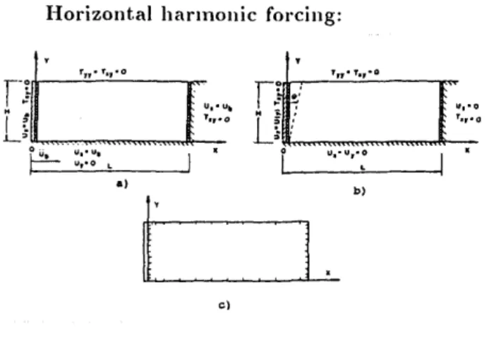
The upper horizontal boundary is a free one while the lower is fi«id. The vertical boundaries represent smooth rigid walls. A linear elastic behaviour of the soil is assumed.

Two forced solutions were analyzed: horizontal harmonic forcing on rigid boundaries and rotating harmonic forcing of a wall.

Horizontal hannonic forcing:

a)

b)

¡['

_{' : :1}

e)

figme 2: Wood's model

A horizontal harmonic displacement is imposed on the rigid horizontal boundary and on the vertical smooth rigid walls Fig.l.a. This horizontal displacement derive from a harmonic aceleration of the base. A constant aceleration in frecuency domain implies a frecuency dependent displacementc;; in this domain:

üb (t)

=

aeirol (14)

(15)

where a. is the constant amplitude of the aceleration and A( ro) i~

the frecuency dependent displacement amplitude.

a.

A( ro)=

-2

(l)

(16)

(17)

Dissipation effects were taken into account in W ood 's analysis by addition of viscous damping terms. These terms include non linear behaviour within the soil structure and the radiation of energy from the system owing to the fact that in general the boundaries are not perfectly rigid.

To duplicate the results a constant boundary element mesh was built. Special care must be taken with the corners to obtain accurate results Fig.l.c.

Dissipation effects are naturally taken into account in the viscoelastic formulation with an hysteretic damping coefficient.

Complex amplitude ratios of resultant forces and moment of the horizontal stresses behind the rigid wall against

dimensionless frecuency

n

=

~

are shown in Fig.3 ro in the

ros

angular frecuency of the imposed displacement; ros= n -Cs . IS

2H the natural angular frecuency of the lowest pure shear mode of

an

infinite

stratum, and c5 =

~

is the shear waves

propagation velocity.

Resultant forces and moments are normalized to the static ones.

L/H• 1.0

·ZD

a)

WOOD.

- • • O . S

-.·o•s

...

••O.J

'--'". s.o

b)

Figure ~l: Horizontal harmonic forcing: Complex amplitude ratios

1.0 0.8

; 06

z: 04

a)

- wooo. o l[t.l.

on 1.00 UD a:/[ 8

L/H• 1.0 ~·0.3

/"'l. • !O 1.0

- wooo.

0.8 o BEM. Y/H

.... 0.6

~

¡;;

z: 0.4

0.2

o.o '-0.0__.,10-2~.0 ----=,.0~40

IMV'IH US

b) o

8'1/[0

Figure 4: Rocking harmonic forcing: Stress distribution

Rocking harmonic forcing

In this case a rigid rotational deformation of the wall around its base is considered Fig.2.b.

Stress distribution behind the rigid wall both statical and dynamical case is shown in Fig.4 where it is seen that B.E.M. results agree with Wood's ones.

u,•o

Taa •O

.!... r,. '•r•o

TAJIMI'S PR08LEM

a)

Figure 5: Tajimi's model

4.1.2. Tajimi's Model

lE M MODEL.

b)

Tajimi obtained a solution for the harmonically forced wall problem in a quarter space using two-dimensional elastic wave propagation theory Fig.5.a. In the static case (excitation frequency equals to zero) his results agree with those ohtained by W.D.L. Finn (1963) [6].

The comparison with the B.E.M. model is shown in Fig.5.b.

Horizontal translation of the wall

The numerical results ot total pressure distrihution is

(5)

and the dimensionless frecuency rol-! , v ₅

=

c₅

=

{Q

for a

Vs

VP

velocity ratio of shear to longitudinal waves of

~

=

1 13 which

vP

correspond toa Poisson's ratio v = 0.4375.

The resultant force acting behind the wall can he determined from:

The good agreement between analytical (Tajimi's) and numerical results (B.E.M.) can be seen in Fig.6.a.

Rocking of the wall

The total pressure distribution in this case can he expresed as:

from:

The resultant moment about the bottom is determined

'•·'"'·''

·~·-.·.

~·o•

01 "

.,

•z'""'

lll,h .. U

1>)

·~·

1

.

1

o ':-0 =--~ •• - .. -"

-,.o--03 ~ 10

..-Fignre 6: Tajimi·s model. Stress distribution and resultant

with the )ame pararr ~ters used in the horizontal translation of the wall.

The results are shown in Fig.6.b.

Sorne considerations must be done about the B.E.M. mesh:

• Special care must be taken with corners. Small elementli of the same size must be employed around each one or special integral rules have to be implemented.

• There is a singularity in the stress field at the bottom of the wall so a careful discretization must be used.

• As two of the boundaries are unbounded, element mesh must be truncated in a sensible way to guaranteee the accuracy.

- In the static case (ro= 0), good results have been obtained for L/H = 20 and 50 constant elements.

- In the dynamic case (ro -:t: 0), good results have been

obtained with an adaptive mesh dependi}Jg on the frecuency with L = As /4 where As is the wave length for shear waves and the size of the element less than

As

/6.

4.2. Dynamic stifness of bridge abutments

Although the application fiel of two dimensional models is quite large, most of bridge abutments ha ve a three dimensional behaviour.

The abutment used in this study has a vertical front wall and two lateral walls perpendicular to the first one (Fig.7).

The main assumptions are:

• Linear viscoleastic behaviour of the soil whose main parameters are: density

p,

shear modulus G, Poisson 's

ratio

v

and damping ratio

~-• Rigid behaviour of the walls

Sorne special assumptions have been done about the abutment-embankment geometry in order to reduce the variables involved:

• The approach embankment, behind the wall, is considered

horizontal and unlimited. Next to the wall the grade of the

embankment is small because it is usually located in a vertical parabolic alinegment close to its vertex. The small

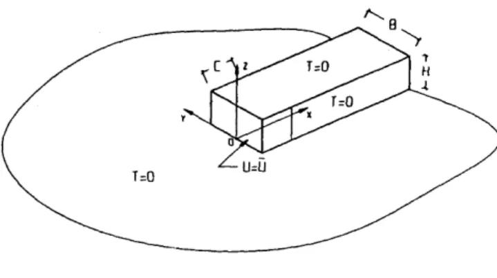
Figure 7:· Typical three dimensional abutment

grading produce embankment lengths from twenty to thirty times the wall height which can be considered unlimited for this purposes.

• The influence of the lateral slopes of the embankment has

not been considered. A granular type material is usually

employed to build the approach embankments so sorne planes and transition eones are needed to make them stable. As these parts of the embankments are not really well compacted, their capacity to resist an stress increment is very small. Ji is hoped that to neglect the slopes influence may not affect to the stiff component although it

(6)

• As a frrst approach to the problem the foundation of the walls have not been considered in order to isolate the wa1ls influence. The foundation have a big influence in the vertical component of the dynamic stiffness.

Under those assumptions the boundary value prohlem to

be solved is shown in Fig.8. The geometry is a rectangular prism on the halfspace which represent the approach emhankments with the following boundary conditions:

• The horizontal planes,

z

= O y

z

= H, are the free boundaries of the half space and the emhankment respectively. The tractions in those planes are null.

• The vertical plane

x

= O, is the plane contact between the embankment and the front wall of the abutmcnt. The displacements are known in order to evaluate the stifness of the system.

• The vertical planes y = B/2 y = -B/2 have both a contact with the lateral walls of the abutment, O S

x

< C. where the displacements are known and a free boundary

x

2 C.

T=O

Figure S: Boundary value problem

The structure of the dynamic stiffness matrix of the standard abutment, S&o

(ro),

may be expresed referred to the

coordinate system (O;XYZ) in the following way:

xz.

O Sy O Sy,xx O Sy,zz

S~ O Sz O Sz,yy O

Syy,x O Syy,z O Syy O

O Szz,y O Szz,xx O Szz

(22)

There are null terms because of the plane of symmetry

Direct stifnesses thet is, the main diagonal terrn will be specially studied, because the coupled stiffnesses have a less dominant role.

The stiffness terms may be expressed as usual:

S(ro)

=

K(ro) = Kst [k(ro)+ia₀c(ro)] (23)

with ao == roH 1 Cs

The variables involved in the discretization of the geometry like the free discretized surface and the characteristic size of the elements have been studied in [10]. The last one of these two variables is most important for the frecuency range studied. The different boundary element meshes used to compare the results are shown in Fig.9.

For the dimensionless ratios B/H

=

2 and C/H

=

1 the static stifnesses may be expressed as:

Kx =6.01 GH

2-v

K =4.90 GH

Y

2-v

K =6.08 GH

z

2-v

K = 5.69 GH

3

xx

2-v

K

=

5.10 GH

3

YY

2-v

GH3

Kzz

=9.27--2-v

(24)

The Poisson's ratio dependence of the dimensionless dynamic stiffness in the forrn (23), is shown in Figs.IO, 11 and 12, which are the longitudinal and transverse displacement~ and the rotation in a vertical plane.

The displacements stiffness components kx , ky and kz have a similar v dependence. For a dirnensionless frecuency ao less than 2 (ao < 2), there is not any Poisson's ratio dependence. For bigger values this dependence could be very important, specially for kx and kz components and great v values (v > 0.4)

The rotation stiffness cornponents kxx , kyy and kzz and all the damping components

e,

have a very homogeneus v dependent behaviour for the range of frecuencies studied. This dependence may be considered

n-1

n-3 n-2

(7)

k:r STIFFNESS

0.5 1.5 2 2.5 3

ao = wHjc.

- "= 0.00 -+- "= 0.10 --- "=0.20 -<r-V= 0.30 __.. V= 0.40 -+-V =0.50

ex STIFFNESS

ao = wHjc,

- v=O.OO -+-- V= 0.10 -+-V= 0.20 -<r- V= 0.30 _...., V= 0.40 -+- V= 0.50

Figure 10: Abutment on the half-space. Dynamic stiffnesses /\'.1'·

¡; dependence

This variation is similar to those obtained by Veletsos for

superficial circular footing [5]. . .

It is worth mentioning the decreasmg values m the stiffness components, even reaching negative values. Negati~e values show that inertial affects are larger than stiffness ones for such frecuencies.

As the real part of the dynamic stiffness is:

2

K(m) = R[S(m)] =K- m M (25)

for sorne m values the term

ai

M may be greater than K and the

dynamic stiffness will be negative. . .

In a different way, damping components have mcreasmg values with frecuency for the range studied.

5 Conclusions

The main conclusions of this work may be summarized as follows:

cy STIFFNESS

- v=O.OO -+- v=O.IO _.._ V =0.20 ao = wHjc_,

-<r-V= 0.30 ....,.._ V= 0.40 --+- V= 0.50

ky STIFFNESS

0.5 1.5 2 2.5 3

- V =0.00 -+- V= 0.10 -+- V= 0.20 ao=wH/cs

... "= 0.30 _...., V= 0.40 --+- V= 0.50

Fig1tn' 11: Abutment on the half-space. Dynamic stiffnesses l\·,1 · '' dependence

• High damping ratios have been detected in the dynamic response of instrumented structures subjected to strong seismic motion or subjected to forced motions in tield experiments. These values are obtained for special modes of response both in pier foundations and abutments. These modes of response may be produced by the contact between deck and abutment. This contact will be caused accidentally or by design requirements.

• Boundary Element Method (B.E.M.) is the most powerful technique in the analysis of dynamical prohlems in unbounded domains.

• Two dimensional calibration models have been employed to verify B.E.M. techniques agreement in earth retaining structures analysis.

• A three dimensional bridge abutment with frontal and lateral walls has al so been anal yzed.

The size of the elements employed in the discretization is the main parameter to be taken into account in a 3D mesh.

(8)

cyy STIFFNESS Cyy

0.7 ...---;---~---:--~--~

. 0.6 ···+··· ... ·r;;;¡· .. ·~"'"'t'(·¡;"'"'~·"'·~···

..

~· ~~~~~

o.s ···----····

71

0.4

0.3

0.2

0.1

o o

-:. -.. -... -....

~--

.. .. ... ...·r... .... ..

-... ¡

... ¡ ...

¡ ..

.... ~ .. -... -~ ... .

• • • • • • • • • • • • • ·:· • • • • • • • • • • • • • • • • • • ~-. • • • • • • • • • • • • -~-• • • • • • • • • • • • • • • • • • ~-o • • • • • • • • • • o • • • • • -~ • • • ' • • • • • • - • • • • • •

0.5 1.5 2 2.5 3

ao =-wHfc,

- V =0.00 --+- V= 0.10 -+-V= 0.20 -e-V= 0.J0 __,... V= 0.40 -+-11 =0.50

kyy STIFFNESS

0.5 1.5 2 2.5 3

- V =0.00 --+- V =0.10 -+-V= 0.20 ao = wHfc, -e-V= 0.30 - - V =0.40 -+-V= 0.50

Figun-• 1'2: Abutment on the half-space. Dyna mi e stiffnesses

1\_'₁_{" 1. ti}dependence

References

[1] Alarcón, E., Martínez, A., Gómez, M.S. "Dynamic stiffness of bridge abutments", Proc. 10th. World Conf on

Earth.Eng., Madrid, 1992

[2] Chen, M.C. Penzien, L. "Soil-structure interaction of short highway bridges" Proceedings of a Workshop on

Earthquake Resistance of Highway Bridges Applied

Technology Council. Pp 434 January 1979

[3] Crouse, C.B., Hushmand, B., Martin, G.R. "Dynamic soi1-structure interaction of a single-span bridge" Earth.Eng. &

Struct.Dyn., Vol.15, pp 711-729, 1987

[4] Domínguez.J., Alarcón, E., "Elastodynamics" Chapter 7,

Progress in Boundary Element Methods, de Brebia, C.A.,

Vo11, pp 213-257. Pentech Press; London, 1981

[5] Domínguez, J., Abascal, R. "Dynamics of foundations"

Topics in boundary element research, Vol 4 de C.A.

Brebbia pp. 25-7 5. Springer-Verlag, Berlin 1987

[6] Finn, W.D.L., "Boundary value problems of soil mechanics", Proc, SM5, ASCE Sept 1963

[7]

[8]

Kobayashi, S. "Fundamental of boundary integral equation methods in elastodynamic" Topics in boundary element

research Vol 2 de C.A. Brebbia pp. 1-54,

Springer-Verlag, Berlin 1985

Maragakis, E.A., Thomton, G .. , Sahdi. M., Siddharthan, R. "A simple non-linear model for the investigation of the effects of the gap closure at the abutments joint"\ of short bridges". Earth.Eng & Struct.Dyn., Voll8 pp 1163-1178, 1989

[9] Martínez Cutillas, A., Alarcón. E., Gómez Lera, M.S., Chirino. F. "Application of Boundary Element Method to the analysis of bridge abutments", 14th lnternational

Conference on Boundary Element Methods, Sevilla, 1992

[ 1 O] Martínez Cutillas, A., Dynamic stiffness analysis (~f bridge

abutments. PhD Thesis (in Spanish) Universidad

Politécnica de Madrid, 1993

[11] Martínez Cutillas, A., Gómez Lera, M.S., Alarcón, E., "Dynamic soil-structure interaction in bridge abutments".

Proc. 8th Int. Conf on Comp Meth and Adv in

Geomechanics, Morgantown (West Virginia), 1994

[12] Martínez Cutillas, A., Alarcón, E., "Dynamic stitiness analysis of bridge abutments", To be published in

European Joumal of Mechanics A/Solids, 1996

[13] Martínez Cutillas, A., Alarcón, E., "Abutment indluence in the dynamic response of bridges" To be published in

European Earthquake Engineering, 1996

[14] Somaini, D.R. "Parametric study on soil-structure interaction of bridges with shallow foundations" Proc 8th

World Conf on Earth Eng., San Francisco, 1984

[15] Spyrakos, C.C. "Assesment of SSI on the longitudinal seismic response of short span bridges", Eng Struct, Vol 12 pp 60-66, 1990

[16] Spyrakos, C.C. "Methods od dynamic analysis of structural systems", Structural Dynamics, Kratzig et al

(eds) pp 771-778 Balkema, Rotterdam, 1990

[ 17] Tajimi, H. "Dynamic earth pressures on basement wall"

Proc 5th World Confon Earth Eng, Rome, 1973

[18] Wemer, S.D., Bech, J.L., Levine, M.B. "Seismic response evaluation of Moland road overpass using 1979 Imperial Valley Earthquake records". Earth Eng & Struct Dyn.,

Vol 15 pp 249.274, 1987

[19] Wilson, J.C. "Analysis of the observed seismic response of a highway bridge" Earth Eng & Struct Dyn., Vol 14 pp 339-354, 1986

[20] Wilson, J.C., Tan, B.S. "Bridge abutments: formulation of simple model for earthquake response analysis". J. Engrg

(9)

[21] Wilson, J.C., Tan, B.S. "Bridge abutments: assessing their influence on earthquake response of Meloland Road Overpass" J. Engrg Mech, ASCE, Vol 116(8) pp

1838-1856, 1990

[22] Wolf, J.P. Dynamic Soil-structure Interaction, Prentice Hall, 1985