1 INTRODUCTION
The lateral forces and associated deformations in railway bridges under traffic loads is generally not considered as one of the main design issues in bridges. However, these effects have ham-pered the functionality of some bridges, and were the motivation for setting up an ERRI sub committee D181 which studied the issue by experimental measurements in bridges and associ-ated calculations. This subcommittee finalized the report ERRI (1996) with some recommenda-tions which have subsequently been incorporated into the clauses of new codes for design of railway bridges: Eurocode EN1990-A1 (CEN (2005)), IAPF (MFOM (2007)). These clauses re-fer to three aspects: the magnitude of lateral forces, minimum lateral stiffness of bridge decks and minimum value of frequency of lateral vibration of bridge decks.
The bridges considered in ERRI (1996) for experimental measurements under traffic and cal-culations were a total of 6, in the networks of FS (Italy), ČD (Czech Republic), PK (Poland),
SNCB (Belgium) and BR (UK). The bridge spans ranged from 31 to 119 m, and all of them consisted of metallic trusses or arches supporting lower or upper open steel decks. The high compliance of these steel decks caused excessive lateral vibrations under traffic for some of the bridges, which had caused severe limitations in speed for traversing trains. The calculations car-ried out took into account the lateral deformations of the bridges due to eccentric vertical loads, track alignment irregularities and lateral movement from the conicity of rail-wheel interface. As conclusion this work proposes the following recommendations for bridge design codes:
1. The maximum value of lateral axle loads may be taken as 100 kN;
A study of the lateral dynamic behaviour of high speed railway
viaducts and its effect on vehicle ride comfort and stability
Rui Dias, Jose M. Goicolea†, Felipe Gabaldón
Computational Mechanics Group, Escuela de Ing. de Caminos, Univ. Politécnica de Madrid (Spain) †: corresponding author.
Manuel Cuadrado, Jorge Nasarre, Pedro Gonzalez
Fundación de Caminos de Hierro, Madrid (Spain)
ABSTRACT: The study of the lateral behaviour of railway bridges and vehicles is an important issue on bridges with low lateral stiffness, which has been defined by ERRI (1996) as those with lateral natural frequencies below 1.2 Hz. This limit applies to the deformation of the deck in one span, and was demonstrated to be a real issue on measurements and models of bridges with open deck sections and supporting trusses, of low lateral bending stiffness for the deck. Al-though not included in the above category, modern long viaducts for HSR with continuous decks on tall piers may also exhibit very low lateral stiffness and frequencies, which could pro-duce undesired effects for the comfort or even the stability of the railway vehicles. In this work a simple model has been developed and applied to consider worst-case scenarios in a tive bridge, the “Arroyo de las Piedras” viaduct in Spain. The trains considered are representa-tive of those circulating in the Spanish HSR network, as well as a freight wagon. Three-dimensional dynamic models were developed with finite elements. The actions considered in-clude the lateral deformation of the bridge in response to vertical eccentric loads, track align-ment irregularities and finally lateral motion of vehicles due to conicity of wheel-rail contact. The results show that there is, at least in this case, no cause for concern. However, for some scenarios the results in terms of lateral motion and forces are not negligible and should be con-sidered in the design.
2. Require a minimum lateral stiffness for decks of
L
3/
EI
≤
3
mm/kN
, where L is the span and EI the lateral bending stiffness, equivalent to a maximum of 6 mm lateral deflection;3. Require a minimum frequency of lateral vibration of deck spans of 1.2 Hz, in order to avoid resonance with railway vehicles.
It must be remarked that the second and third requirements are related more to the ride com-fort and safety of vehicles than to the structural requirements of the bridge itself.
In the new Spanish high speed railway (HSR) lines, built in the last decade, due to require-ments of the orography there are numerous viaducts and bridges. The decks of these viaducts are either concrete box girders or concrete slabs with concrete or metallic girders. None of the bridges in the HSR network is of the type considered in the ERRI (1996) report, i.e. metallic with open deck. In principle this would avoid the danger of low lateral stiffness or vibration fre-quency. However, due to the rugged orography and the ensuing layout there are a number of viaducts on tall piers (reaching more than 90 m in height) and of considerable length (in several cases 1000 m and more). These viaducts have a low lateral stiffness for the global modes of de-formation, which in principle could cause some concern for the lateral stability and ride com-fort. The lateral deformations at the rail centerline alignment are produced by eccentric loads on double track decks, which originate both bending of the piers and torsion of the deck. The effect of lateral bending of the deck itself is generally negligible, due to the higher bending stiffness of a full section slab or box.
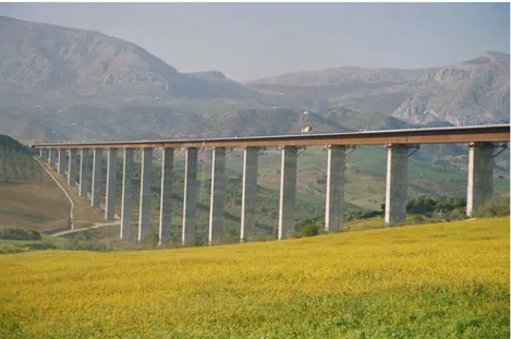
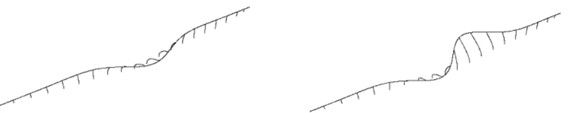
As a representative example we consider the “Arroyo las Piedras” viaduct (Figure 1), with several piers taller than 93 m and a total continuous length of the deck of 1209 m, within the new HSR line Córdoba-Málaga. This deck is a mixed steel-concrete structure with steel girders and concrete slab, with spans of 63,5 m. The design is due to Millanes et al (2007), and the via-duct has been put in operation with the opening of the line to commercial passenger traffic in dec 2007. In Figure 2 the first two modes of vibration are pictured, showing a frequency of 0.29 Hz for the first mode, considerably below the above mentioned requirement for lateral fre-quency.
Figure 2. Modes of vibration 1 (f_1=0.29 Hz) and 2 (f_2=0.37Hz) for viaduct “Arroyo las Piedras”. The lower modes correspond to lateral movement of the deck from bending of the piers.
A similar response in terms of lateral stiffness and vibration modes has been obtained in many other viaducts of similar characteristics in the new HSR lines. However, it must be con-sidered that the modes of deformation involved are global modes of bending due to bending of the piers, with a wavelength of several spans and much longer than one railway car. The ERRI D181 report, Eurocode EN1990-A1 and IAPF requirements refer literally to “the first natural frequency of lateral vibration of a span”, which should be interpreted as the deformation of the deck assuming the supports at the ends of the span rigid.
In order to attain resonance in the vehicles for global lateral deformation modes of long wavelengths it would be necessary for virtually all the vehicles, i.e. the complete train, to oscil-late oscil-laterally in unison, which seems unlikely. More likely the oscil-lateral movements excited in each vehicle will be produced at random phases and cancel each out globally, at least to a certain ex-tent. Finally, we also remark that the main concern in this case refers to the vibration of the ve-hicles and not to the limit states of the bridge which are generally not reached.
The motivation of this work is to assess the lateral deformation of long, laterally flexible via-ducts under traffic loads of HS trains and the associated vibration in the vehicles. The calcula-tions include the main aspects which cause lateral vibration of the vehicles:
1. Lateral displacements in the plane of the track due to deformation of the bridge un-der eccentric vertical traffic loads;
2. Track alignment irregularities;
3. Hunting oscillations from conicity of wheel-rail contact.
The analyses were carried out in two successive calculations. Firstly, the traffic loads were run for different trains at several speeds, and histories of displacements at the track axis were obtained. These histories allowed the generation of virtual paths for the axles of a given bogie. These virtual paths are computed as the lateral deformation experienced at a given axle as a function of the longitudinal coordinate of the same axle with the forward motion of the train. Following, these virtual paths were superposed to track alignment irregularities and hunting os-cillations, and applied to dynamic models which represent the motion of each vehicle. The re-sults obtained are histories of accelerations and displacements at selected locations, as well as histories of loads transmitted by vehicles to the structure.
The methodology outlined above defines the coupling between vehicle in a weak manner, as the ensuing dynamic lateral load histories are not fed back into the structural calculations. It was checked that the deformations of the bridge were small for the lateral loads experienced, and consequently the results could be taken as a valid approximation.
In the remaining of this paper, we first describe the vehicle types and models considered, covering the most representative HSR trains. Following, the actions taken into account are de-fined. A summary of the most representative results is given next. Finally, a set of representative results is shown and analyzed. It is seen that the lateral vibration effects for the cases and as-sumptions considered, although they have a magnitude which should not be neglected, are within allowable bounds.
2 VEHICLE MODELS
A schematic representation of the vehicles is shown in figure 3. The AVE S103 vehicles are
conventional cars with two bogies in each. The AVE S-100 vehicles are articulated, sharing
bo-gies between adjacent cars. Each bogie has two axles, connected to the bogie by the primary suspension; in turn, the bogies are connected to the car body by the secondary suspension. Fi-nally, the UIC freight wagon has only one suspension system connecting the car body directly to the wheelsets.
Figure 3. Vehicle models considered in this study. (a) UIC Freight wagon, (b) Passenger car of AVE S-103 train, (c) Passenger car of AVE S-100 train.
The characteristics of the vehicle models are presented in tables 1 and 2, which were obtained from the references indicated. It must be remarked that some of these parameters are only ap-proximate, namely the values for lateral stiffness, as in some cases exact values for the desired vehicle types could not be obtained. The convention for the axes directions is x for longitudinal,
y vertical and z lateral.
In the case of the articulated AVE S-100 train the model needed to represent not only the cen-tral vehicle but an approximation of the adjacent ones connected to the end bogies as well, with half of the mass of each one. This was essential to model properly the bogies and restrain the yaw rotation. Due to this fact the vehicle model includes primary and secondary longitudinal suspensions also. These data are not included in the other vehicle models because their influ-ence is not relevant.
Table 1. Masses and moments of inertia for the vehicle models (in ton and ton·m2). Data for AVE S-100 from Sang, Noh and Choi (2003), for AVE-S103 and UIC wagon from train manufacturer and ERRI (1996).
__________________________________________________________________________
Vehicle model S-100 S-103 UIC wagon
__________________________________________________________________________ Mass of car body 28.74 33.79 41.0 Mass of bogie 3.02 2.80 - Mass of wheelset 1.58 1.52 2.0 __________________________________________________________________________ Inertia of car body around x axis 34.27 88.5 35 Inertia of car body around y axis 981.34 1570 656 Inertia of car body around z axis 981.34 1540 656 __________________________________________________________________________ Inertia of bogie around x axis 2.03 2.07 - Inertia of bogie around y axis 3.79 1.316 - Inertia of bogie around z axis 3.2 3.052 - __________________________________________________________________________
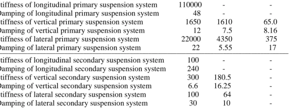
Table 2. Suspension stiffness (kN/m) and damping (kN·s/m) characteristics for the vehicle models. Data for AVE S-100 from Sang, Noh and Choi (2003), for AVE-S103 and UIC wagon from train manufacturer and ERRI (1996, 1998).
______________________________________________________________________________________________
Vehicle model S-100 S-103 UIC wagon
______________________________________________________________________________________________
(a) (b)
Stiffness of longitudinal primary suspension system 110000 - - Damping of longitudinal primary suspension system 48 - - Stiffness of vertical primary suspension system 1650 1610 65.0 Damping of vertical primary suspension system 12 7.5 8.16 Stiffness of lateral primary suspension system 22000 4350 375 Damping of lateral primary suspension system 22 5.55 17 ______________________________________________________________________________________________ Stiffness of longitudinal secondary suspension system 100 - - Damping of longitudinal secondary suspension system 240 - - Stiffness of vertical secondary suspension system 300 180.5 - Damping of vertical secondary suspension system 6.6 16.25 - Stiffness of lateral secondary suspension system 100 64 - Damping of lateral secondary suspension system 30 10 - ______________________________________________________________________________________________
In the models, in terms of boundary conditions, only the reference points at the centre of each wheelset was constrained, in which rotations about the three axes and the longitudinal and verti-cal motions were restrained. Only lateral (z) movement is allowed at these points, to which will be applied given time histories of prescribed motion. The two wheelsets of each bogie are con-sidered to move in parallel with the same time-history, however different input motions are ap-plied to the two bogies. For this reason a single centre of mass was considered for the two wheelsets. As a consequence, the primary suspensions were modeled with the joint properties of the two axles, as depicted in figures 3(b) and 3(c).
These models were developed in the finite element program ABAQUS (HKS (2007). Al-though the main purpose of ABAQUS is deformable bodies it includes also capabilities for mul-tibody systems, allowing the different parts of the vehicles, as the car body, the bogies and the wheelsets, to be taken as rigid bodies. Each body is defined by a number of points, appropriately located in space, one of them being considered as the origin of the reference system. The con-nection between the different bodies/parts is modeled through connector elements, which may represent the suspensions or rigid joints. The suspensions included longitudinal, vertical and lat-eral stiffness and damping properties. As an example figure 4 shows the model of the AVE S-100 train and the respective points of the different parts, marked with yellow spots. The refer-ence points are marked with blue spots.
Figure 4. AVE S-100 finite element vehicle model developed in ABAQUS. Connection points in a bogie of the vehicle and referential axis of the suspensions or connector elements. Reference points for mass and inertia moments are marked in blue.
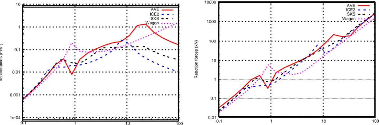
Figure 5. Transfer function for each vehicle model for the lateral accelerations in the centre of mass of the car body (left) and for the lateral reaction forces on the wheelsets of one bogie (right).
3 ACTIONS CONSIDERED
For the dynamic analysis, three different actions responsible for lateral vibration of railway ve-hicles, when crossing a bridge, were considered: 1) lateral displacements in the plane of the track due to deformation of the bridge under eccentric vertical traffic loads, 2) track alignment irregularities and 3) hunting oscillations from conicity of wheel-rail contact.
In order to evaluate the influence of each action in the total lateral dynamic behavior of the vehicle models, three combinations of effects were performed, as follows:
• Combination 1: Bridge lateral displacements only;
• Combination 2: Bridge lateral displacements + track irregularities;
• Combination 3: Bridge lateral displacements + track irregularities + hunting oscilla-tions.
3.1 Bridge lateral displacements
Lateral displacements in railway bridges from traffic loads result from eccentric vertical loads in bridges with double track deck. Two effects from these loads must be considered (figure 6): bending of supporting piers and torsion of the deck.
θ δ1
Support Midspan
δ1 δ2
Figure 6. Representation of lateral displacement of the deck due to bending of the piers δ1 (support sec-tion) and deck torsion δ2 (midspan).
In the following, for considering these displacements the concept termed here virtual path will be used. This is defined as a function
u
z(x
)
representing the displacement of the track (lateral in this case,u
z) at a moving point which follows the train on its motion along the bridge. Note that the virtual path represents the bridge deformation due to train loads, in a structural dynamic model of the bridge, but not considering bridge-vehicle interaction. It may also be represented as a displacement time-history curve, by a simple change of variables. This change represents the equivalence between time and train position,v
=
x
⋅
t
with appropriate choice of zero value of coordinates. Both scales are represented in the virtual paths of figures 7 and 8.1e-04 0.001 0.01 0.1 1 10
0.1 1 10 100
Accelerations (m/s
2)
Frequencies (Hz)
AVE ICE2 SKS Wagon
0.01 0.1 1 10 100 1000 10000
0.1 1 10 100
Reaction forces (kN)
Frequencies (Hz)
Figure 7. Representation of virtual paths due to the passage of the AVE S-100 and AVE S-103 trains: (a) virtual path for an axle of the train S-100 located 200.15 m from the head of the train, at 400 km/h; (b) virtual path for an axle of the S-103 train located 336.06 m from the first axle of the train, at 400 km/h.
0 5 10 15 20 25 30
0 5 10 15 20 25 30 35 1209 m 0 m
Lateral displacement (mm)
Time(s)
Deck lateral displacement without torsion vibration Lateral displacement due to torsion vibration Virtual Path
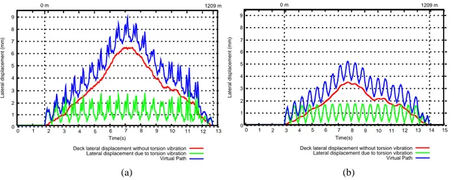
Figure 8. Representation of the virtual path due to the passage of the UIC freight wagon for an axle lo-cated at 425 m from the first axle, at 150 km/h.
A virtual path was computed given for each axle/bogie of the train. In figure 7 the virtual path for the selected axles of the S-100 and S-103 trains are shown, when crossing the “Arroyo las Piedras” viaduct at v = 400 km/h. Each virtual path was obtained at points every 10 cm along the deck. In the figures, the red line represents bending lateral displacements δ1 and the green
line torsional displacements δ2. In blue the total lateral displacement from the two effects is
shown. It may be clearly seen that the bending of piers produces a long wave motion (with wavelength equal to the length of the bridge), whereas the torsional deformations produce a shorter wave motion (with wavelength equal to the span). Furthermore, for some velocities dy-namic amplification from vibration of the bridge is obtained. The bogies or axles have been se-lected to represent worst cases for torsional lateral deformations δ2, which proved to be the
ac-tions with a greater effect on vehicle lateral motion.
3.2 Track alignment irregularities
Railway track irregularities are normally due to wear and tear, clearances, subsidence, inade-quate maintenance, etc. The rail irregularities are assumed to be stationary random and ergodic processes in space, with zero mean values. They are characterized by their respective one sided power spectral density functions,ΦV,A(Ω), in which Ω is the spatial frequency or wave num-ber. In the present study, the power spectral density functions based on measurements per-formed in German railway tracks are adopted, following the empirical formula for alignment ir-regularities proposed by ARGER/F (1980), as used by Claus & Schiehlen (1997):
0 1 2 3 4 5 6 7 8 9
0 1 2 3 4 5 6 7 8 9 10 11 12 13 1209 m 0 m
Lateral displacement (mm)
Time(s)
Deck lateral displacement without torsion vibration Lateral displacement due to torsion vibration Virtual Path
0 1 2 3 4 5 6 7 8 9
0 1 2 3 4 5 6 7 8 9 10 11 12 13 14 15 1209 m 0 m
Lateral displacement (mm)
Time(s)
Deck lateral displacement without torsion vibration Lateral displacement due to torsion vibration Virtual Path
,
)
)(
(
)
(
2 2 2 2 2 ,Ω
+
Ω
Ω
+
Ω
Ω
=
Ω
Φ
c r c AV
A
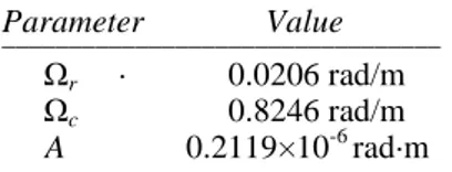
(1)where A, Ωc and Ωr are data which define the actual data, defined in table 3. Sample rail
ir-regularity profiles can be generated numerically using the following harmonic series expansion:
, ) cos( 2 ) ( 1 0
∑
− = + Ω = N n n n n x A xr
ϕ
(2)which represents the spectral density of N discrete frequencies Ωn. The independent random phase angles
ϕ
n are uniformly distributed in the range between 0 and 2π
. Expression (2) is de-fined within an interval of frequencies [Ω0, Ωf], previously established, with an increment setto:
.
0N
f
−
Ω
Ω
=
∆Ω
(3)In turn, An is defined as:
n n
n
S
A
=
(
Ω
)
∆Ω
2
1
π
(4)Table 3. Parameters taken for track alignment irregularities. _________________________________
Parameter Value
_________________________________ Ωr · 0.0206 rad/m Ωc 0.8246 rad/m
A 0.2119×10⁻⁶ rad·m
_________________________________
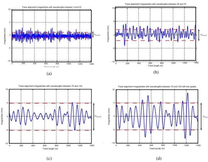
For this study, the value of A was assumed to be equal to 0.2119×10⁻⁶ rad·m which provided sample profiles with similar root mean-square values (standard deviation) to the alert limits pro-posed in CEN (1995b). This code defines these limits in three wavelength ranges for measuring irregularities:
• D1: wavelength of irregularities within the interval 3≤
λ
<25 (m): σlimit =1mm;• D2: wavelength of irregularities within the interval 25≤
λ
<70 (m): σlimit =2mm;• D3: wavelength of irregularities within the interval 70≤
λ
<200 (m): σlimit =5mm.Considering the vehicles at 400 km/h, the previous intervals can be associated to the follow-ing track frequencies intervals (at 150 km/h for the freight wagon the frequencies are corre-spondingly lower): for D1 37≤ f <4.4 (Hz); for D2 4.4≤ f <1.6 (Hz); for D3
9 . 0 6
.
Figure 9. Track alignment irregularities profiles for the different intervals considered. (a) D1, (b) D2, (3) D3 and (4) D3x (with lower track quality). The dashed lines indicate the alert limits for standard devia-tion.
The sample irregularity profiles generated are represented in figure 9. A fourth profile D3x
was generated adopting a lower track quality for the interval D3, with the parameter A three
times bigger than the other cases. The respective alert limits and the obtained values of the stan-dard deviations for irregularities are indicated in table 4.
Table 4. Standard deviations obtained and alert limits for track alignment irregularities. ___________________________________________
Interval σ σlimit
___________________________________________
D1 0.89 mm 1 mm D2 1.4 mm 2 mm D3 1.82 mm 5 mm
D3x 3.45 mm 5 mm
___________________________________________
3.3 Hunting movement
Due to the conicity of the geometry of rail-wheel contact, an oscillatory periodic lateral motion may develop. In the simplest case of one axle and conical wheel profile, this motion is purely harmonic as proven by Klingel in 1883 (see e.g. Esveld (1996)). For ordinary speeds and rail-wheel states this motion is damped out and should not be a significant effect. However, in order to include a worst-case scenario we have included a simple harmonic representation of a hunting movement defined by the Klingel motion:
-10 -5 0 5 10
0 200 400 600 800 1000 1200 1400
Irregularties (mm)
Track length (m)
Track alignment irregularities with wavelengths between 3 and 25
σlimit
-10 -5 0 5 10
0 200 400 600 800 1000 1200 1400
Irregularties (mm)
Track length (m)
Track alignment irregularities with wavelengths between 25 and 70
σlimit
-10 -5 0 5 10
0 200 400 600 800 1000 1200 1400
Irregularties (mm)
Track length (m)
Track alignment irregularities with wavelengths between 70 and 120
σlimit
-10 -5 0 5 10
0 200 400 600 800 1000 1200 1400
Irregularties (mm)
Track length (m)
Track alignment irregularities with wavelengths between 70 and 120 with low quality
σlimit
(a) (b)
) 2 sin( 0
K
L x y
y=
π
, with .2 2
γ
π
r sLk
⋅
= (5)
In this function, y0 is the amplitude of the sinusoidal lateral displacement, Lk the wavelength, r the wheel radius, s the track gauge and
γ
the conicity of the wheel thread (inclination). It is clear that equation (5) introduces an equivalent lateral force into the vehicle model defined by the second derivative in time.A more realistic model should include the creep forces developed at the wheel-rail contact, allowing to model the development or not of such motion depending on the conicity or more generally of the geometry of rail and wheel. However, for the purpose of a worst-case scenario we are considering here this simplified approach. The values adopted for these parameters de-fined are dede-fined in table 5, which have been taken considering the maximum nominal values proposed in the European interoperability criteria for infrastructure ERA (2006).
Table 5. Klingel movement parameter values. __________________________
Parameter Value
__________________________ r 0.46 m s 1.435 m
γ 1:20
Lk 16.055 m
y0 0.003 m
__________________________
4 RESULTS
The calculations were carried out with the actions defined above, by direct integration in time in the ABAQUS finite element program. As previously mentioned, the actions were applied to the models in the centre of the wheelsets of each bogie, with appropriately defined different ac-tions on each bogie or axle of a given vehicle. This consideration is important in order to excite the yaw motion (rotation around vertical y axis) of the car body.
From the analysis of the transfer functions of the vehicle models, presented in section 2, it may be foreseen that the maximum dynamic response will be obtained for actions with higher frequencies of excitation. Thus, it was expected a higher vehicle dynamic response due to the combination of actions with irregularities profiles of short wavelength. This was what effec-tively happened in all the cases except for the UIC freight wagon.
The results for the S-100 train vehicle model are presented in figure 10, in which the lateral accelerations in the centre of gravity of the car body and the lateral reaction forces in the wheel-sets of one bogie are presented. Is possible to see that the accelerations are not high, being be-low the value of 1 m/s2, and the lateral reaction forces on the wheelsets are generally below 100 kN with some isolated peaks of around 200 kN.
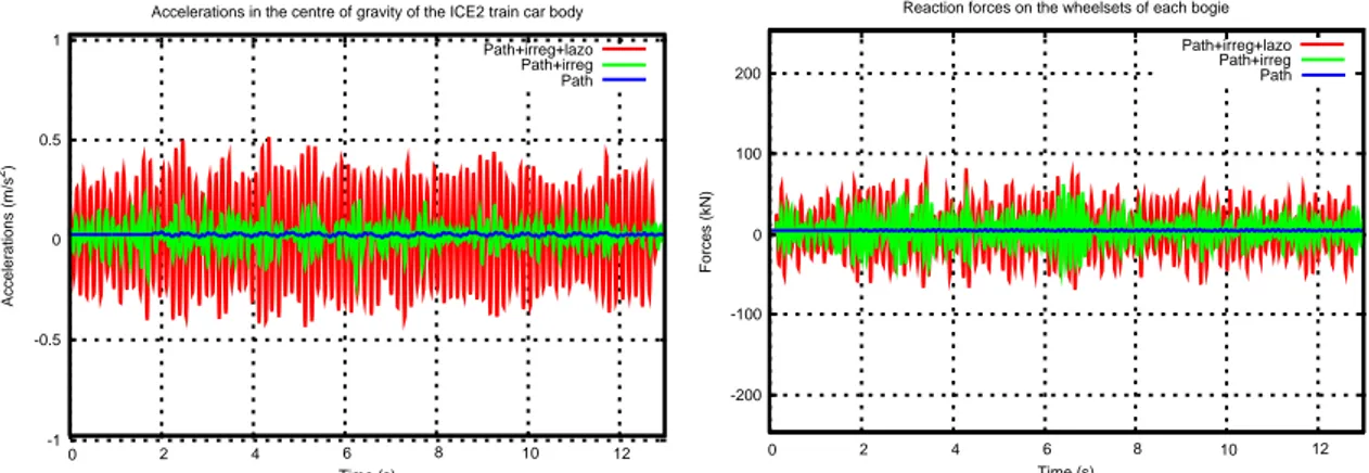
The results for the S-103 vehicle model are shown in figure 11. These are clearly lower than those obtained for the S-100 vehicle model. Accelerations are always below 0.5 m/ s2.
-1 -0.5 0 0.5 1
0 2 4 6 8 10 12
Accelerations (m/s
2)
Time (s)
Accelerations in the centre of gravity of the AVE train car body Path+irreg+Klingel
Path+irreg Path
-200 -100 0 100 200
0 2 4 6 8 10 12
Forces (kN)
Time (s)
Reaction forces on the wheelsets of each bogie Path+irreg+Klingel
Figure 10. Lateral accelerations in the centre of gravity of the car body and lateral reaction forces in the wheelsets of one bogie of the S-100 vehicle model, considering for the combination of action a profile of irregularities with wavelengths within 3 m and 25 m and a speed of 400km/h. In blue the response to only the virtual path (deformation of viaduct), the green curve includes also track irregularities and in red the previous plus hunting motion.
Figure 11. Lateral accelerations in the centre of gravity of the car body and lateral reaction forces in the wheelsets of one bogie of the S-103 vehicle model, considering for the combination of action a profile of irregularities with wavelengths within 3 m and 25 m and a speed of 400 km/h. In blue the response to only the virtual path (deformation of viaduct), the green curve includes also track irregularities and in red the previous plus hunting motion.
For the UIC freight wagon the resonant frequencies of excitation are lower than for the other cases, among other causes due to the maximum speed being 150 km/h. Consequently the maxi-mum response was obtained for alignment wavelengths between 25 and 70 m. The results are presented in figure 12, in which the maximum lateral accelerations are lower than 0.4 m/ s2, and the maximum lateral reaction forces on the wheelsets of one bogie are near 10 kN.
-20 -15 -10 -5 0 5 10 15 20
0 5 10 15 20 25 30
Forces (kN)
Time (s)
Reaction forces on the wheelsets of each bogie Path+irreg+lazo
Path+irreg Path
-0.4 -0.2 0 0.2 0.4
0 5 10 15 20 25 30
Accelerations (m/s
2)
Time (s)
Accelerations in the centre of gravity of the UIC Wagon car body Path+irreg+lazo Path+irreg Path
Figure 12. Lateral accelerations in the centre of gravity of the car body and lateral reaction forces in the wheelsets of one bogie of the UIC freight wagon model, considering for the combination of action a pro-file of irregularities with wavelengths within 25 m and 70 m and a speed of 150 km/h.
5 CONCLUDING REMARKS
The study of the lateral behaviour of railway bridges and vehicles is an important issue on bridges with low lateral stiffness, which has been quantified by ERRI (1996) as those with lat-eral natural frequencies below 1.2 Hz. In principle this limit applies only to the deformation of the deck in one span, and was demonstrated to be a real issue on measurements and models on bridges with open deck sections and supporting trusses, of low lateral bending stiffness for the deck.
Although not included in the above category, modern long viaducts for HSR with continuous decks on tall piers may also exhibit very low lateral stiffness and frequencies. While there is generally no concern for the viaduct itself, there could be undesired effects for the comfort or
-1 -0.5 0 0.5 1
0 2 4 6 8 10 12
Accelerations (m/s
2)
Time (s)
Accelerations in the centre of gravity of the ICE2 train car body Path+irreg+lazo
Path+irreg Path
-200 -100 0 100 200
0 2 4 6 8 10 12
Forces (kN)
Time (s)
Reaction forces on the wheelsets of each bogie Path+irreg+lazo
even the stability of the vehicles. For this purpose one needs to take into account several main factors providing lateral excitation: the lateral deformation of the bridge in response to vertical eccentric loads, the track alignment irregularities and finally lateral motion of vehicles due to conicity of wheel-rail contact.
In this work a simple model has been developed and applied to consider worst-case scenarios in a representative bridge, the “Arroyo de las Piedras” viaduct in Spain. The trains considered are representative of those circulating in the Spanish HSR network, as well as a freight wagon. Three-dimensional dynamic models were developed with finite elements. The results show that there is, at least in this case, no cause for concern. However, for some scenarios the results in terms of lateral motion and forces are not negligible and should be considered in the design.
We are currently working on more realistic models, with full vehicle-bridge interaction, as well as more detailed models of wheel-rail contact. These models should provide a more realis-tic picture of the effects and allow to extract conclusions with greater confidence.
6 REFERENCES
ERRI, 1996. Forces laterals sur les ponts ferroviaires. Rapport finale D181/RP6, European Railway Re-search Institute (ERRI), juin 1996.
ERRI, 1998. Design of railway bridges for speed up to 350 km/h; Dynamic loading effects including
resonance. Technical report D214/RP9, European Railway Research Institute (ERRI).
CEN 2005. EN1990:2002-A1: Eurocode: Basis of Structural Design. Annex A2 Application for bridges. European Committee for Standardization (CEN), Ammendment A1 to EN1990:2002, European Stan-dard, dec 2005.
CEN 2005b. prEN 13848-5, 2005. Railway applications – Track – Track geometry quality – Part 5:
Geo-metric quality assessment. European Committee for Standardization (CEN), Draft European Standard,
may 2005.
MFOM 2007. Instrucción de Acciones en Puentes de ferrocarril (Code for Actions on Railway Bridges), Ministerio de Fomento, Gobierno de España (Ministry of Public Works, Govt. of Spain), 2007. Millanes F, Pascual J & Ortega M, 2007. “Arroyo las Piedras” Viaduct. The first Composite
Steel-Concrete High Speed Railway bridge in Spain. Hormigón y Acero no. 243, pp 5-38.
HKS 2007. ABAQUS/Standard documentation. Hibbit Carlson & Sorensen Inc. Esveld C, 2001. Modern railway track. Second Edition.
Song, Noh & Choi, 2003. A new three-dimensional finite element analysis model of high-speed
train-bridge interactions. Journal of Engineering Structures, Elsevier.
ERA 2006. Interoperability of the transEuropean high speed rail system-“Infrastructure” sub-system. European Railway Agency, EU Directive 96/48/EC, 2006.
ARGER/F, 1980. Arbeitsgemeinschaft Rheine-Freren. Rad/schiene-versuchs- und
demonstrationsfahr-zeug, definitionsphase r/s-vd. Ergebnisbericht der Arbeitsgruppe Lauftechnik, MAN, München.