An embedded cohesive crack model for finite element analysis of quasi-brittle materials

An

embedded

cohesive

crack

model

for

finite

element

analysis

of

quasi-brittle

materials

J.C.

Gálvez

,

J.

Planas

,

J.M.

Sancho

,

E.

Reyes

,

D.A.

Cendón

,

M.J.

Casati

A B S T R A C T

Thispaperpresentsanumericalimplementationofthecohesivecrackmodelfortheanal-ysisofquasibrittlematerialsbasedonthe strongdiscontinuityapproachintheframeworkofthefiniteelementmethod.Asimplecentralforcemodelisusedforthestressversus crackopeningcurve.Theadditionaldegreesoffreedomdefiningthecrackopeningaredeterminedatthecracklevel,thusavoidingthe needforperformingastaticcondensationattheelementlevel.Theneedforatrackingalgorithmisavoidedbyusingaconsistent pro-cedurefortheselectionoftheseparatednodes.Suchamodelisthenimplementedintoacommercialprogrambymeansofauser subroutine,consequentlybeingcontrastedwiththeexperimentalresults.Themodeltakesintoaccounttheanisotropyofthematerial. Numericalsimulationsofwell-knownexperimentsarepresentedtoshowtheabilityoftheproposedmodeltosimulatethefractureof quasibrittlematerialssuchasmortar,con-creteandmasonry.

1. Introduction

Numerical implementation of quasi-brittle cohesive cracking remains an open issue, 30 years after the introduction of the

fictitious crack model by Hillerborg[1]. Traditionally, the numerical methods based on the Finite Element Method (FEM)

were classified into two groups[2]: smeared crack and discrete crack approaches, although some authors include a third

group: the lattice approach[3].

In the smeared crack approach the fracture is represented in a smeared manner: an infinite number of parallel cracks of

infinitely small opening are (theoretically) distributed (smeared) over the finite element[4]. The cracks are usually modelled

on a fixed finite element mesh. Their propagation is simulated by the reduction of the stiffness and strength of the material.

The constitutive laws, defined by stress–strain relations, are non-linear and show astrain softening. This approach was

pio-neered with fixed-crack orthotropic secant models[5–7]and rotating crack models[8–10]. More elaborate models have also

been proposed[11,12].

However, suchstrain softeningintroduces some difficulties in the analysis. The system of equations may become ill-posed

[13–15], localisation instabilities and spurious mesh sensitivity of finite element calculations may appear[4]. These

the non-local continuum models[19,20], the gradient models[21], and the micropolar continuum[22]. These procedures are suited to specific problems, but none gives a general solution to the problem.

The discrete approach is preferred when there is one crack, or a finite number of cracks, in the structure. The cohesive

crack model, developed by Hillerborg and co-authors[1]for mode I fracture of concrete, was shown to be efficient to model

the fracture process of quasi-brittle materials. It has been extended to mixed mode fracture (modes I and II) and incorporated

into finite element programs[23–28]and into boundary element codes[29]. One of the difficulties associated with these

programs is that they require the remeshing and/or refinement of the finite element mesh when the crack grows, and some of them also require an input of material properties that are difficult to evaluate.

In recent years, a new methodology based on the so-calledstrong discontinuity approach(SDA) has been proposed[30,31].

The SDA complements the classical approaches, the smeared crack and the discrete crack, and has been successful in the analysis of the fracture of quasibrittle materials. In contrast to the smeared crack model, in the SDA the fracture zone is rep-resented as a discontinuous displacement surface. Different from the discrete crack approach, in the SDA the crack geometry

Nomenclature

a finite element node index

A finite element area

ba(x) shape function gradient for nodea

E elastic moduli tensor

f(w) classical softening function for mode I

ft tensile strength

ft1 tensile strength in the material axis1(bed joints direction)

ft2 tensile strength in the material axis2(head joints direction)

GF specific fracture energy

h triangular element height

H(x) Heaviside jump function

L crack length in the finite element

n unit normal vector

Na(x) traditional shape function for nodea

t traction vector

ua nodal displacement

w crack opening

w crack displacement vector

~

w equivalent crack opening

a

angle between the material axis1(bed joints direction) and theOXaxis

b angle between the first principal stress direction and theOXaxis

c

angle between the crack direction and the material axis1(bed joints direction)

e

c _{continuous part of the strain tensor}

e

a _{apparent part of the strain tensor}

r

stress vector, with components (

r

x,

r

y,

s

xy)

h angle between first principal stress direction and the material axis1(bed joints direction)

r

I first principal stress

r

c normal stress to the arbitrary direction (which forms an angle

c

with the material axis1)

1 direction of the bed joints of masonry

2 direction of the head joints of masonry

I first principal stress direction

II second principal stress direction

Abbreviations

CMOD crack mouth opening displacement

CMSD crack mouth sliding displacement

EAS enhanced assumed strain method

FE finite element

FEM finite element method

SDA strong discontinuity approach

is not restricted to interelement lines, as the displacement jumps are embedded in the corresponding finite element

dis-placement field. A comparative review of the various approaches to the embedded crack concept is presented by Jirásek[32].

Embedding discontinuous displacements in the element formulation is not the only way to implement the SDA in the

finite element method. Recently the so-calledextended finite element method, based on nodal enrichment and the partition

of the unity concept, has opened a very fruitful way to the modelling of fracture. However, extended finite elements require a greater implementation effort compared with elements with embedded discontinuities. The advantages and disadvantages

of both strategies can be found in[33–36].

This work presents a procedure, based on the SDA, which reproduces the fracture process of the quasi-brittle materials under mixed loading using the cohesive crack approach. The paper tries to show how, by means of simple considerations, using finite elements with embedded cohesive crack is one of the more efficient of options to model the mixed mode fracture of concrete.

The SDA provides a consistent framework to transform a weak discontinuity, in which the displacement is continuous but

the strain is discontinuous at the boundaries of a band of a certain widthh, into a strong discontinuity in which the

displace-ment is discontinuous at a surface. Thus, the strong discontinuity (displacedisplace-ment jump) is obtained as the limit of a weak

discontinuity band when the bandwidthhtends to zero. In this way the discrete constitutive model for the discontinuity

naturally arises, being induced by the continuum model. This is an elegant and sound standpoint for the study of shear bands in soils and metals. However, in the fracture of quasibrittle materials, it is simpler and more effective to use a discrete con-stitutive model that relates the tractions and displacement jumps at the discontinuity line. This approach is used in the pres-ent work.

A consistent derivation of finite element with embedded discontinuities can be performed in the frame of the enhanced

assumed strain method (EAS) proposed by Simo and Rifai[37]. The strain induced for the displacement jumps are then

tack-led as additional incompatible modes. A problem of this approach is that, as the additional modes are determined at the ele-ment level, the progress of the crack may be locked because of kinematical incompatibility between the cracks in neighbouring elements.

One solution to avoid this problem is to use an algorithm to re-establish the geometric continuity of the crack line across

the elements, a procedure known as cracktracking[38]. Most practical implementations use tracking to avoid crack locking.

Moreover, some implementations further require establishing exclusion zones defined to avoid the formation of new cracks in the neighbourhood of existing cracks. This kind of algorithms present some degree of inconvenience in the implementa-tion of the embedded crack elements in standard finite element programs, and development of a method that circumvents the need of the crack path enforcement is therefore of greater interest.

The proposed model has been incorporated into commercial multipurpose finite element programs by means of a user subroutine, and contrasted with the experimental sets of mixed mode fracture of quasibrittle materials from the literature. The model only requires standard properties of the material, measured by standardised methods.

2. The cohesive crack model

2.1. Overview of the cohesive crack model for isotropic materials

Previous works showed that for most experiments described in the literature, cohesive crack growth takes place under

predominantly local mode I, which implies that the overall behaviour is dominated by mode I parameters[27,39]. Therefore,

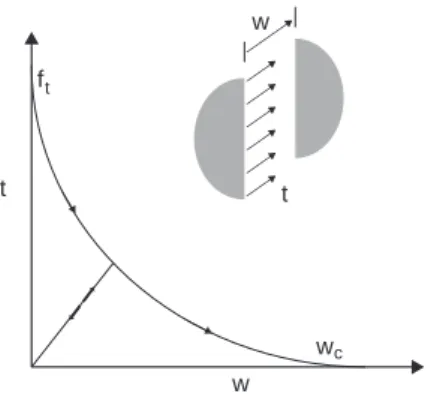
in this work, a simple generalisation of the cohesive crack to mixed mode is used which assumes that the traction vectort

transmitted across the crack faces is parallel to the crack displacement vectorw(central forces model). For monotonic

load-ing in which the magnitude of the crack openload-ing vector |w| is never decreasing, the relationship reads:

w wc

f_t

t

w

t

t¼fðjwjÞw

jwj ð1Þ

wheref(|w|) is the classical softening function for pure opening mode (Fig. 1). To cope with the possibility of unloading, it is

further assumed that the cohesive crack unloads to the origin (Fig. 1) and Eq.(1)is rewritten as:

t¼fðj_~w~jÞ

w w with w~¼maxðjwjÞ ð2Þ

where isw~ an equivalent crack opening defined as the historical maximum of the magnitude of the crack displacement

vector.

2.2. Cohesive crack model for anisotropic materials

On isotropic quasibrittle materials the cohesive crack initiates at the point where the maximum principal stress

r

Ifirst

reaches the tensile strengthft, and the crack grows in a normal direction to that of the maximum principal stress. Then, the

crack grows predominantly under local mode I. This approach is not valid for anisotropic cohesive materials, such as brick masonry, where the cracking initiation and growth cannot be exclusively expressed in terms of principal stresses, and a fail-ure criterion is also needed. There is significant experimental evidence about the dependence of the crack path orientation in

brick masonry with the direction of the bed joints[40].

The Rankine criterion has been successfully used as a cracking criterion for quasi-brittle materials. In this work a gener-alised the Rankine criterion has been adopted. This criterion balances accuracy and simplicity, especially from the point of view of the experimental determination of the mechanical parameters of the brick masonry, which is the anisotropic quasi-brittle material adopted in this work for the model validation.

Fig. 2shows the sketch of an anisotropic material (a panel of brickwork masonry). Axis1and axis2show the direction of

the material axes (bed and head joints of the masonry), respectively.OXandOYare the axes of reference in a numerical

sim-ulation.IandIIshow the principal stress directions.

a

is the angle betweenOXaxis and1direction.bis the angle betweenOX

axis andIdirection.hangle measures the rotation between principal stress axis with respect to the principal material axes,

and is the addition of the angles

a

andb.

The direction at which the crack initiates, given by the angle

c

relative to1direction, is unknown. Such a direction is one

in which the tensile stress reaches the tensile strength. It is worth noting that whereas in an isotropic material the direction when the crack initiates is given by the maximum principal stress, in anisotropic material there could be another direction in which the tensile stress reaches the strength of the material.

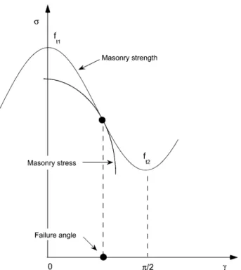
To complete the generalised Rankine criterion it would be of interest to measure the tensile strength of the masonry in different directions, which is quite difficult to carry out in practice. For the sake of simplicity, in this work the material is

characterised in two representative directions: for example, in their principal directions, and then a function of angle

c

is

adopted to evaluate the strength in the intermediate directions. To avoid possible convergence problems caused by kink

points, a sinusoidal curve has been adopted (seeFig. 3). So, the tensile strength is expressed as:

ftð

c

Þ ¼ ft1þft2

2 þ

ft1ft2

2 cosð2ð

c

ÞÞ ð3Þ

Due to the symmetry of the brickwork masonry, this function is symmetrical concerning the axisft(

c

), and has a period of

p

.

In accordance with Eq.(2), the tensile strengthft(

c

) evolves with the softening parameterw~, from intact tensile strength

until zero, when the masonry is completely broken. The difference with isotropic material is the dependence of the tensile

strength with angle

c

.

The stress state at any point of the masonry, in a 2-D analysis, is given by the stress tensor

r

. The normal stress to an

arbitrary direction, which forms an angle

c

with the axis1(direction of the bed joints), may be expressed as:

r

c¼ ð

r

~ucÞn¼

r

xþ

r

y

2 þ

r

x

r

y

2 cosð2ð

c

þ

a

ÞÞ

s

xysenð2ð

c

þ

a

ÞÞ ð4Þ

The crack initiates (or grows) in this direction (angle

c

with bed joints) if

r

creaches the actual tensile strength in the normal direction to this one, expressed as:

r

c¼ftð

c

Þ ð5Þ

Eq.(5)is a necessary condition though inadequate, given that these two curves,

r

candft(

c

), must intersect at one point.

Consequently, as they also have to be tangent at this point, the following additional condition is imposed (seeFig. 3):

d

r

c d

c

¼

dftð

c

Þ

d

c

ð6Þ

3. Finite element modelling

This section provides the modelling to describe the masonry cracking in 2D. For this purpose the crack is numerically implemented as a discontinuity embedded in a classical FE. The modelling is mainly based on the authors’ proposal for

con-crete[41–43]and masonry[44].

3.1. Overview of the FE formulation

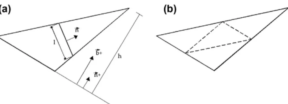
Let be an arbitrary classical finite element defined by a node layout as shown inFig. 4a. Assume that a straight crack is

embedded in it. Take one of the faces of the crack as the reference and its normalnpointing towards the other face as the

positive normal. Letwbe the displacement jump across the crack of the opposite side of the crack with respect to the

reference side (seeFig. 4b). The crack splits the element in two sub-domainsA+_{andA. Following the SDA (e.g.,[45]), the} approximated displacement field within the element can be written as:

uðxÞ ¼X

a2A

NaðxÞuaþ ½HðxÞ NþðxÞw ð7Þ

whereais the element node index,Na(x) the traditional shape function for nodea,uathe corresponding nodal displacement,

H(x) the Heaviside jump function across the crack plane [i.e.,H(x) = 0 forx2A_{,H(x) = 1 forx2A}+_{], andN}þ_{ðxÞ ¼}P

a2AþNaðxÞ.

The strain tensor is obtained from the displacement field as a continuous partecplus a Dirac’sdfunction on the crack line.

The continuous part, which determines the stress field on the element on both sides of the crack, is given by

e

c_{ðxÞ ¼}

_e

a_{ðxÞ ½b}þ

ðxÞ wS ð8Þ

whereeaandb+_{are given by}

e

a_{ðxÞ ¼}X

a2A

½baðxÞ uaS ð9Þ

bþðxÞ ¼X

a2Aþ

baðxÞ ð10Þ

withba(x) = gradNa(x) and superscriptsindicating a symmetric part of a tensor. Obviously,eais theapparentstrain tensor of

the element computed from the nodal displacements.

3.2. Crack tractions

Along the cohesive crack line, the jump vectorwand the traction vectortare to be related by Eq.(2)and the

consider-ations expressed by Eq.(5). For the exact solution, the traction vector is computed locally ast=

r

n. For the finite element,

however, approximate tractions and crack jump vectors must be addressed, and there is not a single way to determine the relationship between the approximate stress field and the tractions. To simplify the reasoning, the traction field is estimated

along the crack line by a constant traction_{t. The determination oftis approximate, and can be carried out in two different}

ways: (1) as an average along the crack line of the local traction vector

r

n, or (2) by forcing the global equilibrium of either

A+_{orA(which is equivalent, in this case, to using the principle of virtual work). The corresponding equations read:}

_t¼1 L Z

L

r

ndl ð11Þ

_t¼1 L Z

A

r

bþdA ð12Þ

in which the stress tensor is that corresponding to the classical finite element approximation based on the continuous strain

in Eq.(8). In general, the two equations do not coincide, as shown below for the constant strain triangles with an embedded

crack.

3.3. The constant strain triangular finite element

In this work, the simplest finite element has been selected. If a constant strain triangle with a strong discontinuity line

(crack) is considered, such as that shown inFig. 5a, and the positive normal pointing towards the solitary node is selected,

then it can be shown that

bþ¼1

hn

þ _ð13Þ

wherehis the height of the triangle over the side opposite to the solitary node andn+_{the unit normal to that side. With this,}

and the fact that the stresses are uniform, Eqs.(11) and (12)are reduced to

_t¼

_r

_{n for local equilibrium ð14Þ}

_t¼A hL

r

n

þ _{for global equilibrium ð15Þ}

whereAis the area of the element andLthe length of the crack. This shows that for local and global equilibria to hold, it is

required thatn+_{=nandhL = A. As a result of this, the following two conditions are imposed: (1) the discontinuity (crack) line}

being parallel to one of the sides of the triangle, and (2) the discontinuity line being located at mid-height. Thus, the potential

crack lines satisfying both local and global equilibrium are those indicated by dashed lines inFig. 5b.

In our approach the local equilibrium Eq.(14)is used in conjunction with the strain approximant (8). This leads to a

non-symmetric formulation (SKON, according to Jirásek’s nomenclature[32]). If Eq.(15)is imposed, then a symmetric

formula-tion is obtained (Jirásek’s KOS formulaformula-tions[32]). Note, however, that both formulations tend to coincide when the crack

runs parallel to one side of the element and at mid height (notthrough the centroid).

4. Numerical implementation

To simplify the computations, the bulk behaviour (material outside the crack) is assumed to be linear-elastic and

aniso-tropic, although this approximation can be relaxed if necessary (e.g.[46]). The crack displacement vectorwis handled as two

internal degrees of freedom which are solved at the level of the crack within the finite element (assumed to be a constant strain triangle).

4.1. Basic equations

One of the main tasks of the implementation is to compute the stress tensor in the element, which follows an algorithm

similar to plasticity, since the stress tensor is given, from Eq.(8)and the hypothesis of elastic bulk material behaviour, as

r

¼E:½

e

a

ðbþwÞS ð16Þ

whereEis the tensor of elastic moduli. Before computing the result of the stress, the crack displacement must be solved. The

corresponding equation is obtained by substituting the foregoing expression for the stress into Eq.(14)and the result into

the cohesive crack Eq.(2). The resulting condition is

fð_w~_Þ ~

w w¼ ½E:

e

a _n

½E:ðbþwÞSn ð17Þ

which can be rewritten as

fð_w~_Þ ~

w w¼ ½E:

e

a _{n ½nEb}þ

w ð18Þ

or else

fðw~Þ

~

w 1þnEb

þ

w¼ ½E:

e

a _{n ð19Þ}

where1is the second-order unit tensor. This equation is solved forwusing Newton Raphson’s method given the nodal

dis-placements (and soea) once the crack is formed and thusnandb+_{are also obtained. It is worth noting thatEandfðw~Þ}

de-pends on the direction (angle

c

).

One of the key points in the proposed method is how the crack is introduced in the element, i.e., hownandb+_are

determined.

4.2. Crack initiation

Initially,w =0 in the element, andnandb+_{are undefined. Thus, the element loads elastically and}

_r

_=E:ea_{until the tensile}

stress reaches tensile strength in a particular direction, as shown in Section 2.2. Then a crack is introduced perpendicular to

the direction of the tensile stress that reached the tensile strength, andn,given that it is the unit normal vector to the crack,

is computed as a unit eigenvector of

r

.

Next, the solitary node and the vectorb+_{are determined by requiring the angle betweennandb}+_{to be the smallest}

pos-sible (seeFig. 5). This is based on the fact that the tensornEb+_{, and therefore the tangent stiffness matrix, is well}

automatically avoided. For a constant strain triangle finite element, and given the direction of cracking, there are only three different modes of separating the nodes in two subelements. This is algorithmically achieved by looping over the three

pos-sible vectorsb+_{and looking for the one satisfying}

jbþnj

jbþj ¼max ð20Þ

4.3. Crack adaptation

The foregoing procedure is carried out at the element level, and is strictly local: no crack continuity is enforced or crack exclusion zone defined. This leads in many circumstances to locking after a certain crack growth. Such locking seems to be

due to a bad prediction of the cracking direction in the element ahead of the pre-existing crack, as sketched inFig. 6. To

over-come this problem without introducing global algorithms (crack tracking and exclusion zones), a certain amount of crack adaptability within each element is merely introduced. The rationale behind the method is that the estimation of the prin-cipal directions in a triangular element is especially bad at crack initiation due to the high stress gradients in the crack tip zone where the new cracked element is usually located; after the crack grows further, the estimation of the principal stress directions ordinarily improves substantially. Therefore, the crack is allowed to adapt itself to the later variations in the

prin-cipal stress directionwhile its opening is small. This crack adaptation is implemented very easily by stating that while the

equivalent crack opening at any particular element is less than a threshold valueweth, the crack direction is recomputed

at each step as if the crack were freshly created. Afterwe >weth, no further adaptation is allowed and the crack direction

be-comes fixed.

Threshold values must be related to the softening properties of the material, and values of the order of 0.10.2GF/ftare

usually satisfactory. Here,GFis the fracture energy andftthe tensile strength. Until an in-depth parametric study is carried

out, this is an orientative value to be taken as a starting point for analysis, since the dependence on the threshold may be dependent on the geometry and material properties. This simple expedient has proved to be extremely effective as shown in the examples presented next, and bears some resemblance to other approaches used to avoid crack locking.

5. Numerical analysis of the fracture tests

5.1. Numerical tools

The described model has been introduced in the commercial finite element code ABAQUSÓ[47]by means of a user

mate-rial subroutine (UMAT). An auxiliary external file containing the nodal coordinates and mesh connectivity is also used. This file would not be needed if the model were implemented as a user element in a UEL subroutine. Nevertheless, the use of a

UMAT subroutine avoids the formulation of the whole finite element (v. gr.shape functions) since the program automatically

does this. The model has also been implemented into the FEAP[48]code with a user subroutine. The independence of the

finite element mesh (structured/unstructured and coarse/fine) was previously studied for the isotropic model[42].

5.2. Comparison with the experiments by Arrea and Ingraffea

The experimental results published by Arrea and Ingraffea[49]are traditionally used to verify normal/shear cracking of

concrete models. This pioneering work on mixed mode fracture of concrete serves as a benchmark for validation of numer-ical and analytnumer-ical fracture models.

The only material properties measured in the tests by Arrea and Ingraffea [49]are the compressive strength,fc, the

Young’s modulus,E, and the Poisson’s ratio,

m

. There are no data about the tensile strength,ft, or the specific energy fracture,

GF, both essential to defining the softening curve. Saleh and Aliabadi[29]validated their numerical model by takingft= 2.8

-MPa andGF= 100 N/m. Xie and Gerstle[24]for the same set of tests took:ft= 4.0 MPa andGF= 150 N/m; obviously, the

con-crete fracture parameters are quite different. A relatively small number of beams were tested in each series. Mortar tests

(seriesA): two beams, with one test being valid. Concrete tests: seriesB, with all three beams being valid; and seriesC, in

this case three beams, with only two being valid. A wide experimental scatter band is shown in these tests[49]for the crack

paths and the load-CMSD curves. These drawbacks suggest that a complementary set of experimental data is needed for an

objective validation of the mixed mode cracking models. In this work the seriesBis adopted for comparison.

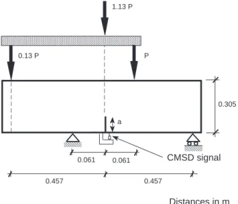
Fig. 7shows the geometry, forces and boundary conditions of the tests Arrea and Ingraffea[49]. The thickness of the

beams was 152 mm.Table 1shows the material properties considered in the simulation; the values of the tensile strength,

ft, and the specific fracture energy,GF, were estimated from the material properties in Arrea and Ingraffea[49]and the

rec-ommendations of the Model Code[50].

Fig. 8shows a deformed mesh, with finite elements with the embedded crack, used to simulate the mixed mode fracture

of theBtest series of Arrea and Ingraffea[49].

5.3. Comparison with the experiments by Gálvez et al.

As stated above, further experiments on mixed mode fracture with notched beams are required for an objective validation

of the numerical procedure. Experimental data on mixed mode fracture of concrete were published by Gálvez et al.[51]. Two

sets of the testing procedure were developed under proportional and non-proportional loading for two different families of

crack paths.Fig. 10shows the geometry, forces and boundary conditions of the tests. The thickness of the beams was 50 mm.

Table 1shows the material properties experimentally measured and used in the numerical simulation. The tensile strength, Fig. 6.Sketch of the crack locking: the prediction of cracking direction in the shaded element is wrong.

a P

0.305

0.061

CMSD signal

0.13 P

1.13 P

0.061

0.457 0.457

Distances in m

Fig. 7.Geometry, forces and boundary conditions of the tests of Arrea and Ingraffea[49].

ft, and the specific energy fracture,GF, were measured with independent tests, according to ASTM C 496[52]standard and

RILEM 50 FMC[53]recommendation, respectively.

Fig. 11shows a deformed mesh, with finite elements with the embedded crack, used to simulate the mixed mode fracture

of thetype 2tests of Gálvez et al.[51].

Fig. 12shows the experimental envelope and the numerical prediction of the loadPversus CMOD curves of teststype 1. Fig. 13shows the experimental envelope and the numerical prediction of the loadPversus displacement curves of teststype

2. In both figures the peak load, the initial part of the curve and descending branch properly fit in the scatter band. The long

tail of the numerical curve presents neither problems of numerical convergence nor occurrence of locking.

5.4. Comparison with the experiments by Schlangen and van Mier

Fig. 14shows the geometry, forces and boundary conditions of the tests by Schlangen and van Mier[54,55]. The thickness of the beams was 100 mm. The material properties adopted in the simulation were based on the values used by other

authors[56].Table 1shows these values.Fig. 15shows the load versus CMSD curve compared with the quantities measured

by Schlangen[54,55]. No locking occurs, and the peak load and initial part of the curve are correctly predicted by the model.

The prediction of the tail could be improved by selecting a softening curve with a steeper initial descent and a stronger tail (a bilinear type of softening).

5.5. Comparison with the experiments by Shi et al.

The other test analysed is a double edge notched specimen subjected to direct tension as shown inFig. 16a. A series of

tests on this type of beam were reported by Shi et al.[57]. Various authors have used this beam as a benchmark for numerical

Table 1

Mechanical properties of the concrete.

Concrete GF(N/m) ft(MPa) E(GPa) m

Arrea and Ingraffea[49] 105 3.5 24.8 0.18

Gálvez et al.[51] 69 3.0 38 0.2

Schlangen[54,55] 100 2.8 35 0.15

Shi et al.[57] 50 3.0 31 0.2

Fig. 8.Deformed finite element mesh of the tests of Arrea and Ingraffea[49].

models.Fig. 16b shows a deformed mesh, with finite elements with the embedded crack, used to simulate the fracture of the

specimens.Table 1shows the material properties adopted in the numerical simulation[56].

Fig. 17shows the experimental results and the numerical prediction of the loadPversus displacement curves. The peak load, the initial part of the curve and descending branch properly fit with the experimental curve. The long tail of the numer-ical curve does not seem to show any problem of numernumer-ical convergence or evidence of locking.

5.6. Comparison with the experiments by Reyes et al.

To check the model with an anisotropic material, the experimental data published by Reyes et al.[58,59]were

numeri-cally simulated. This is a series of mixed mode fracture performed on small masonry panels (a scale factor of1₌

4) under TPB

K= (Type 2 tests) K=0 (Type 1 tests)

D/2 P

B

150

37.5 300

75 225

37.5

CMOD controlling signal 150

(Distances in mm)

∞

Fig. 10.Geometry, forces and boundary conditions of the tests of Gálvez et al.[51].

Fig. 11.Deformed finite element mesh of the teststype 2of Gálvez et al.[51].

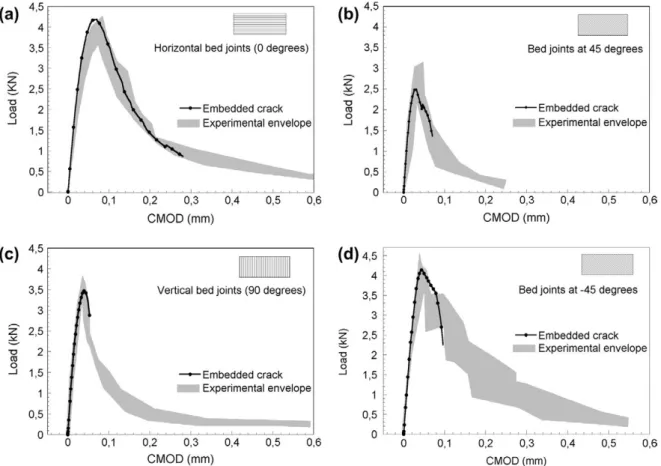
configuration with non-symmetric loading.Fig. 18shows the geometry, forces and boundary conditions of the tests. Twelve

masonry panels of four orientations of the joints (0°, ±45°and 90°), were tested.Table 2shows the mechanical properties of

the masonry. The tensile strength, ft, and the specific energy fracture,GF, were measured with independent tests on

Fig. 13.Experimental envelope and numerical prediction of the teststype 2of Gálvez et al.[51]: LoadP–displacement of the point where the loadPis applied curves.

100 20

P/11 10 P/11

20

180 180

Distances in mm

20

Fig. 14.Geometry, forces and boundary conditions of the tests of Schlangen and van Mier[54,55].

specimens with three orientations of the joints (0°, 45°and 90°). Recommendations of RILEM 50 FMC[52]were adapted to

this material. See[46,58]for details.

Fig. 19shows the experimental and the numerical prediction of the crack paths for the specimens with the four orienta-tions of the bed joints. The numerical prediction is a sufficiently accurate approximation of the crack path. In this sense, it is noticeable that masonry exhibits a wider experimental scatter than other quasi-brittle materials such as mortar and concrete.

60

60 60

15

Distances in mm

(a)

(b)

Figs. 20 and 21compare the envelope of the experimental records load versus CMOD and load versus displacement of the application point of the load for specimens and different orientations of bed joints, with the numerical prediction.

6. Final remarks and conclusions

A numerical model, based on the embedded strong discontinuity approach, is proposed to model the mixed mode fracture

of quasi-brittle isotropic and anisotropic materials. As in previous works[41–44], based on this approach, the deformation is

localised on a line using the concept of the cohesive crack, and the discrete constitutive relation for mixed mode fracture is a

cohesive crack with a central-force model. The model avoids crack tracking[45,60]or exclusion zones for crack growing.

A triangular constant strain finite element is formulated and implemented in the commercial standard programmes

ABA-QUSÓ[47]and FEAP[48]. The choice of the solitary node is made in a way that leads to the automatic propagation of the

Fig. 17.Experimental envelope and numerical prediction of the tests Shi et al.[57]: Load–displacement curves.

Fig. 18.Testing arrangement, geometry, dimensions, boundary conditions and instrumentation of the tests of Reyes et al.[58,59].

Table 2

Mechanical properties of brick masonry under mode I fracture[58,59].

Orientation GF(N/m) ft(N/mm2) E(kN/mm2)

Horizontal 75 5.8 28

45° 54 4.1 22

Fig. 19.Mean experimental (from three specimens) and numerical prediction of the crack path of the specimens of the tests of Reyes et al.[58,59]with the bed joints at: (a) 0°, (b) 45°, (c) 90°, and (d)45°.

crack without tracking algorithm or exclusion zones. The stress locking effects are solved by allowing the embedded crack in the finite element to adapt itself to the stress field while the crack opening does not exceed a small threshold value. This solution may bias the crack orientation, but in comparison with other models, which set a global tracking of the crack, this approach performs it locally. In the authors’ opinion it is an advantage despite its limitations, and accurately predicts the experimental results. A generalised Rankine criterion is adopted with the aim of taking into account the anisotropy of the quasi-brittle materials.

Several series of fracture tests on isotropic and anisotropic material specimens were adopted for checking the model. The numerical model correctly predicts the experimental results.

The proposed model procedure reaches a balance between accuracy and simplicity, and provides a helpful tool in predict-ing the fracture of large masonry structural elements when a spredict-ingle macro-crack, or finite number of them, is the main failure mechanism. The presented model does not include distributed cracking or damage in the structure and applies in the case of

a macro-crack occurring, though such an approximation can be relaxed if necessary[46].

The numerical simulations show that the foregoing combination of simple ingredients leads to a method in which the cohesive crack automatically propagates without the need for a tracking algorithm or exclusion zones. Hence, the embedded cohesive crack approach emerges as an effective and simpler alternative to other more sophisticated methods for the sim-ulation of concrete damage and fracture.

Acknowledgements

The authors gratefully acknowledge the financial support for the research provided by the Spanish Ministerio de Ciencia e Innovación under Grants DPI2011-24876, IPT-42000-2010-31 and BIA2010-18864.

References

[1] Hillerborg A, Modéer M, Petersson P. Analysis of crack formation and crack growth in concrete by means of fracture mechanics and finite elements. Cem Concr Res 1976;6:773–82.

[3] Schlangen E, Van Mier JG. Mixed-mode fracture propagation: a combined numerical and experimental study. In: Rossmanith HP, editor. Fracture and damage of concrete and rock. E&FN Spon; 1993. p. 166–75.

[4] Bazant ZP, Planas J. Fracture and size effect in concrete and other quasibrittle materials. New York: CRC Press; 1998.

[5] Rashid Y. Analysis of prestressed concrete pressure vessels. In: Balkema, editor. Nuclear engineering and design. Rotterdam; 1968. p. 265–86. [6] Cervenka V. Inelastic finite element analysis of reinforced concrete panels under in-plane loads. Ph.D. thesis. University of Colorado; 1970. [7] Suidan M, Schnobrich W. Finite element analysis of reinforced concrete. J Struc Div ASCE 1973;99:2109–22.

[8] Cope R, Rao P, Clark L, Norris P. Modelling of reinforced concrete behaviour for finite element analysis of bridge slabs. In: Taylor C, editor. Numerical methods for non-linear problems. Pineridge Press; 1980. p. 457–70.

[9] Gupta A, Akbar H. Cracking in reinforced concrete analysis. J Struct Engng ASCE 1984;110:1735–46.

[10] Willam K, Pramono E, Stur S. Fundamental issues of smeared crack models. In: Shah, Swartz, editors. Proc SEM-RILEM int conf on fracture of concrete and rock. SEM; 1987. p. 192–207.

[11] de Borst R, Nauta P. Non-orthogonal cracks in a smeared finite element model. Engng Comput 1985;2:35–46. [12] Rots J. Computational modelling of concrete fracture. Ph.D. thesis. Delft University; 1988.

[13] Hill R. Bifurcation and uniquess in non-linear mechanics continua. In: Problems in continuum mechanics. SIAM; 1961. p. 155–64. [14] Mandel J. Conditions de stabilité et postulat de Drucker. In: Rheology and soil mechanics, IUTAM symp. Springer Verlag; 1964. p. 56–68. [15] Carol I, Prat P, López M. Normal/shear cracking model: application to discrete crack analysis. J Engng Mech ASCE 1997;123:765–73. [16] Bazant ZP, Oh B. Crack band theory for fracture of concrete. Mater Struct 1983;16:155–77.

[17] Willam K. Experimental and computational aspects of concrete fracture. In: Damjanic F, et al., editors. Computer aided analysis and design of concrete structures. Pineridge Press; 1984. p. 33–70.

[18] Rots J, Nauta P, Kursters G, Blaauwendraad J. Smeared crack approach and fracture localization in concrete. HERON 1985;30:1–48. [19] Bazant ZP, Pijaudier-Cabot G. Nonlocal continuum damage, localization, stability and convergence. J Appl Mech 1988;55:287–93. [20] Bazant ZP, Ozbolt J. Nonlocal microplane for fracture, damage and size effect in structures. J Engng Mech ASCE 1990;116:2485–504. [21] de Borst R, Mühlhaus M. Gradient dependent plasticity: formulation and algorithmic aspects. Int J Numer Meth Engng 1992;35:521–39. [22] Steinmann P, Willam K. Finite element analysis of elastoplastic discontinuities. J Struct Div ASCE 1994;120:2428–42.

[23] Cervenka J. Discrete crack modelling in concrete structures. Ph.D. thesis. University of Colorado; 1994. [24] Xie M, Gerstle W. Energy-based cohesive crack propagation modelling. J Engng Mech 1995;121:1349–58.

[25] Reich R, Plizzari G, Cervenka J, Saouma V. Implementation and validation of a nonlinear fracture model in 2D/3D finite element code. In: Wittmann, editor. Numerical models in fracture mechanics. Balkema; 1997. p. 265–87.

[26] Valente S. On the cohesive crack model in mixed-mode conditions. In: Fracture of brittle disordered materials, concrete, rock and ceramics. E&FN Spon; 1995. p. 66–80.

[27] Cendón DA, Gálvez JC, Elices M, Planas J. Modelling the fracture of concrete under mixed loading. Int J Fract 2000;103:293–310.

[28] Gálvez JC, Cervenka J, Cendón DA, Saouma V. A discrete crack approach to normal/shear cracking of concrete. Cem Concr Res 2002;32: 1567–85.

[29] Saleh A, Aliabadi M. Crack growth analysis in concrete using boundary element method. Engng Fract Mech 1995;51:533–45.

[30] Simo J, Oliver J, Armero F. An analysis of strong discontinuities induced by strain softening in rate-independent inelastic solids. Comput Mech 1993;12:277–96.

[31] Simo J, Oliver J. A new approach to the analysis and simulation of strong discontinuities. In: Fracture and damage in quasi-brittle structures. E&FN Spon; 1994. p. 25–39.

[32] Jirásek M. Comparative study on finite elements with embedded cracks. Comput Methods Appl Mech Engng 2000;188:307–30.

[33] Jirásek M, Belytschko T. Computational resolution of strong discontinuities. In: Mang, Rammeerstorfer, Eberhardsteiner, editors. Fifth world congress on computational mechanics, Vienna, Austria; 2002.

[34] Wells GN. Discontinuous modelling of strain localization and failure. Ph D. thesis. Delft University of Technology; 2001.

[35] Oliver J, Huespe AE, Sánchez PJ. A comparative study on finite elements for capturing strong discontinuities: E-FEM vs X-FEM. Comput Meth Appl Mech Engng 2006;195:4732–52.

[36] Dias-da-Costa D, Alfaiate J, Sluys LJ, Júlio E. A comparative study on the modelling of discontinuous fracture by means of enriched nodal and element techniques and interface elements. Int J Fract 2010;161:97–119.

[37] Simo J, Rifai S. A class mixed assumed strain methods and the method of incompatible modes. Int J Numer Meth Engng 1990;29:1595–638. [38] Oliver J, Huespe A, Samaniego E, Chaves EWV. On strategies for tracking strong discontinuities in computational failure mechanics. In: Fifth world

congress on computational mechanics, Vienna, Austria; 2002.

[39] Galvez JC, Cendón DA, Planas J. Influence of shear parameters on mixed mode fracture of concrete. Int J Fract 2002;118(22):163–89. [40] Page AW. The strength of brick masonry under biaxial tension–compression. Int J Masonry Constr 1983;3:26–31.

[41] Sancho JM, Planas J, Fathy AM, Gálvez JC, Cendón DA. Three-dimensional simulation of concrete fracture using embedded crack elements without enforcing crack path continuity. Int J Numer Anal Meth Geomech 2007;31:173–87.

[42] Sancho JM, Planas J, Cendón DA, Reyes E, Gálvez JC. An embedded crack model for finite element analysis of concrete fracture. Engng Frac Mech 2007;74:75–86.

[43] Sancho JM, Planas J, Gálvez JC, Reyes E, Cendón DA. An embedded cohesive crack model for finite element analysis of mixed mode fracture of concrete. Fatigue Fract Engng Mater Struct 2006;29:1056–65.

[44] Reyes E, Gálvez JC, Casati MJ, Cendón DA, Sancho JM, Planas J. An embedded cohesive crack model for finite element analysis of brickwork masonry fracture. Engng Frac Mech 2009;76:1930–44.

[45] Oliver J. Modelling strong discontinuities in solid mechanics via strain softening constitutive equations. Part 1: fundamentals. Part 2: numerical simulations. Int J Numer Meth Engng 1996;39:3575–623.

[46] Reyes E. Fracture of the brickwork masonry under tensile/shear loading. Ph.D. thesis, Ciudad Real, Spain; 2004 [in Spanish]. [47] ABAQUS. Standard user’s manual, version 6.3, Rhode Island, USA; 2003.

[48] Taylor R.L.FEAP A Finite Element Analysis Program. Programmer Manual. Berkeley. California; 2001.

[49] Arrea M, Ingraffea A. Mixed mode crack propagation in mortar and concrete. Report 81-13. Dpt. of Structural Engineering, Cornell University; 1982. [50] CEB-FIP, model code 1990, Lausanne; 1991.

[51] Gálvez JC, Elices M, Guinea GV, Planas J. Mixed mode fracture of concrete under proportional and non-proportional loading. Int J Fract 1998;94:267–84.

[52] RILEM50-FMC Committee Fracture Mechanics of Concrete. Determination of the fracture energy of mortar and concrete by means of three-point bend tests on notched beams. Mater Construct 1986;18:285–90.

[53] ASTM C496/C496M. Standard test method for splitting tensile strength of cylindrical concrete specimens. Annual book of ASTM standards, vol. 4.02; 2011.

[54] Schlangen E. Experimental and numerical analysis of fracture processes in concrete. Ph.D. thesis. Delft University of Technology; 1993.

[55] Schlangen E, van Mier JG. Mixed-mode fracture propagation: a combined numerical and experimental study. Fract Damage Concr Rock 1993: 166–75.

[56] Alfaiate J, Wells GN, Sluys LJ. On the use of embedded discontinuity elements with crack path continuity for mode-I mixed-mode fracture. Engng Fract Mech 2002;69:661–86.

[58] Reyes E, Casati JM, Galvez JC. Experimental scale model study of cracking in brick masonry under tensile and shear stress. Mater Constr 2008;58:69–83.

[59] Reyes E, Casati MJ, Galvez JC. Cohesive crack model for mixed mode fracture of brick masonry. Int J Fract 2008;151:29–55.