Facultad de Ciencias DESIGN AND IMPLEMENTATION OF A BEHAVIOR RECOGNITION AND CLONING SYSTEM BASED ON LEARNING FROM OBSERVATION

(1)

Facultad

de

Ciencias

DESIGN AND IMPLEMENTATION OF A BEHAVIOR

RECOGNITION AND CLONING SYSTEM BASED ON

LEARNING FROM OBSERVATION

(DISE ˜NO E IMPLEMENTACI ´ON DE UN SISTEMA DE

RECONOCIMIENTO Y CLONACI ´ON DE COMPORTAMIENTOS

BASADO EN APRENDIZAJE POR OBSERVACI ´ON)

Trabajo de Fin de Grado para acceder al

GRADO EN INGENIER´IA INFORM ´ATICA

Autor: Carlos Ortiz Sobremazas

Director: Jose Luis Monta˜na Arnaiz

Co-Director: Cristina Tˆırn˘auc˘a Septiembre - 2015

(2)

Figures

1 Training examples for LfO . . . 10

2 Example of a Probabilistic Neuronal Network. . . 12

3 Example of a Multilayer Feedforward Neural Network. . . 13

4 Training Maps . . . 17

5 Distance Matrix for Testing Group 1 . . . 20

6 Confusion Matrix for Testing Group 2 . . . 21

7 Predictive Accuracy for the generated maps. . . 22

8 Monte Carlo distance between original and cloned behavior . . . 23

9 Class Diagram . . . 26

(4)

Abstract

Imagine an agent that performs tasks according to different planned strategies. Behav-ior Recognition aims to identify which of the available strategies are carried out by the agent by simply observing the agent’s actions and the environmental conditions during a certain period of time. The objective of Behavior Cloning is a bit more ambitious, since the learner must be able to act-alike the agent. In both problems, the only as-sumption is that the learner has access to a training set that contains, for each strategy, several labeled traces of observations. The goal of this project is to implement a simu-lated learning environment (in this case a Roomba vacuum cleaner robot), and to find appropriate models and machine learning tools that allow, on one hand, a correct iden-tification of the robot’s strategy, and on the other hand, a reasonable imitation of the robot’s behavior.

Key Words

Learning from Observation, Behavior Recognition, Behavior Cloning, Probabilistic Fi-nite Automata, Classification.

(5)

Resumen

Imaginemos un agente que realiza tareas siguiendo distintos tipos de estrategias. El reconocimiento del comportamiento tiene como finalidad descubrir cuál es la estrategia que el agente está realizando simplemente mediante la observación de las acciones que ejecuta y las condiciones ambientales en un determinado instante. El propósito de la clonación de conductas es más ambicioso, ya que el sistema debe ser capaz de actuar igual que el agente bajo la única hipótesis es que el sistema de aprendizaje tiene acceso a un conjunto de datos que contiene, para cada estrategia, una serie de trazas etique-tadas de observaciones. El objetivo del proyecto es implementar un entorno simulado de aprendizaje (en nuestro caso es el robot aspirador Roomba), y encontrar el modelo apropiado y las herramientas de aprendizaje automático que pueden permitirnos, por una parte, la correcta identificación de la estrategia del robot y, por otra parte, una adecuada imitación del comportamiento del robot.

Palabras Clave

Aprendizaje por Observación, Reconocimiento del comportamiento, Clonación de con-ducta, Autómata Finito Probabil´ıstico, Clasificación.

(6)

Acknowledgments

First of all, thanks to my family: because of them and of their efforts I have been able to get here.

Thanks to my friends for encouraging me to follow at all times throughout the univer-sity.

Thanks to my classmates also for their help over these four years.

Thanks to Jos´e Luis for helping me and giving me the opportunity to realize this project.

(7)

1 Introduction

Modern training, entertainment and education applications make use of autonomously controlled virtual agents or physical robots. In these applications, the agents must display complex intelligent behaviors that until recently were only shown by humans. Driving simulations, for example, require having vehicles moving in a realistic way in the simulation, while interacting with other virtual agents as well as humans. Likewise, com-puter games require artificial characters or opponents that display complex intelligent behaviors to enhance the entertainment factor of the games.

Creating those complex behaviors is usually difficult, since it requires significant and costly resources and because much of the knowledge is tacit in nature. In fact, humans that are proficient in the task have difficulties articulating the knowledge in an effective manner for inclusion in the agent’s behavior model. For example, when asked how hard to apply the brakes in a speeding car while approaching a traffic light, most human practitioners would be unable to find appropriate words to describe the experience. On the other hand, showing how to do it is a lot easier.

An attractive and promising alternative to handcrafting behaviors is to automatically generate them through machine learning techniques. The problem of automatically generating behaviors has been studied in artificial intelligence (AI) from two different perspectives:

1. Reinforcement learning (RL) focuses on learning from experimentation.

2. Learning from Observation (LfO) focuses on learning by observing sample traces of correct behavior.

Reinforcement Learning is, by far, the better studied of the two, but presents several open problems like scalability and generalization. Furthermore, only behaviors that are not human-like can be created through RL. We believe that Learning from Observa-tion can offer a more promising and computaObserva-tionally tractable approach that delivers human-like behaviors quickly, with high fidelity, at an affordable cost, and with a rea-sonable level of generalization. LfO has already shown some success in learning implicit knowledge. Nevertheless, LfO requires further research to realize its full and extensive potential.

1.1 Historical Perspective of Learning from Observation

One of the pioneers of this field is M. Bauer [1], who shows how to make use of knowledge about variables, inputs, instructions and procedures in order to learn programs, which basically amounts to learning strategies to perform abstract computations by demonstra-tion, a topic that was especially popular in robotics [9]. Another early mention of LfO

(8)

comes from Michalski et al. [10], who define it merely as unsupervised learning. Gon-zalez et al [6] discussed LfO at length, but provided no formalization nor suggested an approach to realize it algorithmically. More recent work on the more general LfO subject came nearly simultaneously but independently from Sammut et al [19] and Sidani [21]. Fernlund et al. [4] used LfO to build agents capable of driving a simulated automobile in a city environment. Pomerleau [16] developed the ALVINN system that trained neural networks from observation of a road-following automobile in the real world. Moriarty and Gonzalez [12] used neural networks to carry out LfO for computer games. Könik and Laird [8] introduced LfO in complex domains with the SOAR system, by using inductive logic programming techniques. Other significant work done under the label of learn-ing from demonstration has emerged recently in the Case-Based Reasonlearn-ing community. Floyd et al. [5] present an approach to learn how to play RoboSoccer by observing the play of other teams. Ontañón et al. [14] use learning from demonstration for real-time strategy games in the context of Case-Based Planning. Finally, another related area is that of Inverse Reinforcement Learning [13], where the focus is on reconstructing the reward function given optimal behavior (i.e., given a policy, or a set of trajectories). One of the main problems here is that different reward functions may correspond to the observed behavior, and heuristics need to be devised to only consider families of reward functions that are interesting.

1.2 Potential Applications of Learning from Observation

Some application domains, like complex computer games or robotics, require the creation of artificial agents that show different very complex behaviors, and whose programming cost is usually quite high. Moreover, programming the artificial intelligence behind the game can also be time consuming. For example, the artificial intelligence for the two virtual characters in the game Fa¸cade took more than five person-years to develop. Thus, if the creation of artificial life is difficult, programming an autonomous robot that adapts to a new environment is an even more complex task. Learning from Observation is an effective way to solve this behavior problem.

A technical form to implement Learning from Observation in an effective, efficient and practical way would represent a tremendous benefit to the above applications in the virtual and in the physical world, for example some simulations or physical robots. Over time, the primary objective of these simulations is to obtain a result as close as possible to the behavior of a human, but getting it is a very complicated task. The main reason that implement human’s behavior is very difficult is because human behavior is highly complex and context-dependent. The United States Department of Defense, or US DoD, was one of the first to recognize the value of intelligent agents that could reliably act as intelligent opponents, friendly forces and neutral bystanders in training simulations. The availability of such agents permitted them avoid using human experts, a scarce and expensive resources, who had been used to manually control such entities in the training sessions in the past.

(9)

Semi-Automated Forces (SAF) were the first attempt at developing such software agents, where simulated enemy and friendly entities inhabit the virtual training environment and act to oppose or support war-fighters in training sessions. Recent advances in the closely related area of Computer-Generated Forces (CGF) indicate important progress in simulating behaviors that are more complex, but at the cost of operational efficiency. However, CGF models are still very difficult to build, validate and maintain.

LfO could be applied in other daily-life tasks that require the same behavior by humans, such as making a cup of coffee or running a washing machine, can be implemented by intelligent agents that know the environment around them. In this case, LfO brings intelligence to our environments and make those environments responsive to us. In computing, this electronic environments that are sensitive to the presence of humans are called Ambient Intelligence (AmI). As stated by Philips Research Technologies1, a future in which “People living comfortably in digital environments in which the electronics are sensitive to their needs, personalized to their requirements, anticipatory to their behavior and responsive to their presence” could become a reality.

Many AmI systems incorporate only low-level type intelligence. Very often, they are built in the absence of Artificial Intelligence (AI), while the emphasis is concentrated on their hardware component: with sensors, communication protocols, and, in general, ubiquitous computing. As an example, many smart cities projects consist primarily in the distribution of thousands of sensors over the urban space. This limited amount of intelligence represents an inconvenient, at least in early stages of an AmI system, but it is rapidly being solved with emerging software Machine Learning (ML) applications that will result in a balanced combination of ubiquitous technologies and AI methodologies. ML has received attention inside the AI community from the beginning. Neural Net-works, Inductive Learning from Examples, Case-Based Reasoning, Decision Trees (DTs), Bayesian Networks (BNs), Support Vector Machines and other Data Mining techniques like k-clustering contribute decisively in the whole process of knowledge discovery and representation. Nowadays, ML is widely used, so AmI will likely also need to handle this technology. Moreover, one main requirement for AmI is to learn by observing users. For example, several systems understand user commands, but they are not intelligent enough to avoid doing things that the user does not want to do. Basic ML methods will enable AmI systems to learn by observing users, thus making these systems more adapted to them.

Our goal is devoted to the study of basic ML methods that will enable AmI systems to learn by observing users. Imagine a human who performs a task. In our formulation of the problem of behavioral learning we want to recognize, and more generally, to clone, the way in which the task is performed by the agent just by observing the actions it performs. We think that this point of view is general enough to deal with relevant specific applications in AmI such as the automatic generation of the software needed by intelligent autonomous agents like robots that perform several tasks.

(10)

2 Methodology

In Learning from Observation there is a learner that observes one or several agents performing a task in a given environment, and recording the agent’s behavior in the form of traces. Then, those traces are used to discover some properties of the behavior, for instance the particular task or, for the same task, the kind of strategy the agent is using to perform it. Most LfO work assumes that the agent does not have access to a description of the task during learning, and thus, the features of the task and the way it is achieved must be learned purely by unobtrusive observation of the behavior of the agent. Let B be the behavior of an agent A. By behavior, we mean the control mechanism, policy, or algorithm that an agent or a learner uses to determine which actions to execute over time.

Our formalization is founded on the principle that behavior can be modeled as a stochas-tic process, and its elements as random variables depending on time. Our model includes the following variables: its perception X of the environment taking values in some space X , its unobservable internal state C ∈ C, and the perceptible actions it executes, Y ∈ Y (We use the following convention: if Xt is a variable, then we use a calligraphic X to denote the set of values it can take, and lower case x ∈ X to denote specific values it takes). We interpret the agent’s behavior as a discrete-time process Z = {Z1, ..., Zk, ...} (which can be either deterministic or stochastic), with state space I = X × C × Y; Zt= (Xt, Ct, Yt) is a variable that captures the state of the agent at time t.

The observed behavior of an agent in a particular execution defines a trace T of obser-vations: T = [(x1, y1), . . . , (xm, ym)], where xt and yt represent the specific perception of the environment and action of the agent at time t. The pair of variables Xt and Yt represents the observation of the agent A, i.e., Ot = (Xt, Yt). Thus, for simplicity, we can write a trace as T = [o1, ..., om]. We assume that the random variables Xt and Yt are multidimensional discrete variables. Under this statistical model, we distinguish three types of behaviors: type 1 (that includes strict imitation behavior) corresponding to a process that eventually depends on time (independent of previous states and ac-tions); type 2 (reactive behavior) where Yt eventually depends on time t, present state Xt and non-observable internal state Ct; type 3 (planned behavior) when the action Yt eventually depends on time t, previous states X1, . . . , Xt and actions Y1, . . . , Yt−1, and non-observable internal state Ct. Note that we use eventually to include the case in which there is in fact no dependency.

When a behavior does not explicitly depend on time, we say that it is a stationary behavior. Also, we distinguish between deterministic and stochastic behavior.

In this project we model only stationary behaviors that do not explicitly depend on the internal state. We focus on behaviors of type 2 and 3, and we limit the “window” of knowledge in the case of planned behavior to one previous observation (the experiments can be easily extended to allow a more generous “memory”, with the obvious drawback of an increased number of features). This gives rise to three possibilities for the current

(11)

action Yt:

• Y_t depends only on current state Xt(Model 1)

• Yt depends on previous and current state: Xt, Xt−1 (Model 2)

• Y_t depends on previous and current state: Xt, Xt−1, and on previous action Yt−1 (Model 3)

Note that the actual strategies of the agent may be of more complex types (see Sec-tion 4.2), but the cloned strategy is restricted to one of the three models presented above.

An example of the kind of information available for each of the three models is presented in Figure 1. Model 1 1st Class x1 y1 x2 y2 . . . . xm ym Model 2 1st 2nd Class − x1 y1 x1 x2 y2 . . . . xm−1 xm ym Model 3 1st 2nd 3rd Class − − x1 y1 x1 y1 x2 y2 . . . . xm−1 ym−1 xm ym Figure 1: Training examples for LfO

In the next section we describe the kind of learning machines that we propose for mod-eling reactive and planned behaviors. Note that the only information we have is a trace with pairs (state, action): we do not know if the trace was produced by a deterministic or a stochastic agent, or whether it uses an internal state. But we would like to have a mechanism that predicts, in each state, the action to perform.

2.1 Machine Learning Tools

Since one of the objectives of this project is the recognition of a strategy based on a series of observations, we opted to train a probabilistic finite automaton (PFA) using the available information. The role of the PFA is twofold: on one hand, it is a model that allows us to compute the probability of a new previously unseen trace (a feature needed for behavior recognition), and on the other hand, it offers us a good estimation for the conditional probability of a certain action in a given state (a feature that we need for behavior cloning).

Probabilistic Finite Automata

Although PFAs have been introduced since the 60s by M. O Rabin (see [17]), they are still used in several fields of science and technology for modeling stochastic processes such as DNA sequencing analysis, image and speech recognition, human activity recognition and

(12)

environmental problems among others. A reference covering the basic PFA properties and explaining the relations with other Markovian models is [3].

Formally, a PFA (with finite states) is a 5-tuple A = (Σ, Q, φ, ι, γ) where Σ is a finite alphabet (that is, a discrete set of symbols), Q is a finite collection of states, φ : Q × Σ × Q −→ [0, 1] is a function defining the transition probability (i.e., φ(q, a, q0) is the probability of emission of symbol a while transitioning to state q0 from state q), ι : Q −→ [0, 1] is the initial probability function and γ : Q −→ [0, 1] is the final probability function. In addition, the following functions, defined over words α = (a1, . . . , am) ∈ Σ∗ and state paths π = (q1, . . . , qm) ∈ Q∗, must be probability distributions (Equation (1) when using final probabilities and Equation (2) otherwise):

PA(α, π) = ι(q1) m−1 Y i=1 φ(qi, ai, qi+1) ! γ(qn) (1) ˆ PA(α, π) = ι(q1) m−1 Y i=1 φ(qi, ai, qi+1) (2)

This implies in particular that the two following functions are probability distributions over Σ∗: PA(α) = X q,q0 ι(q)φ(q, α, q0)γ(q0) (3) ˆ PA(α) = X q,q0 ι(q)φ(q, α, q0) (4)

Here φ(q, α, q0) is the extension of function φ to words with the obvious meaning: the probability of reaching state q0from state q while generating word α, PAis the probability of generating word α and ˆPA is the probability of generating a word with prefix α (see [3] for a detailed explanation of Equations (3) and (4)). In many real situations we are interested in PAs with no final probabilities, and in this case we use Equation (4). Note that the conditional probability of a symbol a given a state q can be defined in terms of the transition probability φ:

P(a |q) = X

q0_∈Q

φ(q, a, a0) (5)

Thus, PFAs can be used in BC as a stochastic model: when the agent is in a state q, the action to perform can be obtained by sampling according to the probability distribution {P(a | q)}a∈Σ.

(13)

Next, we describe the other ML tools we used for BC, all of them having something in common: based on a set of labeled examples, these tools are able to predict (with higher or lower accuracy) the label of previously unseen examples. These tools are commonly known as classifiers.

Classifiers

All classifiers described below use one, two or three features, depending on which of the three models is used (see Figure 1), and have as the class label the type of action undertaken by the agent.

• Decision Tree: A decision tree (DT) is a classifier that uses a branching method to illustrate every possible outcome of a decision. DTs can be drawn by hand or created with a graphics program or specialized software. A DT has some entries which can be an object or a situation described by a set of attributes and returns an answer which is a decision that is taken from entries. The values that can take the inputs and outputs can be discrete or continuous values; discrete values are more used because of its simplicity (see [20] for more details about the actual algorithm that we use)

• K-Nearest Neighbor (KNN): KNN is a simple algorithm that stores all available cases and classifies new cases based on a similarity measure. A case is classified by a majority vote of its neighbors (see [7])

• Naive Bayes: A Naive Bayes classifier (NB) is a simple probabilistic classifier based on applying Bayes’ theorem (from Bayesian statistics) with strong (naive) independence assumptions (see [7]).

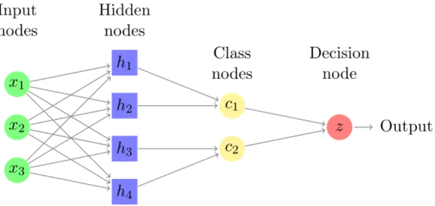
• Probabilistic Neuronal Network [2]: A probabilistic neural network (PNN) is pre-dominantly a classifier that maps any input pattern to a number of classifications. PNN can be forced into a more general function approximator.

x1 x2 x3 h1 h2 h3 h4 c1 c2 z Output Hidden nodes Class nodes Input nodes Decision node

Figure 2: Example of a Probabilistic Neuronal Network.

(14)

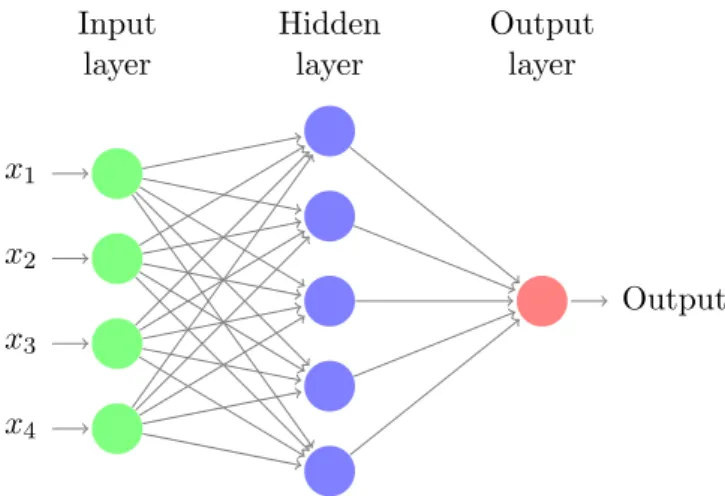
net-work (RProp) is an interconnection of nodes in which data and calculations flow in a single direction, from the input data to the outputs. The number of layers in a neural network is the number of layers of perceptrons.

x1 x2 x3 x4 Output Hidden layer Input layer Output layer

(15)

3 Behavior Recognition and Behavior Cloning from Observation

Having formally defined the tools employed in this project, we proceed by presenting the way we used them to achieve our goals.

3.1 Training a Probabilistic Finite Automaton

We propose to train a PFA A = (Σ, Q, φ, ι, γ) to model an unknown behavior by observ-ing its trace T . To this end, we define the alphabet Σ of automaton A to be the set of all actions Y that the agent can perform. The state space Q depends on the model: it is either X (Model 1), or X × X (Model 2) or X × Y × X (Model 3).

Training the automaton A from a trace T = [(x1, y1), (x2, y2), . . . , (xm, ym)] consists of determining the initial probability values {ι(q) | q ∈ Q} and the transition probability function values {φ(q, a, q0) | q, q0 ∈ Q, a ∈ Σ} (we opted for a model with no final probabilities). For any state q ∈ Q, let ]q be the number of occurrences of symbol q in trace T . Note that in the case of Model 1, ]q = |{i ∈ 1, m | xi = q}|, for Model 2, if q = (x, x0), then ]q = |{i ∈ 2, m | xi−1 = x, xi = x0}|, and for Model 3, if q = (x, y, x0), then ]q = |{i ∈ 2, m | xi−1 = x, yi−1 = y, xi = x0}| . Similarly, we define ](q, a) and ](q, a, q0) for a ∈ Σ and q, q0 ∈ Q as follows.

Model 1: q = x, a = y, q0= x0 ](q, a) = |{i ∈ 1, m | xi= x, yi = y}|

](q, a, q0) = |{i ∈ 1, m − 1 | xi = x, yi = y, xi+1= x0}| Model 2: q = (x00, x), a = y, q0= (x, x0)

](q, a) = |{i ∈ 2, m | xi−1= x00, xi= x, yi = y}|

](q, a, q0) = |{i ∈ 2, m − 1 | xi−1= x00, xi = x, xi+1= x0, yi = y}| Model 3: q = (x00, y00, x), a = y, q0 = (x, y, x0)

](q, a) = |{i ∈ 2, m | xi−1= x00, xi= x, yi−1= y00, yi= y}|

](q, a, q0) = |{i ∈ 2, m − 1 | xi−1= x00, xi = x, xi+1= x0, yi−1= y00, yi= y}|

Note that in the case of Models 2 and 3, ](q, a, q0) is zero by definition if the last element of state q is different than the first element of state q0. Next, we estimate the values of ι and φ with the following formulas (we use Laplace smoothing to avoid zero values in the testing phase for elements that never appeared in training).

ι(q) := ]q + 1 m + |Q| φ(q, a, q 0 ) := ](q, a, q 0_{) + 1} ]q + |Q| × |Σ|

(16)

It is easy to see that P(a | q) becomes (](q, a) + |Q|)/(]q + |Q| × |Σ|), and this is precisely the probability of performing the action a when in state q.

3.2 Evaluation Metrics

In order to evaluate our system, we used the evaluation metrics described below.

3.2.1 Evaluation Metrics for Behavior Recognition

In the case of Behavior Recognition, the goal is to identify which was the strategy used by the agent, given a learning trace T = [(x1, y1), . . . , (xm, ym)] . To this end, we train a PFA Ak for each available planned strategy, we compute the value PAk(α, π

M_{) and} return i := argmaxk{PAk(α, π

M_{)}, where α = (y}

1, . . . , ym) and πM = (qM1 , . . . , qmM). The value of q_iM depends on the amount M of memory used: q_i1 = xi for Model 1, q_i2= (xi, xi−1) for Model 2 and qi3= (xi, xi−1, yi−1) for Model 3.

Next we measure the distance between an unknown behavior B exhibited by agent A and a given behavior B0 modeled by automaton Ak by computing the negative log-probability RM_A k(T ) := − 1 mlog PAk(α, π M_), ₍₆₎

where T is the trace corresponding to behavior B and m is the number of observations in T . This value can be interpreted as a Monte Carlo approximation of the crossed entropy between behaviors B and B0, known in the literature as Vapnik’s risk (see [15]).

3.2.2 Evaluation Metrics for Behavior Cloning

We propose two methods for evaluating the performance of the cloning algorithms. Predictive Accuracy. This is a standard measure for classification tasks. Let M be the model trained by one of the learning algorithms using the trace obtained by observing an agent A (that follows a certain strategy) on a fixed set of maps. This model can be either deterministic (in which case, there is only one possible action at any point in time) or stochastic (the action is chosen randomly according to some probability distribution).

Now, let T = [(x1, y1), . . . , (xm, ym)] be the trace of the agent A on a different previously unseen map. The predictive accuracy AccM(T ) is measured as follows:

](M, T, i) = (

1 if M([xi−1, yi−1, ]xi) = yi

(17)

AccM(T ) = 1 n n X i=1 ](M, T, i) (8)

where M([xi−1, yi−1, ]xi) represents the action predicted by the model M for the state xi, possibly knowing previous state and action. If M is a stochastic model, M([xi−1, yi−1, ]xi) is a random variable over Y with the probability distribution {P(a | q)}a∈Y, where q = xi for Model 1, q = (xi, xi−1) for Model 2 and q = (xi, xi−1, yi−1) for Model 3.

Monte Carlo Distance.

To assess the quality with which a model M reproduces the behavior of an agent A we propose a Monte Carlo-like measure based on estimating the cross entropy between the probability distributions associated with both the model M and the agent A. We propose to estimate cross entropy from traces, for this reason it is a Monte Carlo estimation. More concretely, let T = [o1, . . . , on] be a trace generated2 according to model M on a fixed map (different than the one used in training), and let T0 = [o0₁, . . . , o0_m] be the trace generated by the agent on the same map. We define the Monte Carlo distance between model M and agent A as follows (estimated through traces T and T0):

H(T, T0) = −1 n n X i=1 log   1 m m X j=1 I{o0 j}(oi)   (9) Here I{o0

j} means the indicator function of set {o

0

j}. Obviously the previous measure in Equation (9) is empirical. It is assumed that for large enough traces it is closed to the true cross entropy between the behavior corresponding to model M and the behavior exhibited by agent A.

Using Laplace smoothing, the previous formula becomes:

H(T, T0) = −1 n n X i=1 log " Pm j=1I{o0 j}(oi) + 1 m + |X × Y| # (10)

2_{The model predicts the next action, but the next state is given by the actual configuration of the}

map; in the case that it is impossible to perform a certain action because of an obstacle, the agent does not change its location.

(18)

4 Experiments

We have run our experiments with a simulator of a simplified version of a Roomba, which is a series of autonomous robotic vacuum cleaners sold by iRobot3. The original Roomba vacuum cleaner uses a set of basic sensors that help it perform tasks. For instance, it is able to change direction whenever it encounters an obstacle. It uses two independently operating wheels that allow 360 turns in place. Additionally, it can adapt to perform other more creative tasks using an embedded computer in conjunction with the Roomba Open Interface.

4.1 Training Maps

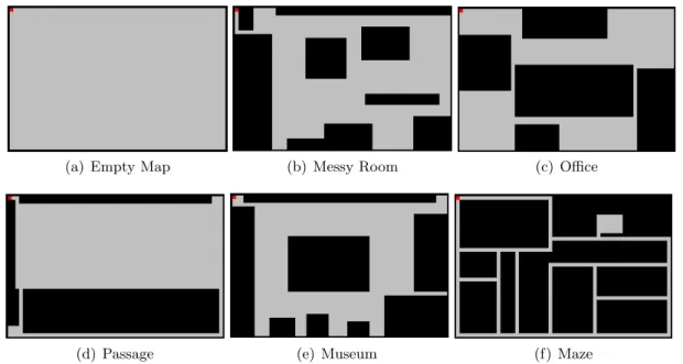
The environment in which the agent moves is a 40 x 60 rectangle surrounded by walls, which may contain all sorts of obstacles. For testing, we have randomly generated obstacles on an empty map. In the sequel, we briefly explain the six maps used in the training phase. Each of them is meant to represent a real-life situation, as indicated by their title (the list is by no means exhaustive).

(a) Empty Map (b) Messy Room (c) Office

(d) Passage (e) Museum (f) Maze

Figure 4: Training Maps

Empty Map. The empty map consists of a big empty room with no obstacles whatso-ever.

3

According to wikipedia, “iRobot Corporation is an American advanced technology company founded in 1990 and incorporated in Delaware in 2000. Roomba was introduced in 2002. As of Feb 2014, over 10 million units have been sold worldwide”.

(19)

Messy Room. The messy room simulates an untidy teenager bedroom, with all sorts of obstacles on the floor, and with a narrow entry corridor that makes the access to the room even more challenging for any ‘hostile intruder’.

The Office. The office map simulates a space in which several rooms are connected to each other by small passages. In this case, obstacles are representing big furniture such as office desks or storage cabinets.

The Passage. The highlight of this map is an intricate pathway that leads to a small room. The main room is huge and does not have any obstacle in it.

The Museum. This map is intended to simulate a room from a museum, with the main sculpture in the center, and with several other sculptures on the four sides of the room, separated by small spaces.

The Maze. The most part of this map consists of narrow pathways with the same width as the agent. There is also a little room which is difficult to find.

The six maps are represented in Figure 4.

4.2 Agent Strategies

We have designed a series of strategies with different complexities. When describing a strategy, we must define the behavior of the agent in a certain situation (which defines its state Xt) that depends on the configuration of obstacles in its vicinity (prefix Rnd is used for stochastic strategies).

Walk. The agent always performs the same movement in a given state. As an example, a possible strategy could be to go Right whenever there are no obstacles, and Up whenever there is only one obstacle to the right (stationary deterministic of type 2, it only depends on current state Xt).

Rnd Walk. In this strategy, the next move is picked up randomly from the set of available moves. For example, an agent that has obstacles to the right and to the left can only move Up or Down, but there is no predefined choice between those two (stationary stochastic of type 2, it only depends on current state Xt).

Crash. In this strategy the robot should perform the same action as in the previous cell while there exists this possibility. Whenever it encounters a new obstacle in its way, the agent must choose a certain predefined action. Therefore, it needs to have information about its previous action in order to know where to move (stationary deterministic of type 3, it depends on current state Xt and previous action Yt).

Rnd Crash. This strategy allows the agent to take a random direction when it crashes with an obstacle. The main difference with the Rnd Walk is that in Rnd Crash the agent does not change direction if it does not encounter an obstacle in its way (stationary stochastic of type 3, it depends on current state Xt and previous action Yt−1).

(20)

ZigZag. It consists of different vertical movements in two possible directions, avoiding the obstacles. It has an internal state which tells the robot if it should advance towards the left or the right side with this vertical movements: it initially goes towards the right side, and once it reaches one of the right corners, the internal state changes so that the robot will start moving toward the left side (stationary deterministic of type 3, it depends on current state Xt, previous action Yt−1 and internal state Ct).

Rnd ZigZag. This strategy is similar to the previous one, with the only difference that once it reaches a corner the internal state could either change its value or not, and this is randomly assigned (stationary stochastic of type 3, it depends on current state Xt, previous action Yt−1 and internal state Ct).

4.3 Traces and Performance Evaluation

In our experiments the simulation time is discrete, and at each time step, the agent can take one out of these 5 actions: up, down, left, right and stand still, with their intuitive effect (if the agent tries to move into an obstacle, the effect is equivalent to the stand still action). The control variable Y can take 5 different values: {Up, Down, Left, Right, Stand}. The agent perceives the world through the input variable X having 4 different binary components (up, down, left, right), one of them identifying what can the vacuum cleaner see in each direction (obstacle, no obstacle).

We work with an agent represented by a fairly simplified version of a Roomba robot. In our implementation, although it is possible for the agent to start anywhere, the traces we generate are always with the agent starting in the top-left corner of the map. We use the strategies explained in the section 4.2 and the maps described in section 4.1. For each pair map/strategy we have generated a trace of 1500 observations. In the training phase, we used, for each strategy, a single file obtained by concatenating the traces from the above mentioned six maps. Therefore, each machine was trained using 9000 observations coming from different types of maps.

4.4 Behavior Recognition Experimentation

In order to evaluate our behavior recognition system, we performed two experiments. We have randomly generated three maps (Testing Group 1) for the first experiment and 100 maps (Testing Group 2) for the second experiment. Then, we generated a family of traces (each of them containing 1500 observations) for each pair strategy/map: (T_ni)i∈{1,2,3},n∈{1,...,6}and ( ¯Tni)i∈{1,...,100},n∈{1,...,6}for the first and the second experiment, respectively.

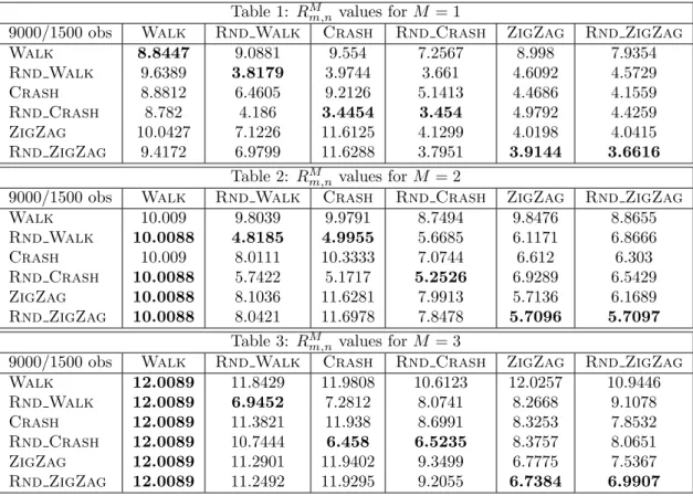
For the first experiment, we computed the log-normalized distance RM_A_m(T_ni) between the observation trace T_ni and the automaton Am, as described in Equation (6). The average value R_m,nM = P3

i=1RMAm(T

i

(21)

the (m, n)-th cell of Table M , with M in {1, 2, 3} corresponding to Model 1, Model 2 and Model 3, respectively. Our system classifies the testing task represented by column n as being generated by the automaton Ak such that k = argminmRMm,n (minimizing distance maximizes trace probability).

Table 1: RM_m,nvalues for M = 1

9000/1500 obs Walk Rnd Walk Crash Rnd Crash ZigZag Rnd ZigZag

Walk 8.8447 9.0881 9.554 7.2567 8.998 7.9354 Rnd Walk 9.6389 3.8179 3.9744 3.661 4.6092 4.5729 Crash 8.8812 6.4605 9.2126 5.1413 4.4686 4.1559 Rnd Crash 8.782 4.186 3.4454 3.454 4.9792 4.4259 ZigZag 10.0427 7.1226 11.6125 4.1299 4.0198 4.0415 Rnd ZigZag 9.4172 6.9799 11.6288 3.7951 3.9144 3.6616 Table 2: RM m,nvalues for M = 2

9000/1500 obs _Walk _{Rnd Walk} _Crash _{Rnd Crash} _ZigZag _{Rnd ZigZag}

Walk 10.009 9.8039 9.9791 8.7494 9.8476 8.8655 Rnd Walk 10.0088 4.8185 4.9955 5.6685 6.1171 6.8666 Crash 10.009 8.0111 10.3333 7.0744 6.612 6.303 Rnd Crash 10.0088 5.7422 5.1717 5.2526 6.9289 6.5429 ZigZag 10.0088 8.1036 11.6281 7.9913 5.7136 6.1689 Rnd ZigZag 10.0088 8.0421 11.6978 7.8478 5.7096 5.7097 Table 3: RM m,nvalues for M = 3

9000/1500 obs _Walk _{Rnd Walk} _Crash _{Rnd Crash} _ZigZag _{Rnd ZigZag} Walk 12.0089 11.8429 11.9808 10.6123 12.0257 10.9446 Rnd Walk 12.0089 6.9452 7.2812 8.0741 8.2668 9.1078 Crash 12.0089 11.3821 11.938 8.6991 8.3253 7.8532 Rnd Crash 12.0089 10.7444 6.458 6.5235 8.3757 8.0651 ZigZag 12.0089 11.2901 11.9402 9.3499 6.7775 7.5367 Rnd ZigZag 12.0089 11.2492 11.9295 9.2055 6.7384 6.9907

Figure 5: Distance Matrix for Testing Group 1

The results of this testing group show that the PFA recognition system is able to correctly recognize the three random strategies (Rnd Walk, Rnd Crash and Rnd ZigZag). However, the system fails when recognizing the respective underlying deterministic strategies (Walk, Crash and ZigZag). Also note that the deterministic versions of the random behaviors (Walk, Crash and ZigZag) are not confused one each other but each of them is most of the times classified by the system as its corresponding non deter-ministic version (Crash is classified as Rnd Crash, ZigZag as Rnd ZigZag). For the second experiment, the numerical value C_m,nM placed in the (m, n)-th cell of the confusion matrix is the empirical probability of the n-th task to be classified as the m-th task, that is, the percentage of the learning traces produced using strategy n that are recognized as being produced by strategy m.

(22)

More precisely, C_m,nM = |{i ∈ {1, . . . , 100} | m = argminkR M Ak( ¯T i n)}| 100

The diagonal of this matrix reflects the empirical probabilities of right classification and the sum of the other rows different from the diagonal element is the probability of error. We observe that this second experiment confirms the conclusions of the first one.

Table 1: CM

m,nvalues for M = 1

9000/1500 obs _Walk _{Rnd Walk} _Crash _{Rnd Crash} _ZigZag _{Rnd ZigZag}

Walk 0.13 0 0 0 0 0 Rnd Walk 0.27 1 0.07 0 0 0 Crash 0.2 0 0.2 0 0 0 Rnd Crash 0.4 0 0.53 1 0 0 ZigZag 0 0 0 0 0 0 Rnd ZigZag 0 0 0.2 0 1 1

Table 2: Cm,nM values for M = 2

Det Walk 0.27 0 0 0 0 0 Rnd Walk 0.27 1 0.27 0 0 0 Crash 0.53 0 0.2 0 0 0 Rnd Crash 0.33 0 0.47 1 0 0 ZigZag 0.13 0 0 0 0.2 0 Rnd ZigZag 0.13 0 0.07 0 0.8 1 Table 3: CM m,nvalues for M = 3

Walk 0.33 0 0 0 0 0 Rnd Walk 0.27 1 0 0 0 0 Crash 0.6 0 0.2 0 0 0 Rnd Crash 0.4 0 0.73 1 0 0 ZigZag 0.13 0 0 0 0.2 0 Rnd ZigZag 0.13 0 0.07 0 0.8 1

Figure 6: Confusion Matrix for Testing Group 2

4.5 Behavior Cloning Experimentation

As already mentioned, we used a file of 9000 observations for each strategy in order to train our models. For testing, we used again the three maps of Testing Group 1.

4.5.1 Predictive Accuracy.

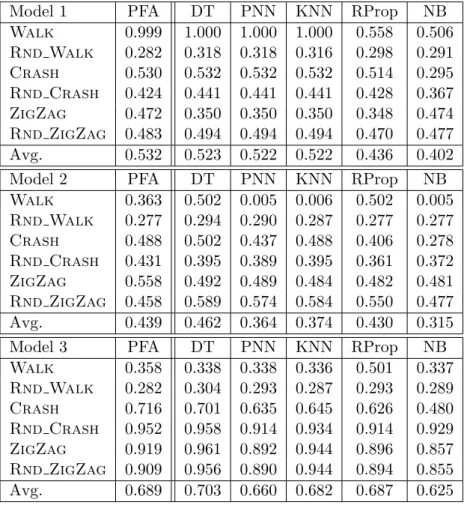
The numbers in the three tables of Figure 7 represent average values of the predictive accuracy (defined as in Equation (8)) computed for each of the three randomly generated

(23)

maps in Testing Group 1. Note that the only stochastic model is the PFA.

Model 1 PFA DT PNN KNN RProp NB

Walk 0.999 1.000 1.000 1.000 0.558 0.506 Rnd Walk 0.282 0.318 0.318 0.316 0.298 0.291 Crash 0.530 0.532 0.532 0.532 0.514 0.295 Rnd Crash 0.424 0.441 0.441 0.441 0.428 0.367 ZigZag 0.472 0.350 0.350 0.350 0.348 0.474 Rnd ZigZag 0.483 0.494 0.494 0.494 0.470 0.477 Avg. 0.532 0.523 0.522 0.522 0.436 0.402

Figure 7: Predictive Accuracy for the generated maps.

Analyzing the results, we can see that our hierarchy of models behaves as expected: type 3 behavior is very well captured by Model 3 (the one that uses information about both previous state and previous action), while type 2 behavior is better explained by Model 1 (in which we only take into account the current state). Note that even though intuitively, the more info we have, the best we can predict, in the case of type 2 behavior, using this extra information can do more harm than good. Another anticipated result that was experimentally confirmed is that Model 1 would be very good in predicting the Walk strategy, because the agent always performs the same action in a given state, and that Rnd Walk would be the most unpredictable strategy of all (a notable exception is in the case of Model 2, for which, surprisingly, PNNs and KNNs have even worse accuracy for the Walk strategy).

It is noteworthy the high accuracy rates of Model 3 for Rnd Crash, ZigZag and Rnd ZigZag, all type 3 strategies. Also, this model gives somewhat lower, but still good enough, prediction rates for the Crash strategy.

(24)

If we were to chose a classifier, we would opt for DTs, which gives, with only one exception (Model 3, Walk), best results among deterministic models.

Using a PFA is, most of the times, either the best option, or very close to the best one, especially when predicting the behavior of more complex strategies. Note that PFAs are notably better for describing type 3 behaviors. Also, although intuitively a stochastic model should be better than a deterministic model in describing the behavior of a random process, in our experiments, this is not the case (PFAs outperform DTs mostly when learning deterministic strategies).

4.5.2 Monte Carlo Distance.

In order to compare the distance between the agent’s behavior and the behavior of a given learned strategy, we used the same three randomly generated maps of Testing Group 1. For each of the classifiers (DT, PNN, KNN, RProp, NB) and for each of the six prede-fined strategies (Walk, Rnd Walk, Crash, Rnd Crash, ZigZag, Rnd ZigZag), we generated the trace T produced by an agent whose next action is dictated by the clas-sifier on each of the three randomly generated maps. On the other hand, we generated the trace T0 of each of the six predefined strategies on those three maps. In Figure 8 we present the average of H(T, T0) for each pair classifier/strategy (see Equation (10)). For stochastic models, the next action, instead of being predefined, is obtained by sampling according to the probability distribution given by the trained model.

Walk 0.752 0.752 0.752 0.752 7.348 7.348 Rnd Walk 4.562 7.027 7.027 7.027 7.315 7.315 Crash 1.441 3.877 3.877 3.877 7.348 7.348 Rnd Crash 5.349 6.734 6.734 6.734 7.352 7.352 ZigZag 1.774 4.863 4.863 4.863 7.322 7.322 Rnd ZigZag 1.796 6.926 6.926 6.926 7.325 7.325 Avg. 2.612 5.030 5.030 5.030 7.335 7.335 Figure 8: Monte Carlo distance between original and cloned behavior

Analyzing the results, we can see that PFAs are the best in cloning the agent’s behavior for all six strategies, and that the deterministic approach only equals its performance for the Walk strategy. Also note that random behaviors are harder to reproduce than their deterministic counterparts.

(25)

5 Implementation

Now we will go through each of the steps followed in the implementation phase of this project, specifying the programming languages and the software used, and explaining the relationship between the JAVA code, the PFA Python files and the KNIME work-flow.

5.1 JAVA Programming Language

The decision of choosing JAVA has been made based on several considerations. First, it is an object oriented language. Secondly, it is a language that gives you plenty of flexibility when it comes to upgrading the code, and lastly, it is a cross-platform and an open-source programming language. There are also lots of libraries and packages that allow its use in a comfortable way, with all the information about JAVA on the Internet.

Step One

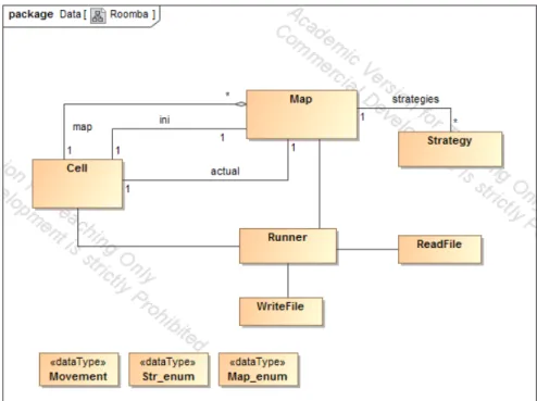
The first implemented system consists of a map of cells, each of them being defined by its coordinates. The “Cell” class in the beginning was composed of the getter and setter methods for its coordinates.

Another component of this first system is the environment, which consists of a group of cells that compose a map. That map is created in a class named “Map”, structured as a matrix of 60x40 cells. In the “Map” class, we have to set an initial cell to know where the agent begins its route. In addition, it is necessary to set the position of the agent in a determinate moment, so we created the attribute “actual” in the “Map” class. This gives us an empty map for the agent, in which we needed to add some obstacles. On one hand, we created the walls to prevent the agent from escaping the map with a method call “addWalls”. On the other hand, we created difficulties in the movement of the agent around the map by generating a number of obstacles that will appear on the map with the method “addObstacle”.

After adding the obstacles, the agent has to know where are its surrounding cells, if they are obstacles or not, and to know where to go according to its strategy. We have added a method for each of the situations in which the robot can be found, and which returns a Boolean value indicating whether the agent finds itself in that situation. For example, if we want to know if the agent has an obstacle on its right cell, we have to call the method “isObstacleRight”.

In some cases, it is important to know which was the last movement of the agent, so we added a “Movement” object that reflects it. This attribute is important because most of the strategies need to know the agent’s last movement.

(26)

We also created a class named “Strategy” containing all the agent’s predefined strategies. For each strategy, we created a method that tells the agent what to do in any possible situation. In this class we also have a method that chooses which strategy should the agent follow. This method is called “selectStrategy” and it has two parameters:

• Strategy: We choose one of the enumerate values from the class “Str enum”. • Movement: We have to pass the last movement of the agent to this method. The

movement is also an enumerate value, in this case from the class “Movement”. Because of the obstacles present in the maps, we needed to include a new attribute in the “Cell” class that defines the cell as a possible obstacle. As we did for the coordinates, we created a getter and setter method for the Boolean attribute obstacle. In addition, we added another Boolean value that allows us to know if one cell has been visited by the agent (this is useful for strategies that depend on all previously visited cells). In the “Map” class we created six maps with the same dimension, where the agent can follow any possible strategy. We created the “selectMap” method, where we generate each of the maps by adding obstacles. For choosing the map we want, we have to set a “Map enum” object as a parameter. The “Map enum” class is composed by enumerate values, each of them representing one of the maps that we created in the “selectMap” method.

So far, the agent can move around the map following one of the strategies and avoiding obstacles.

Step Two

In a second iteration, we decided to add the possibility of generating random maps. We do so by adding a method in “Map” class that consists of given the number of obstacles we want to add, we distribute all of them around the map, obtaining a random map. Each time we use this method we obtain a different map. These random maps will be used to obtain testing sets of the movement of the agent following an strategy.

One utility that was missing in Step One was the ability of exporting information about the agent to a CSV file. According to the models of section 2, we have to export different information about the agent as it is said in Figure 1. We create the “WriteFile” class when we use the package “java.io” that help us with the input and output file system.

In this class we have two methods:

• “WriteIn”: This method consists of writing one CSV file per strategy with the movements of the agent. We will write 1500 observations per map, totaling 9000 observations, for all the strategies. These CSV files form the training set.

• “WriteTesting”: We write one CSV file per strategy according to the movements of the agent in a random map. This file will be used in Python or Knime as a testing set for a strategy.

(27)

After creating these CSV files we used them to train and test our models as specified in Section 4.

Step Three

The necessity of using generated random maps more than one time meant that we needed to implement a method that exports a map to a text file. This method exports the information of the whole map in a CSV file where each line represents one cell, identified by its coordinates. This method will appear in the “WriteFile” class as “writeMap” and it is necessary to pass a “Map” object as a parameter.

Apart from exporting information from the agent, we also want to be able to import information for a strategy (in Behavioral Cloning, for example). We created a new class named “ReadFile”. Using again the “java.io” package we could import the results obtained from the PFA and the classifiers to make new strategies. These new strategies will be implemented in “Strategy” class in the two methods where we have to pass as parameter a link to the CSV file that contains the strategy. In the “ReadFile” class we can also import a map from a CSV file. We need this method in order to use a random map more than once.

Finally, we obtain the following class diagram that is a brief representation of our JAVA project.

(28)

5.2 Python Programming Language

Python is a concise and compact dynamically typed programming language, which makes it much easier to use than JAVA. It promotes the use of functions, which are equivalent to JAVA methods. We used it to train the Probabilistic Final Automaton and to evaluate the models obtained as described in section 3.2. Also, all tables were automatically generated in Python.

Concretely, we implemented a function to import all the observations of the agent from the CSV files. When we import our data, we have to take into account which of the three models is used (see Section 2).

After importing all the observations, we implement a function that trains a PFA and another one that computes the probability of a given trace to have been generated by that PFA according to the formulas that appear in Section 2.1. Also, we implement functions that allow us to compute the Predictive Accuracy of Figure 7 and the Monte Carlo distance values of Figure 8.

5.3 Knime Analytics Platform

KNIME is a data mining tool that allows us to get, for each one of the models, the range of successful predictions of the next move of the agent according to its state, using the classifiers mentioned in section 2.1. It is an open source and licensed software, and also the tool used in the course of Machine Learning and Data Mining for the final project, which made it a perfect candidate for accomplishing this task.

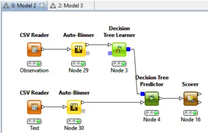
KNIME projects are composed by nodes. Each node is defined and properly explained in KNIME, so it is easy to know which node serves for each task. To import the observations of the agent that we extract from the JAVA project, we use a node called “CSV Reader”. This node generates a database with all the information that appears in the CSV file.

For each one of the classifiers, we used two nodes “CSV Reader” because one is dedicated to training and the other for testing. After that, we have to classify the movement that the agent will do (from 1 to 4); most of the classifiers used String variables, so we had to group the values we wanted to classify from the database in sets composed by Strings; for example, the number 1 will be in the “Bin 1”. For this operation in KNIME we used a node called “Auto Binner”.

Then, after having all the database ready for prediction, we used different classifiers. Most of them are composed by two related nodes: a “Learner” node and a “Predictor” node. Training sets will go to the “Learner” node to train the classifier and testing values go to the “Predictor” node. Finally, we use the “Score” node to obtain the accuracy of the classifier, which tells us whether the classifier works properly. The values obtained are reported in Figures 7 and 8.

(29)

In the sequel we show the scheme of the KNIME workflow used for Decision Trees. The other workflows are very similar to this one.

(30)

6 Concluding Remarks and Future Work

The realization of this project has given me great satisfactions at both professional and personal level. On one hand, all proposed objectives defined were accomplished.

We have proposed a model for behavior recognition. Behaviors are identified with tasks (or strategies for solving a given problem). Our system uses PFAs and correctly identifies tasks performed by the actor whenever those tasks have a certain random component. One of the strengths of our system is that it captures the stochastic aspects of behaviors. On the other hand, another characteristic of our model is the difficulty to distinguish between a certain strategy and a similar strategy perturbed with some degree of ran-domness. The inference technique is based on the greatest likelihood probability value generated by the PFAs of the model. The major computational limitation in our fully observable state space is the amount of memory required by the trained automaton. A possible solution is to employ only a few amount of non-observable internal states. An-other possible approach is the use of some notion of context learning in order to reduce the number of possible states.

We have proposed several models for behavior cloning and two evaluation metrics. First, we used ML classifiers to predict the action of the agent in a given state (a deterministic model). Then, we trained a PFA to estimate the probabilities of the agent’s actions in a given state (a stochastic model). In both cases, we measured the predictive accu-racy on new unseen data: deterministic approaches turned out to give slightly better results, but the difference was negligible. Nevertheless, when comparing the trace of the learned strategy with the trace of the original agent on a randomly generated map, we could experimentally check that PFAs do a better job than any of the classifiers under study.

On the other hand, this project has given me the opportunity to deepen my knowledge in machine learning and data mining.

Finally, at a personal level, this work lead to my debuting in scientific writing by con-tributing to two conference articles, accepted for publication at CAEPIA 2015 [11] and at UCAmI 2015 [22] as LNCS proceedings.

We plan to extend this methodology to a more realistic type of robot, which can perform rotations of different angles and whose position is represented by real values on the map. Moreover, the set of agent’s strategies should be extended to include non-stationary type behaviors and other more sophisticated behaviors, such as the outward-moving spiral of the Roomba robot. Future work also contemplates the usage of probabilistic transducers, to take into account the input-output (state-action) nature of the observations composing the learning traces in the observation scenario. Finally, another future work direction is getting our models to deal with a greater fixed amount of memory, with the obvious computational limitation induced by our fully observable state space, which is directly proportional with the amount of memory required by the trained automaton.

(31)

References

[1] Bauer, M.A.: Programming by examples. Artif. Intell. 12(1), 1–21 (1979), http: //dx.doi.org/10.1016/0004-3702(79)90002-X

[2] Berthold, M.R., Diamond, J.: Constructive training of probabilistic neural net-works. Neurocomputing 19(1-3), 167–183 (1998), http://dx.doi.org/10.1016/ S0925-2312(97)00063-5

[3] Dupont, P., Denis, F., Esposito, Y.: Links between probabilistic automata and hidden markov models: probability distributions, learning models and induction algorithms. Pattern Recognition 38(9), 1349–1371 (2005)

[4] Fernlund, H.K.G., Gonzalez, A.J., Georgiopoulos, M., DeMara, R.F.: Learn-ing tactical human behavior through observation of human performance. IEEE Transactions on Systems, Man, and Cybernetics, Part B 36(1), 128–140 (2006),

http://doi.ieeecomputersociety.org/10.1109/TSMCB.2005.855568

[5] Floyd, M.W., Esfandiari, B., Lam, K.: A case-based reasoning approach to im-itating robocup players. In: Wilson, D., Lane, H.C. (eds.) Proceedings of the 21st International Florida Artificial Intelligence Research Society Conference, May 15-17, 2008, Coconut Grove, Florida, USA. pp. 251–256. AAAI Press (2008),

http://www.aaai.org/Library/FLAIRS/2008/flairs08-064.php

[6] Gonzalez, A.J., Georgiopoulos, M., DeMara, R.F., Henninger, A., Gerber, W.: Au-tomating the CGF model development and refinement process by observing expert behavior in a simulation. In: Proceedings of The 7th Conference on Computer Generated Forces and Behavioral Representation (1998)

[7] Han, J., Kamber, M., Pei, J.: Data mining: concepts and techniques: concepts and techniques. Elsevier (2011)

[8] K¨onik, T., Laird, J.E.: Learning goal hierarchies from structured observations and expert annotations. Machine Learning 64(1-3), 263–287 (2006), http://dx.doi. org/10.1007/s10994-006-7734-8

[9] Lozano-P´erez, T.: Robot programming. In: Proceedings of IEEE. vol. 71, pp. 821– 841 (1983)

[10] Michalski, R.S., Stepp, R.E.: Learning from observation: Conceptual clustering. In: Michalski, R.S., Carbonell, J.G., Mitchell, T.M. (eds.) Machine Learning: An Artificial Intelligence Approach, chap. 11, pp. 331–364. Tioga (1983)

[11] Montaña, J.L., Tˆırn˘auc˘a, C., Sobremazas, C.O., Ontañón, S.: A probabilistic au-tomata framework for behavioral recognition. In: Actas de la XVI Conferencia de la Asociación Española para la Inteligencia Artificial (CAEPIA 2015), November 9-12, Albacete, Spain (To appear) (2015)

(32)

[12] Moriarty, C.L., Gonzalez, A.J.: Learning human behavior from observation for gaming applications. In: Lane, H.C., Guesgen, H.W. (eds.) Proceedings of the 22nd International Florida Artificial Intelligence Research Society Conference, May 19-21, 2009, Sanibel Island, Florida, USA. AAAI Press (2009), http://aaai.org/ ocs/index.php/FLAIRS/2009/paper/view/100

[13] Ng, A.Y., Russell, S.: Algorithms for Inverse Reinforcement Learning. In: in Proc. 17th International Conf. on Machine Learning. pp. 663–670 (2000)

[14] Onta˜n´on, S., Mishra, K., Sugandh, N., Ram, A.: On-line case-based planning. Computational Intelligence 26(1), 84–119 (2010), http://dx.doi.org/10.1111/ j.1467-8640.2009.00344.x

[15] Ontañón, S., Montaña, J.L., Gonzalez, A.J.: A dynamic-bayesian network frame-work for modeling and evaluating learning from observation. Expert Systems with Applications 41(11), 5212–5226 (2014)

[16] Pomerleau, D.: ALVINN: An autonomous land vehicle in a neural network. In: Touretzky, D.S. (ed.) Advances in Neural Information Processing Systems 1 (NIPS 1998). pp. 305–313. Morgan Kaufmann (1988), http://papers.nips.cc/paper/ 95-alvinn-an-autonomous-land-vehicle-in-a-neural-network

[17] Rabin, M.O.: Probabilistic automata. Information and Control 6(3), 230–245 (1963) [18] Riedmiller, M., Braun, H.: A direct adaptive method for faster backpropagation learning: the RPROP algorithm. In: IEEE International Conference on Neural Networks. vol. 1, pp. 586–591. IEEE (1993), http://dx.doi.org/10.1109/icnn. 1993.298623

[19] Sammut, C., Hurst, S., Kedzier, D., Michie, D.: Learning to fly. In: Sleeman, D.H., Edwards, P. (eds.) Proceedings of the 9th International Workshop on Machine Learning, July 1-3, 1992, Aberdeen, Scotland, UK. pp. 385–393. Morgan Kaufmann (1992)

[20] Shafer, J.C., Agrawal, R., Mehta, M.: SPRINT: A scalable parallel classifier for data mining. In: Vijayaraman, T.M., Buchmann, A.P., Mohan, C., Sarda, N.L. (eds.) Proceedings of 22th International Conference on Very Large Data Bases, September 3-6, 1996, Mumbai (Bombay), India. pp. 544–555. Morgan Kaufmann (1996),http://www.vldb.org/conf/1996/P544.PDF

[21] Sidani, T.: Automated Machine Learning from Observation of Simulation. Ph.D. thesis, University of Central Florida (1994)

[22] Tˆırn˘auc˘a, C., Montaña, J.L., Sobremazas, C.O., Ontañón, S., González, A.J.: Teaching a virtual robot to perform tasks by learning from observation. In: Pro-ceedings of the 9th International Conference on Ubiquitous Computing & Ambient Intelligence (UCAmI 2015), December 1-4, Puerto Varas, Chile (To appear) (2015)