An Analysis of Some Algorithms and Heuristics for Multiobjective Graph Search

(1)

An Analysis of Some Algorithms and

Heuristics for Multiobjective Graph

Search

TESIS DOCTORAL

Enrique L. Machuca Sánchez

Universidad de Málaga

(2)

(3)

An Analysis of Some Algorithms and

Heuristics for Multiobjective Graph

Search

Memoria que presenta el doctorando

Enrique L. Machuca Sánchez

para optar al grado académico de Doctor Ingeniero en Informática

Dirigida por el Doctor

Lorenzo Mandow Andaluz

Departamento de Lenguajes y Ciencias de la Computación Escuela Técnica Superior de Ingeniería Informática

Universidad de Málaga

24 de Julio de 2012

Tribunal de la tesis / Thesis Committee

Dr. José Luis Pérez de la Cruz Molina - Universidad de Málaga Dra. Amparo Ruiz Sepúlveda- Universidad de Málaga

Dra. Raquel Fuentetaja Pizán - Universidad Carlos III de Madrid Dra. Lucie Galand - Université Paris Dauphine

Dra. Camino Rodríguez Vela - Universidad de Oviedo

Evaluadores externos / External Reviewers

(4)

E-MAIL: [email protected]

WWW:http://www.lcc.uma.es/~machuca

This work is licensed under a Creative Commons Attribution-NonCommercial-NoDerivs License: http://creativecommons.org/licenses/by-nc-nd/3.0/

This work is partially funded by/Este trabajo está financiado por:

Consejería de Economía, Innovación, Ciencia y Empresa. Junta de Andalucía (España)

(5)

El Dr. D. Lorenzo Mandow Andaluz, Profesor Titular de Universidad, del Área de Ciencias de la Computación e Inteligencia Artificial de la Escuela Técnica Superior de Ingeniería Informática de la Universidad de Málaga,

Certifica que,

D. Enrique L. Machuca Sánchez, Ingeniero en Informática, ha realizado en el Depar-tamento de Lenguajes y Ciencias de la Computación de la Universidad de Málaga, bajo su dirección, el trabajo de investigación correspondiente a su Tesis Doctoral titulada:

An Analysis of Some Algorithms and Heuristics for Multiobjective Graph Search

Revisado el presente trabajo, estima que puede ser presentado al tribunal que ha de juzgarlo, y autoriza la presentación de esta Tesis Doctoral en la Universidad de Málaga.

Fdo.: Dr. Lorenzo Mandow Andaluz

(6)

(7)

(8)

(9)

Agradecimientos

Aunque sea la primera quizás en leer, esta es la última página que escribo, y con ella quiero agradecer de corazón su aprecio, su apoyo y su ayuda a cuantos han hecho posible que este trabajo de tesis doctoral sea una realidad.

En primer lugar, a mi director de tesis, Lawrence, que me ha guiado siempre y en cada momento hacia la meta, con más tenacidad de la que yo he sabido mostrar en muchos momentos. Ha sido mi maestro y mi mentor, pero también agradezco enormemente su gran humanidad, su comprensión y apoyo siempre ante situaciones personales. Ojalá haya adquirido en estos años todas las dotes y habilidades que tan amablemente ha sabido mostrarme para esta ardua tarea de ser científico y poder aportar mi granito de arena al conocimiento de la humanidad.

Por supuesto también a Pepe Luis, al que debo también mi aprendizaje gracias a sus siempre sabias críticas y consejos. Es una suerte haber disfrutado de la opinión y el apoyo de otro gran científico. Compañeros de viaje también han sido Amparo, Javier y mi compañero Francis, entre otros, con los que he podido compartir mis debates sobre NAMOA, la búsqueda heurística o la investigación en general. Es de bien nacido ser agradecido, así que no quiero dejar pasar la ocasión para dar las gracias a la Junta de Andalucía por concederme una beca de investigación (ref. P07-TIC-03018), y por ende a tod@s los andaluces, por hacer realidad este deseo de ser Doctor y llegar al máximo nivel de conocimiento en una disciplina científica.

No quiero olvidarme del Dr. Sanders, la Dra. Wagner y todas las personas que allí en Karlsruhe me acogieron y me ayudaron; también ha sido una interesante experiencia. Entre ellos, no puedo dejar de mencionar a mi querido amigo Alex, a quien siempre llevaré en el corazón. También he de dar las gracias a aquellos investigadores con los que he podido debatir o colaborar de alguna manera en estos años, como la Dra. Raith, el Dr. Iovanella, el Dr. Edelkamp o el Dr. Zaroliagis.

Pero aparte de trabajo, también han sido años de compartir experiencias muy pos-itivas en lo personal, y no quisiera olvidarme de cuantas personas han sufrido mis conversaciones, mis bromas o mis emails en el laboratorio. No voy a nombrar a tod@s porque son much@s, y a cada cual los llevaré siempre en el recuerdo. Pero especial-mente tengo que nombrar a Jaime, mi querido compañero de viaje, con el que comparto las penas y las alegrías de esta sufrida profesión, y al que me une, más que trabajo, una gran amistad.

He de recordar también que hasta aquí no habría llegado si no fuera por lo que aprendí de profesores de Universidad, como mi tutor de PFC Edu, de compañer@s y profesor@s de departamento, o de las grandes personas que me formaron en el colegio San José. También debo mi gratitud y mi recuerdo a aquellas personas que marcaron

(10)

de alguna manera mi personalidad y con las que he compartido tantos momentos de mi vida, compañer@s de clase, de facultad, amig@s, herman@s de fe y familiares, que diré simplemente que son muchos y muy queridos para mí, para no menospreciar a unos y olvidar a otros.

Y por último, a Sarai por sufrir las consecuencias de ser científico en este mundo tan complicado que vivimos, y a mi familia, por darme lo que soy en esta vida, y por mostrarme el camino hacia Dios y hacia los hombres. De ellos recibí el amor, y aprendí a ser mejor persona, a tener unos valores y unos sentimientos que conforman en gran manera lo que soy.

A tod@s, en este momento tan importante de mi vida, de corazón, ¡¡GRACIAS!!

(11)

Abstract

Many real problems require the examination of an exponential number of alternatives in order to find the best choice. They are the so-called combinatorial optimization problems. Besides, real problems usually involve the consideration of several conflicting magnitudes. When multiple objectives must be simultaneously optimized, there is generally not an optimal value satisfying the requirements for all the criteria at the same time. Solving these multiobjective combinatorial problems commonly results in a large set of Pareto-optimal solutions, which define the optimal tradeoffs between the objectives under consideration.

One of most recurrent multiobjective problems is considered in this thesis: the search for shortest paths in a graph, taking into account several objectives at the same time. Many practical applications of multiobjective search in different domains can be pointed out: routing in multimedia networks (Clímaco et al., 2003), satellite scheduling (Gabrel & Vanderpooten, 2002), transportation problems (Pallottino & Scutellà, 1998), routing in railway networks (Müller-Hannemann & Weihe, 2006), route planning in road maps (Jozefowiez et al., 2008), robot surveillance (delle Fave et al., 2009) or domain independent planning (Refanidis & Vlahavas, 2003).

Multiobjective route planning over realistic road maps has been considered as a po-tential application scenario for the multiobjective algorithms and heuristics considered in this thesis. Hazardous material transportation (Erkut et al., 2007), another related multiobjective routing problem, has also been considered as an interesting potential application scenario.

Single criterion shortest path methods are well known and have been widely studied. Heuristic Search allows the reduction of the space and time requirements of these me-thods, exploiting estimates of the actual distance to the goal. Multiobjective problems are much more complex than their single-objective counterparts, and require specific methods. These range from exact solution techniques to approximate ones, including the metaheuristic approximate methods usually found in the literature. This thesis is concerned with exact best-first algorithms, and particularly, with the use of heuristic information to improve their performance.

This thesis contributes both formal and empirical analysis of algorithms and heuris-tics for multiobjective search. The formal characterization of algorithms is important for the field. However, empirical evaluation is also of great importance for the real application of these methods. Several well known classes of problems have been used to test their performance, including some realistic scenarios as described above.

The results of this thesis provide a better understanding of which of the available methods are better in practical situations. Formal and empirical explanations of their

(12)

(13)

List of Figures

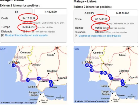
1.1 Screenshots from a sample route planning application, showing

alterna-tive routes from Málaga to Lisbon. . . 4

2.1 Supported, nonsupported and dominated points in a biobjective cost space 16 2.2 A sample graph with some nondominated solution paths and equivalent solutions . . . 19

2.3 The advantage of multiobjective pathmax (Dasgupta et al., 1999) . . . . 38

2.4 Multiobjective pathmax can not avoid the expansion of some dominated paths . . . 39

3.1 Rendering of the New York City map. . . 53

3.2 Rendering of primary (toll) highways of the New York City map. . . 55

3.3 Geo-referenced graph of the Lazio region in Italy. . . 57

4.1 Graph M C(2) . . . 71

4.2 Nondominated costs of paths in Graph M C(2) . . . 72

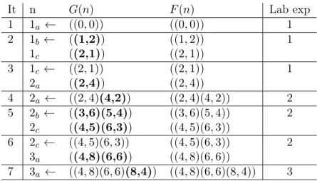
4.3 Label expansions of M OA∗ in graph M C(10) for different degrees of heuristic precision. Nodes are selected lexicographically, and values are shown for two different tie breaking rules. . . 78

5.1 Relative performance betweenM OA∗ andN AM OA∗ on class I/II grid problems with different correlation values (blind search) . . . 86

5.2 Estimated parameter values for the model rp =α∗sβ in the statistical analysis of the relative performance betweenM OA∗ andN AM OA∗ on class I/II grid problems with different correlation values (blind search) . 88 5.3 Performance of blind and heuristic N AM OA∗ search on class I grid problems. Average values over ten problems generated for each depth. . 92

5.4 Performance of blind and heuristic M OA∗ search on class I grid pro-blems. Average values over ten problems generated for each depth. Val-ues are not displayed when at least one problem exceeded a 1h runtime limit. . . 93

5.5 Performance of blind and heuristic N AM OA∗ search on class II grid problems. Average values over ten problems generated for each depth. . 94

5.6 Performance of blind and heuristic M OA∗ search on class II grid pro-blems. Average values over ten problems generated for each depth. . . . 95

(20)

5.7 Relative performance between M OA∗ and N AM OA∗ on class I grid problems with different correlation values (heuristic search) . . . 97 5.8 Relative performance between M OA∗ andN AM OA∗ on class II grid

problems with different correlation values (heuristic search) . . . 98 5.9 Performance of T C and heuristic N AM OA∗ search on class I grid

problems. Average values over ten problems generated for each depth. . 100 5.10 Performance of T C and heuristic N AM OA∗ search on class II grid

problems. Average values over ten problems generated for each depth. . 101 5.11 Time devoted to heuristics precalculation byT C and heuristicN AM OA∗/

M OA∗ on class I/II grid problems. Average values over ten problems generated for each depth. . . 103 5.12 Number of label expansions per node performed by blind and heuristic

N AM OA∗ in a sample 80×80 class II grid problem with ρ= 0. Start

node is (40,40)and goal node is (20,20). . . 107 5.13 Number of label expansions per node performed by blind and heuristic

M OA∗ in a sample80×80 class II grid problem withρ= 0. Start node is (40,40)and goal node is(20,20). . . 108 5.14 Number of superfluous label expansions per node performed by blind

M OA∗ in a sample 80×80 class II grid problem with ρ= 0. . . 109 5.15 Averages of different classes of label expansions per node depth

per-formed by blind M OA∗ in a sample 80×80 class II grid problem with

ρ= 0. . . 110 5.16 Number of superfluous label expansions per node performed by heuristic

M OA∗ in a sample 80×80 class II grid problem with ρ= 0. . . 112 5.17 Averages of different classes of label expansions per node depth

per-formed by heuristic M OA∗ in a sample 80×80 class II grid problem withρ= 0. . . 113 5.18 Dominance checks performed by blind and heuristic N AM OA∗ search

for class I grid problems. Average values over ten problems generated for each depth. . . 115 5.19 Dominance checks performed by T C and heuristic N AM OA∗ search

for class I grid problems. Average values over ten problems generated for each depth. . . 116 5.20 Percentage of filtering dominance checks among total (pruning and

fil-tering) dominance checks for class I grid problems with ρ= 0. . . 117 5.21 Dominance checks performed by blind and heuristic M OA∗ search for

class I grid problems. Average values over ten problems generated for each depth. Values are not displayed when at least one problem exceeded a 1h runtime limit. . . 118 5.22 Analysis on the time performance of T C and N AM OA∗ on a sample

100×100class I grid problem withρ= 0. . . 120 5.23 Time requirements for N AM OA∗ and T C to reach the first solution

(21)

List of Figures xxi

5.24 Performance of blind and heuristic search on DC road map problems. Average values over ten runs for each problem instance. . . 122 5.25 Performance of blind and heuristic search on RI road map problems.

Average values over ten runs for each problem instance. . . 123 5.26 Performance of blind and heuristic search on NJ road map problems.

Average values over ten runs for each problem instance. Values exceeding a 1h time limit are not displayed. . . 124

6.1 A typical Pareto-front in cost space . . . 135 6.2 Time requirements forN AM OA∗ with blind and heuristic search in NY

map . . . 136 6.3 Time requirements for N AM OA∗ with blind and heuristic search in

BAY map . . . 137 6.4 Time requirements for N AM OA∗ with blind and heuristic search in

COL map . . . 138 6.5 Time requirements for N AM OA∗ with blind and heuristic search in

FLA map . . . 139 6.6 Iterations performed by N AM OA∗ with the original and bounded

me-thods for the TC heuristic on NY problem instances. . . 147 6.7 Time requirements for N AM OA∗ with blind and heuristic search and

T C with heuristic selection inN Y2 map . . . 151

7.1 Improving~h_{T C} with two more informed estimates for some noden . . . 163 7.2 Non-supported solutions can not be found solving weighted sum problems164 7.3 Visual description of KDLS procedure . . . 165 7.4 A new solution is found in interval [C,B] while no more supported

solu-tions are found in interval [A,C] . . . 166 7.5 Sample graph for KDLS procedure: initialization . . . 169 7.6 Sample graph forKDLS procedure: searching for extreme solution costs 170 7.7 Sample graph for KDLS procedure: searching for supported solution

costs . . . 171 7.8 Sample graph forKDLS procedure: supported and non-supported

so-lution costs . . . 172 7.9 Space and time requirements for N AM OA∗∗ withH_KDLSk on class II

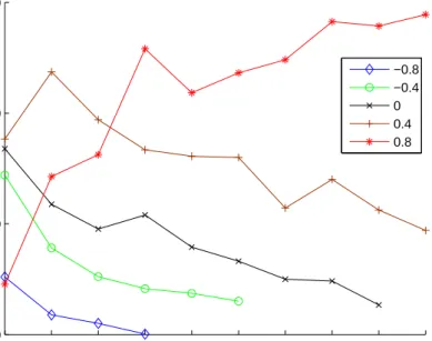
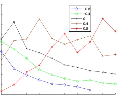
grid problems with ρ =0.8. Average values over ten random problems generated for each depth. . . 176 7.10 Space and time requirements forN AM OA∗∗ withH_KDLSk on class II

grid problems with ρ =0.4. Average values over ten random problems generated for each depth. . . 177 7.11 Space and time requirements forN AM OA∗∗ withH_KDLSk on class II

grid problems with ρ = 0. Average values over ten random problems generated for each depth. . . 178 7.12 Space and time requirements forN AM OA∗∗ withH_KDLSk on class II

(22)

7.13 Space and time requirements forN AM OA∗∗ withH_KDLSk on class II grid problems with ρ =-0.8. Average values over ten random problems generated for each depth. . . 180 7.14 Space requirements forN AM OA∗∗ withH_KDLSk inN Y2map. Problem

instances are ordered by increasing number of stored cost vectors needed

by N AM OA∗∗ with heuristicH_KDLS∞ . . . 182

7.15 Time requirements forN AM OA∗∗ withH_KDLSk inN Y2 map. Problem instances are ordered by increasing time needed by N AM OA∗∗ with heuristicH0

KDLS . . . 183 7.16 Class II grid problems with ρ =0.8. Average values over ten problems

generated for each depth. (a) Space requirements for N AM OA∗∗ with

H_KDLSk relative to graph solution size. (b) Time requirements for

N AM OA∗∗ withH_KDLSk relative to N AM OA∗∗ withH_KDLS0 . . . 185

7.17 Class II grid problems with ρ =0.4. Average values over ten problems generated for each depth. (a) Space requirements for N AM OA∗∗ with

7.18 Class II grid problems with ρ =0. Average values over ten problems generated for each depth. (a) Space requirements for N AM OA∗∗ with

7.19 Class II grid problems with ρ =-0.4. Average values over ten problems generated for each depth. (a) Space requirements for N AM OA∗∗ with

7.20 Class II grid problems with ρ =-0.8. Average values over ten problems generated for each depth. (a) Space requirements for N AM OA∗∗ with

Hk

KDLS relative to graph solution size. (b) Time requirements for

7.21 Ratiorv_ksol of space requirements forN AM OA∗∗ inN Y2 map, relative to solution graph size. Problem instances are ordered by increasing size of solution graph. . . 190 7.22 Time requirements for heuristics precalculation withKDLS procedure

on class II grid problems with ρ= 0. Average values over ten problems generated for each depth. . . 192 7.23 Ratio rt0_k of time requirements for N AM OA∗∗ with H_KDLSk in N Y2

map, relative to time requirements forN AM OA∗∗ with~hT C . . . 193 7.24 Time requirements for the multiobjective search phase ofN AM OA∗∗ with

H_KDLSk in class II grid problems withρ= 0 . . . 194 7.25 Number of label expansions ofN AM OA∗∗ usingHKDLS heuristics on

a sample200×200class II grid problem instance withρ= 0. Start node is (100,100) and goal node is (50,50). . . 196 7.26 Heuristic vectors obtained for start node (100,100) by KDLS on a

(23)

List of Figures xxiii

7.27 Number of vectors inH(n)andF(n)forN AM OA∗∗ usingHKDLS heuris-tics on a sample 200×200 class II grid problem instance with ρ = 0. Start node is (100,100) and goal node is (50,50). . . 199 7.28 Time to find the first solution forN AM OA∗∗ withH_KDLSk in class II

(24)

(25)

List of Tables

2.1 The N AM OA∗ algorithm. . . 29

2.2 The M OA∗ algorithm. . . 31 2.3 The T C algorithm. . . 33

3.1 Correlation between pairs of objectives for random graphs problems. . . 52 3.2 Road networks from DIMACS challenge (time/distance). . . 54 3.3 Road network from DIMACS challenge with modified objectives

(time/e-conomic cost). . . 54 3.4 Speed limits and fuel efficiency values associated to each road type. . . . 55 3.5 Modified Road networks from Tiger/Line Files of DIMACS challenge. . 56 3.6 Road networks for hazmat problems. . . 58

4.1 Trace of uninformed M OA∗ for the MC(2) graph. Contents of the OPEN list are displayed for each iteration. . . 73 4.2 Sets of heuristic cost values returned by heuristic functionH(n) =H∗(n)

for all nodes in graph MC(2). . . 73 4.3 Sample run of heuristic M OA∗ withH(n) =H∗(n) for MC(2) graph.

Contents of the OPEN list are displayed for each iteration. The lexico-graphic optimum amongF(n)values responsible for selection is underlined. 74 5.1 Estimated parameter values for the modelrp=α∗sβ and indicators in

the statistical analysis of the relative performance betweenM OA∗ and

N AM OA∗ on class I/II grid problems with different correlation values

(blind search) . . . 87 5.2 Summary of results from the empirical analyses on the performance of

N AM OA∗,M OA∗ and T C. . . 104

5.3 Algorithms evaluated in the empirical analyses performed on chapter 5. 119 5.4 Average heuristics precalculation time (in seconds) for modified DIMACS

road networks. . . 125

6.1 Number of road map problem instances that could not be solved in 1h

by N AM OA∗ with lexicographic selection . . . 140

6.2 Number of successful executions for road map problem instances that ex-ceeded at least once, but not always, the time limit withN AM OA∗ and lexicographic selection . . . 140

(26)

6.3 Data from NY map problems . . . 141 6.4 Data from BAY map problems . . . 142 6.5 Data from COL map problems . . . 143 6.6 Data from FLA map problems . . . 144 6.7 Speedup of heuristicN AM OA∗ with lexicographic selection with respect

to N AM OA∗ with~h₀ . . . 145

6.8 Speedup of heuristicN AM OA∗ with lexicographic selection and heuris-tic~h_{T C} with respect to~h_cd . . . 146 6.9 Run time (in seconds) for problem instances run without time limit with

N AM OA∗ and bounded~h_{T C} . . . 148

6.10 Algorithms evaluated for road map problem instances with time vs. eco-nomic cost (N Y2 map). . . 150 6.11 Data from NY₂ map problems . . . 152 6.12 Number of instances fromN Y2 map not solved in 12h . . . 152 6.13 Time requirements for heuristicNAMOA-LIN onN Y2problem instances

run without time limit . . . 153 6.14 Average speedup of heuristicN AM OA∗ overT C and blindN AM OA∗ for

N Y2 problem instances solved within runtime limit . . . 153 6.15 Average results on random graphs with 3 objectives for blind and

heuris-tic search withN AM OA∗ . . . 155 6.16 Average results on random graphs with objectives 1,2 for blind and

heuristic search with N AM OA∗ . . . 156 6.17 Average results on random graphs with objectives 1,3 for blind and

heuristic search with N AM OA∗ . . . 156 6.18 Average results on random graphs with objectives 2,3 for blind and

heuristic search with N AM OA∗ . . . 156 6.19 Average results on Lazio map for blind and heuristic search withN AM OA∗157

7.1 Precalculation of HKDLS for bicriteria search by KDLS procedure. . . 167 7.2 Sample graph for KDLS procedure: sets of stored supported solutions

and heuristic valuesH_KDLS∞ returned . . . 172 7.3 Analysis of dominance checks on a sample200×200class II grid problem

instance with ρ= 0. Start node is (100,100) and goal node is (50,50). . . 195 7.4 Size of C∗ set and number of heuristic vectors obtained for start node

(27)

Part I

Motivation and Fundamentals

This part introduces the motivation, goals, and contributions of this thesis. The fun-damentals of multiobjective graph search are presented, and previous relevant works are described in detail. In particular, the three algorithms analyzed in this thesis

(N AM OA∗, M OA∗ and T C) are described using a common framework. A review

of previous benchmarks on multiobjective search is conducted, and a set of relevant problem classes and instances are identified for the empirical analysis performed in subsequent chapters.

• Chapter 1 gives an overview of the contents, goals and contributions of this thesis.

• Chapter 2 presents the problem and the algorithms that will be subject of ana-lysis.

(28)

(29)

Chapter 1

Introduction

The context of this thesis is a common problem in the fields of Artificial Intelligence (AI) and Operational Research (OR). Shortest Path Problems appear in many everyday life situations, e.g. in car navigation systems, which plan the optimal route between some source and a specified destination point. Most available algorithms to solve this problem usually optimize a single criterion. The development and analysis of multiobjective shortest path algorithms is a relatively less explored area. The goal of this thesis is to deepen our undertanding of the formal and empirical behaviour of available exact multiobjective shortest path algorithms, with particular attention to heuristic search techniques. We also seek to analyze the benefits of heuristic search and to improve the performance of existing methods.

Section 1.1 introduces the motivation of this work. Scope and orientation are pre-sented in section 1.2. The goals of this thesis are summarized in section 1.3. Contri-butions are summarized in section 1.4. Related publications derived from this research can be found in section 1.5. Finally, an outline of the structure of this thesis is presented in section 1.6.

1.1 Motivation and Significance

Artificial Intelligence (AI) is one of the main branches of Computer Science (CS). Since the establishment of AI as a formal discipline, many of the most difficult problems in CS have been its subject of study. One recurrent problem in the AI literature is the Shortest Path Problem (SP). A minimal cost route between two points in a network can be obtained by algorithms like the one devised by Dijkstra (1959). Heuristic Search (HS) is an AI subdiscipline aiming to obtain more efficient algorithms, exploiting specific problem knowledge. An important reference is the A∗ algorithm (Hart et al., 1968), that uses cost estimates to guide search to the goal, improving efficiency.

Realistic decision problems frequently involve the consideration of multiple criteria at the same time. Figure 1.1 shows a sample scenario: planning a travel from Málaga to Lisbon seeking to minimize both time and economic cost. Among all feasible routes only a subset can be considered minimal in terms of both objectives. This is the so-called Pareto set. An alternative is Pareto-optimal if it cannot be improved in one objective without worsening some of the others, i.e. it represents an optimal tradeoff between the

(30)

(a) Best route concerning time (b) Best route concerning economic cost

Figure 1.1: Screenshots from a sample route planning application, showing alternative routes from Málaga to Lisbon.

objectives. The multiobjective search problem is known to be computationally more complex than single-objective search. Several methods and algorithms for this problem have been considered since the pioneering work of Hansen (1979).

In particular, several multiobjective heuristic search algorithms have been described in the literature, namely M OA∗ (Stewart & White, 1991), N AM OA∗ (Mandow & Pérez de la Cruz, 2005) and T C (Tung & Chew, 1992) algorithms. However, their formal and empirical analysis is relatively unexplored when compared to analogous single-objective algorithms.

Recent formal analyses have begun to clarify the benefits of heuristic information in multiobjective search (Mandow & Pérez de la Cruz, 2010a). However, little expe-rimental evaluation has been performed prior to this thesis to systematically compare the performance of multiobjective heuristic search algorithms.

The main goal of this thesis is to deepen our understanding of the performance of these algorithms. Research has been directed to complete formal analysis where needed, and to evaluate empirically the performance of heuristic search in general and realistic situations. In particular, the advantages of precalculated heuristics in multiobjective search are analyzed, and improved methods for heuristic precalculation are provided. The results obtained can be a useful guide for practitioners, and also point out clear lines of future research.

(31)

1.2. Scope and Orientation 5

generated problems provide an important testbed to control problem parameters, like solution depth or correlation between objectives. On the other hand, this thesis focuses on realistic route planning scenarios. These have been the subject of considerable research in the past few years for single-objective problems (Geisberger et al., 2008; Bast et al., 2007; Bauer & Delling, 2009; Goldberg & Harrelson, 2005), and emerge as an important potential area of application of multiobjective search.

1.2 Scope and Orientation

The boundaries of this doctoral dissertation are defined by the following terms:

Shortest path problems Problem instances involve the determination of shortest paths in graphs.

Additive costs Arcs are labelled with costs representing magnitudes to be minimized. The cost of a route between two nodes in a graph in terms of some magnitude can be obtained adding the corresponding magnitude costs of all arcs in the path.

Multicriteria scenarios Vector costs are considered in order to handle multiple ob-jectives at the same time. In general, practical analyses consider two obob-jectives, except for some simple scenarios where three objectives were considered.

Pareto optimality The scalar concept of minimum is no longer valid when multiple criteria are considered. Solutions must satisfy that no other feasible alternative can improve according to one objective whithout worsening at least one of the others.

Best-first exact algorithms All the algorithms and heuristics evaluated aim at the determination of the full Pareto-optimal set of solutions. Only best-first heuristic search is considered.

Empirical approach The research was guided mainly by practical experimentation with multiobjective heuristics and algorithms. Nevertheless, some theoretical results have been developed when necessary in order to explain the observed behaviour of algorithms, or complete previous formal analyses.

(32)

1.3 Research Goals

The main goals of this thesis can be summarized as follows:

Theoretical formalization One of the goals of this thesis is to complete the for-mal analysis of the heuristic performance of M OA∗, following the recent formal developments achieved for N AM OA∗. Additionally, some fundamental charac-terization of the T C heuristics is provided.

Empirical evaluation A second goal is to perform a systematic comparison of al-gorithms in order to determine which one performs better according to various problem parameters, like solution depth or correlation between objectives. Addi-tionally, we evaluate the performance of multiobjective search in realistic route planning domains. In all cases, we seek a deep understanding of the causes of the observed behaviours.

Effectiveness of heuristic search A third goal is to establish under which condi-tions heuristic search can actually improve the performance of multiobjective best-first algorithms from a practical point of view.

Improvements on current techniques A final goal is to use the knowledge gained through the formal and empirical analysis to explore new ways to improve algo-rithm performance. Special attention is paid to certain alternatives in algoalgo-rithm implementation, like the order of selection of alternatives for exploration.

1.4 Contributions of this Thesis

The main contributions of this thesis can be summarized as follows:

Analysis of M OA∗ The thesis completes previous formal analyses of M OA∗. Pre-vious analyses were unable to establish clearly the importance of heuristic in-formedness in algorithm performance. We show that the number of label ex-pansions of M OA∗ can be much larger with heuristic search than with blind search. In fact, performance can become worse even with the use of more in-formed consistent heuristics. This phenomenon is formally related to the node selection strategy used by M OA∗. In addition, empirical results show that this situation can easily appear in practice. As a result, M OA∗ can be discarded in general as a suitable alternative for multiobjective heuristic search.

Analysis of T C A simple characterization is provided to show that the precalculated heuristic devised by Tung & Chew (1992) is consistent. This has been recently identified as an important formal property for multiobjective heuristic search (Mandow & Pérez de la Cruz, 2010a). Systematic empirical analyses show for the first time that this heuristic can improve considerably the performance of both

T C and N AM OA∗ over blind search. However, T C was found to perform

(33)

1.5. Related Publications 7

Analysis of N AM OA∗ The algorithmN AM OA∗ has been found the most effective approach in most situations. However, certain situations have been identified where heuristic search can represent an overhead in time performance. These are the cases where the reduction of the number of alternatives considered does not compensate for the time penalty of early solution determination inherent to heuristic search. More precisely, this can be traced to the number of domi-nance checks needed by the algorithm. Additionally, empirical evaluation sug-gests that a linear selection rule significantly improves the time performance of

N AM OA∗ when compared to a traditional lexicographic one.

Precalculated heuristics The original precalculation method proposed by Tung & Chew (1992) can be improved in several ways. The original method requires the calculation of a one-to-all single-objective search for each objective under consideration. We have shown how the formal properties of N AM OA∗ let us bound the nodes that will be visited by N AM OA∗. This eliminates the need to consider in the precalculation stage those that will never be reached in the multiobjective search stage.

The original precalculatedT C heuristic provides a single vector estimate for each node. N AM OA∗ accepts general heuristic functionsH(n) with multiple heuris-tic vector estimates. A new calculation method, called KDLS, is presented in this thesis. More informed, multiple vector, heuristic functions can be precalcu-lated byKDLS. The precision of the new heuristic is determined by a parameter

k. Larger values ofkresult in more informed heuristics, but at the same time, re-quire more precalculation effort. In general, better heuristics considerably reduce the space requirements of N AM OA∗. However, time requirements are steadily increased in random grids, and only the smallest values ofkare competitive with the original approach in this sense. Nevertheless, in route planning problems multivalued heuristics can offer savings in both space and time requirements for some instances.

Applications in realistic scenarios The application of N AM OA∗ with informed heuristics has been shown to be competitive with state-of-the-art approaches to multiobjective search. Several different testbeds have been considered for route planning in road maps, a potential application area. Combinations of objec-tives distance/time, and the more complex time/economic cost, have been solved exactly with available resources over large road maps.

1.5 Related Publications

Several of the contributions presented in this thesis have been already published in international peer-reviewed conferences and journals:

• Journals:

(34)

Machuca, E. & Mandow, L. (2012). Multiobjective heuristic search in road maps.

Expert Systems with Applications, 39, 6435–6445.

• Conferences:

Machuca, E., Mandow, L., & Pérez de la Cruz, J. L. (2009). An evaluation of heuristic functions for bicriterion shortest path problems. In L. Seabra Lopes, N. Lau, P. Mariano, & L. Rocha (Eds.),New Trends in Artificial Intelligence. Proceedings of EPIA’09(pp. 205–216).: Universidade de Aveiro, Portugal.

Machuca, E., Mandow, L., Pérez de la Cruz, J. L., & Ruiz-Sepúlveda, A. (2010). An empirical comparison of some multiobjective graph search algorithms. In R. Dillmann, J. Beyerer, U. D. Hanebeck, & T. Schultz (Eds.),Advances in Ar-tificial Intelligence (Proceedings of KI’2010, 33rd Annual German Conference on AI, Karlsruhe, Germany, September 21-24), volume 6359 of Lecture Notes in Computer Science(pp. 238–245). Springer.

Machuca, E. & Mandow, L. (2011). Multiobjective route planning with precal-culated heuristics. In L. Antunes, H. Pinto, R. Prada, & P. Trigo (Eds.),Proc. of the 15th Portuguese Conference on Artificial Intelligence (EPIA 2011)(pp. 98–107).

Machuca, E., Mandow, L., Pérez De La Cruz, J. L., & Iovanella, A. (2011). Heuris-tic multiobjective search for hazmat transportation problems. In J. Lozano, J. Gómez, & J. Moreno (Eds.),Advances in Artificial Intelligence (Proceedings of the 14th international conference on Advances in Artificial Intelligence: Spa-nish Association for Artificial Intelligence - CAEPIA’11), volume 7023 of Lec-ture Notes in Computer Science (pp. 243–252). Berlin, Heidelberg: Springer-Verlag.

• Doctoral Consortium:

Machuca, E. (2009). Heuristics in best-first algorithms for multiobjective short-est path problems. In Doctoral Consortium, XIII Conference of the Spanish Association for Artificial Intelligence (CAEPIA’09).

Machuca, E. (2011). An analysis of multiobjective search algorithms and heuris-tics. InDoctoral Consortium, Proceedings of 22nd International Joint Confe-rence on Artificial Intelligence (IJCAI’11), Barcelona, 15-22 July (pp. 2822– 2823).

1.6 Outline

(35)

1.6. Outline 9

the task of empirical evaluation of algorithms. A literature review of previous relevant multiobjective benchmarks is presented. Finally, the different kinds of benchmark problems used in the empirical evaluations of this thesis are described in detail.

The second part groups all contributions of this thesis. Formal properties of

M OA∗ and the T C heuristic are established in chapter 4. A class of problems is devised to show that the complexity of M OA∗ can become worse with perfectly in-formed heuristics when compared to blind search.

Chapter 5 performs a systematic evaluation and comparison ofN AM OA∗,M OA∗, and T C. In the first place, the use of heuristic information is evaluated against blind search. Then, pair comparisons between the heuristic algorithms are performed. Some previously unnoticed phenomena are properly analyzed and explained. Moreover, the empirical results of M OA∗ confirm the bad results expected from the theoretical analysis of chapter 4.

Chapter 6 exploits the result obtained in previous chapters to evaluate the per-formance of multiobjective search in the domain of route planning in road maps. A bounded procedure for the calculation of the T C heuristic is presented. General time/distance and time/economic cost problem instances are evaluated. Additionally, a set of hazardous material transportation problems is also considered.

Finally, chapter 7 explores the possibility of more informed precalculated heuristics, extending the precalculation process of the T C heuristic to multiple-vector heuristic estimates. The new heuristic is tested on a set of selected problem benchmarks.

(36)

(37)

Chapter 2

MultiObjective Graph Search:

Problems and Algorithms

This chapter introduces the main concepts that will be used throughout the rest of this thesis. A definition of single-objective search problems and a brief review of relevant search algorithms is presented in section 2.1. A description of the multiobjective short-est path problem and basic multiobjective concepts follows in section 2.2. A review of the relevant blind algorithmic approaches for multiobjective search can be found in section 2.3. The heuristic algorithms analyzed in this thesis are described in section 2.4. Some formal properties about them and the heuristic functions used through most of the chapters of this thesis are also presented in this section. This includes the con-sideration of inconsistent heuristics in some detail. Finally, a review of relevant related heuristic works and a summary on multiobjective algorithms and heuristics is located at the end of the chapter.

2.1 Single-objective search

2.1.1 The Shortest Path Problem

The shortest path problem is probably one of the most studied problems by the Artifi-cial Intelligence (AI) and Operational Research (OR) communities (Gallo & Pallottino, 1988; Cherkassky et al., 1996; Pearl, 1984). Many real problems can be modelled as finding the shortest path between two nodes in a graph. Let us see a formal description of the problem.

LetG be a locally finite labeled directed graph G= (N, A, c) with|N|nodes and

|A|arcs (n, n0) labeled with positive values~c(n, n0)∈_R, wheren, n0 ∈N.

Definition 2.1 A pathP in (N, A) is a sequencehn1, n2, . . . , nli, whereni ∈N,∀i∈ [1, l]and(nj, nj+1)∈A,∀j∈[1, l−1]. The set of all possible paths inG is denoted by

P.

Definition 2.2 The cost of a pathP is defined as the sum of the costs of its

(38)

nent arcs,

c(P) = X

(n,n0₎_∈_P

c(n, n0) (2.1)

Definition 2.3 Given a start nodes∈N and a set of goal nodesΓ⊆N, theShortest Path problem (SP) consists of finding the path P ∈ P in G with the minimum cost c(P) froms to a goal node γ ∈Γ.

2.1.2 Shortest path algorithms

Shortest path algorithms can be classified in terms of different parameters: best-first/depth-first, blind/heuristic or exact/approximate, among others. A complete de-scription and a classification of different strategies has been recently devised by Korf (2010).

Best-first searchis based in the principle of optimality stated by Bellman (1954). This principle applied to shortest path problems means that every optimal path must be composed by optimal subpaths. Thus, best-first algorithms achieve the optimal solution choosing at each step the best promising alternative. Whenever more than one path reaches the same node, the best one is preserved while the others are discarded or pruned. Best-first search is a general strategy for solving shortest path problems in graphs. The main drawback is that it can exhaust memory resources for many problems, as all promising alternatives must be kept in memory.

On the contrary, depth-first search(Korf, 1985) only considers the best next promising alternative, forgetting other feasible ones which can be in fact part of the optimal path. Thus, the algorithm must backtrack to find the least cost solution path. Depth-first search is generally applied when there are not enough space resources to solve the problem and is specially adequate for solving tree problems.

Among the huge variety of algorithms solving the Shortest Path Problem, this thesis deals with exact best-first search strategies for graphs. Dijkstra’s algorithm (Dijkstra, 1959) is the most known blind algorithm in this sense for single-objective shortest path problems. However, the reference algorithm for shortest paths in AI is theA∗ algorithm (Hart et al., 1968; Pearl, 1984) which can be seen as a generalization of Dijkstra’s algorithm that uses heuristic cost estimates of the distance to goal(s) to improve search efficiency. The term heuristic search is used by the AI community for techniques that exploit knowledge about the problem in order to accelerate the solution of tough combinatorial problems.

A∗ and Dijkstra-like algorithms work in a similar way: several feasible alternatives are evaluated at each step for theselectionof the most promising one, according to a characteristic evaluation function for each noden. Letg(n)denote the accrued cost of a path fromston, while the heuristic functionh(n)an estimated cost of a solution fromn

to a goal nodeγ. For blind labelling strategies like Dijkstra’s algorithm, the evaluation function is f(n) = g(n), as h(n) = 0. Heuristic algorithms like A∗ incorporate with

h(n) an estimate of the distance to a goal node, i.e. forA∗ the evaluation function is

f(n) =g(n) +h(n) for each node n.

(39)

2.1. Single-objective search 13

Definition 2.4 Alabelstands for the cost of a path found to a given node. In single-objective algorithms each node nis labeled with a single-valued label, that stands for the cost of the current best known path to n.

A reference to the ancestor(s) of the label can be included, in order to recover the solution path, once the algorithm finishes. At each step a label from some node n is selected for expansion, and all the possible extensions via outgoing arcs of node n

are generatedand compared with actual stored labels in successor nodes. The label stored for an adjacent node n0 is updated when the extension of the selected path through some outgoing arc of n represent a least cost path to the node n0. Labels of dominated paths reaching a given node are discarded or pruned by virtue of the optimality principle (Bellman, 1954).

When a best-first strategy is used, the expanded label becomes permanent as the least cost to the node has been found. Otherwise, this is not guaranteed until all nodes have been examined, as the label can be corrected by a new better one. The former are known aslabel-settingalgorithms (Dijkstra, 1959) and the later aslabel-correcting

(Zhan & Noon, 2000).

This iterative node labelling process is repeated until the stopping criterion is ful-filled. The optimal cost of the path can be found in the label of the goal node when this is selected for expansion and the actual optimal path can be recovered tracing back pointers to parents.

The labels still pending evaluation are typically stored in an OP EN queue. A distinct set of CLOSED nodes can be used to store already evaluated alternatives, in order to perform duplicate detection and recover the solution path. In Dijkstra’s algorithm, each time a label is expanded, as best-first search is used, the optimal shortest path distance from sto the node is found. In the case ofA∗, the label will be permanent and a node will not come back to OP EN queue under some assumptions related to the heuristic functionh(n).

2.1.2.1 Formal properties

Definition 2.5 Let h∗(n) be the actual optimal cost of a path from n to goal nodes γ ∈Γ. A heuristic function h(n) isoptimistic when

h(n)≤h∗(n) ∀n∈N (2.2)

Definition 2.6 Let k(n, n0) denote the cost of an optimal path in G from a noden to another node n0. A heuristic function h(n) isconsistent when

h(n) +k(n, n0)≤h(n0) ∀n, n0∈N (2.3)

Definition 2.7 Equivalently, a heuristic function h(n) is said to bemonotonewhen h(n) +c(n, n0)≤h(n0) ∀(n, n0)∈A (2.4)

Definition 2.8 A heuristic functionh1(n)is said to bemore informed than another

heuristic function h2(n) when both are optimistic and

(40)

There is a strong relationship between the properties ofh(n)and the efficiency and quality of results produced by A∗ (Pearl, 1984).

Property 2.1 (Admissibility) Whenh(n)is a lower bound (optimistic) the search is considered admissible, i.e. it is guaranteed to find an optimal solution if this solution exists. A∗ is admissible even on infinite graphs with some additional assumptions:

∀n∈N, h(n)≥0 (2.6)

∀(n, n0)∈A, c(n, n0)≥ >0

Property 2.2 (Efficiency) When ∀n∈N, h(n) = 0, A∗ is equivalent to Dijkstra’s algorithm. When h(n) is consistent or monotone, A∗ requires in the worst case O(|N|) iterations, storingO(|N|) nodes in memory. If the cost of the optimal solution is denoted byc∗ =k(s, γ),A∗ will always expand for sure all labels withf(n)< c∗. For those with f(n) =c∗, only those belonging to the returned optimal solution path will be necessarily expanded. Given an optimistic heuristic function, more actual suboptimal alternatives can be pushed out the search frontier f(n) = c∗ with more informed heuristics, i.e. bigger values of h(n), reducing search effort.

Property 2.3 (Optimality) When the heuristic function h(n) is monotone, the cost of a path found by the algorithm is known to be optimal and it is not necessary to reopen nodes (an expanded node will not come back toOP EN). Moreover,A∗ is proven to be optimal among the class of admissible best-first algorithms1 (Dechter & Pearl, 1985), both in the number of expanded nodes and in the number of necessary iterations to find the solution. This means, that any expansion performed by the A∗ algorithm must be also performed by another algorithm in this class to preserve admissibility. Otherwise, there is no guarantee to find the optimal solution in all cases.

2.1.3 Application to route planning

Applied research in single-objective shortest paths includes the search for optimal routes in real road networks with Dijkstra’s algorithm (Zhan & Noon, 1998), A∗ (Zeng & Church, 2009) or even bidirectional A∗ (Klunder & Post, 2006). Efficient speedup techniques have been recently devised for route planning in road maps (Schultes, 2008) or train timetables (Schulz et al., 2000; Schulz, 2005).

In general, speedup techniques exploit information gathered in previous extensive searches of the map. The challenge is to achieve fast shortest-path queries with practical preprocessing time and memory. Two main categories can be found:

• Hierarchical techniques exploit the structure of the problem to prune unimportant nodes (or arcs). The most fruitful hierarchical technique, namely contraction hierarchies, is based in node contraction (Geisberger et al., 2008): nodes are removed orcontracted from the graph in some order while the shortest paths are preserved with additional arcs calledshortcuts. However multilevel graphs (Schulz et al., 2002), routing based in transit-nodes (Bast et al., 2007) or customizable

1_{These are defined as the class of unidirectional search algorithms that begin on a start node}_s_and

(41)

2.2. MultiObjective Shortest Path Problems 15

route planning (Delling et al., 2011a) based in advanced partitioning techniques of the graph like PUNCH (Delling et al., 2011b), have been also catalogued among other speedup techniques as effective for an improvement in the preprocessing of the graph or the time devoted to a query.

• Goal directed techniquescompute distance bounds or make some preprocessing on arcs to exclude those arcs that do not belong to an optimal path. SHARC (Bauer & Delling, 2009) or ALT (Goldberg & Harrelson, 2005) belong to this category. While the former precomputesarc-flags, the later precalculates optimal distances to certainlandmarks to provide distance bounds using the triangle inequality.

Both approaches, hierarchical and goal directed can be combined. A good overview of the possibilities is described by Bauer et al. (2010b). Moreover, some of the vast quantity of recent speedup techniques have been extended to other scenarios, like mobile or dynamic routing (Sanders et al., 2008), time-dependent planning (Batz et al., 2009) or multicriteria route planning (Geisberger et al., 2010; Delling & Wagner, 2009) for example.

The actual performance of speedup techniques depends on some decisions, taking into account the structural properties of the particular problem instance, e.g. the de-cision on which node is to be contracted in contraction hierarchies. A recent work established that the optimal adjustment for every instance in many recent techniques (for example, the assignment of landmarks to a graph in the ALT technique) is NP-hard (Bauer et al., 2010a). In practice, these adjustments are frequently settled experimen-tally with heuristics. Besides, most of these techniques are based in bidirectional search, in order to reduce time requirements.

A complete review of the literature on these techniques is out of the scope of this thesis. Good overviews of this field can be found elsewhere (Schultes, 2008; Delling et al., 2009; Bauer et al., 2010b).

Limited experiments have been performed on multiobjective route planning (Geis-berger et al., 2010; Delling & Wagner, 2009). This will be used as one of the benchmark problems used in this thesis (see chapter 3).

2.2 MultiObjective Shortest Path Problems

(42)

f1

f2

A

E

B

C

D

S

Suupppp..NNoonnddoomm..

N

NoonnSSuupppp..NNoonnddoomm..

D

Doommiinnaatteedd

F

FF

G

GG

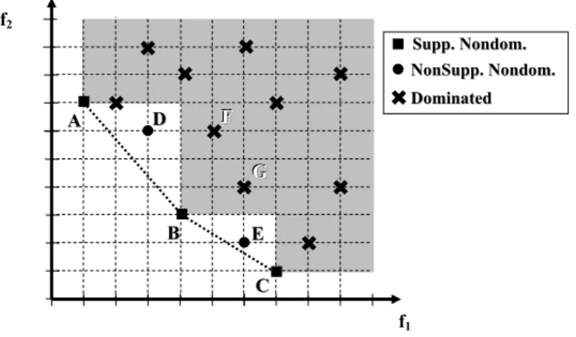
Figure 2.1: Supported, nonsupported and dominated points in a biobjective cost space

2.2.1 Basic Multiobjective Concepts

Multiobjective search algorithms differ from their scalar counterparts in several ways. First of all, the use of cost vectors in multiobjective problems induces only a partial order relation.

Definition 2.9 Let us consider two q-dimensional vectors~v, ~v0 ∈_Rq_{. A partial order}

relation ≺denominated dominance is defined as follows,

∀~v, ~v0 ∈_Rq, ~v≺~v0 ⇔ ∀i(1≤ i≤ q), vi ≤ vi0∧ ~v6=~v

0

(2.7)

where vi denotes the i-th component of vector ~v. Likewise, the symbol denotes the

relation “dominates or equals”.

Now, given two q-dimensional vectors ~v and ~v0 (where q > 1), it is not always possible to say that one is better than the another. For example in a bidimensional cost space (see figure 2.1) a vector (4,3)(point B) dominates (5,6) and (6,4) (points

F and G), but no dominance relation exists between (4,3)and (1,7)or (7,1) (points

A and C). They are said to benondominated.

Definition 2.10 Given a set of vectors X, we shall define nd(X) as theset of non-dominated vectors in X, i. e.,

nd(X) ={~x∈X |_@~y ∈X, ~y≺~x} (2.8) In the example of figure 2.1 the setndis{(1,7),(4,3),(7,1)}. Sometimes it becomes necessary to choose among nondominated vectors. Total orders can be defined in order to rank vectors.

Definition 2.11 Let us consider two q-dimensional vectors ~v, ~v0 ∈ _Rq_{. A total order}

relation ≺_lex denominated lexicographic order is defined as follows,

~v≺_lex~v0 ⇔ ∃j (1≤ j ≤ q), vj < vj0 ∧ ∀i < j, vi=vi0 (2.9)

(43)

Definition 2.12 Let us consider two q-dimensional vectors ~v, ~v0 ∈ _Rq_{. A total order}

relation ≺_lin denominated linear order is defined as follows,

~v≺_lin~v0 ⇔ X

i

vi <

X

i

v_i0 , 1 ≤ i ≤ q (2.10)

where vi denotes the i-th component of vector~v.

Definition 2.13 Let us consider two q-dimensional vectors ~v, ~v0 ∈ Rq. A total order relation ≺_wlin denominated weighted linear order is defined as follows,

~

v≺wlin~v0 ⇔

X

i

λivi <

X

i

λiv0i , 1 ≤ i ≤ q (2.11)

where vi, λi denote the i-th component of vectors~v, ~λ.

A useful property of the lexicographic, linear or weighted linear order is that their optimum in a set of vectors is also a nondominated vector. The order relations defined by ≺_lex,≺_lin or≺_wlin are total orders. Now, given twoq-dimensional vectors~vand~v0

(where q >1), it is possible to say that one is better than the another. For example, in a bidimensional cost space no dominance relation exists between (2,3) and (4,2). However,(2,3)≺_lex(4,2)and(2,3)≺_lin(4,2)(as2 + 3<4 + 2). Note that a derived total order can not always rank among two q-dimensional vectors, e.g. we can not say that (2,3)≺_wlin (4,2)for λ= (1,2) (as2∗1 + 3∗2 = 4∗1 + 2∗2). Some additional tie-breaking rule must be used.

Definition 2.14 LetX be the set of feasible solutions to a problem and letfk_:_X _→

R be k functions assigning a real value as image to a solution inX, being k= 1,2, . . . , q. A multiobjective problem in X can be formulated as a minimization problem,

minf~(x) = (f1(x), f2(x), . . . , fq(x)) (2.12)

s.t. ~x∈X

The criteria to be minimized2 _{at the same time (called} _objectives_{) are usually} conflicting so that there does not exist ~x ∈X optimal for the q dimensions. Thus, a multiobjective problem has in general more than onenondominated solution, rather than a single optimal solution. These are also called Pareto-optimal or efficient solutions in the literature

LetXE be the set of efficient or Pareto-optimal solutions to the minimization pro-blem of (2.12), and FE the set of nondominated image values on the objective space. Among the set XE, we can distinguish two different kinds of nondominated solutions:

Supported These ones can be obtained as optimal solutions to a single-objective weighted sum problem (WSP). For instance, for the biobjective case (i.e. q= 2), where~x= (x1, x2)

min

x∈Xλ1x1+λ2x2 (2.13)

2_{Note that there is no loss of generality considering minimization as the maximization case can be}

(44)

for some ~λ= (λ1, λ2). The set of all supported solutions can be denoted byXS, and the set of nondominated image values by FS. For example, see figure 2.1, where a sample bidimensional image space is depicted. Points A = (1,7), B = (4,3)and C = (7,1)represent supported solutions. The extreme nondominated solutions are supported solutions that have the minimum possible value in at least one of the objectives (points Aand C).

Non-Supported All the Pareto-optimal solutions in a continuous linear spaceRq are

supported. However, there can be remaining solutions, when dealing with discrete spaces (see figure 2.1). These remaining solutions in XN S = XE\XS are called

non-supported solutions as they cannot be obtained with linear combinations (WSPs). When solving a WSP, another supported solution will be found first, regardless of the slope used (i.e. regardless of the value of~λ). These solutions are located in the interior of triangles formed by two adjacent supported solutions, as depicted in figure 2.1. These areas are denominated by some authors as duality gaps (see the thesis of Raith (2009) for further details). The set of nondominated image values of XN S is denoted by FN S. These image values (points A, B and

C) dominate shaded areas in the figure, but not points D= (3,6)or E = (6,2).

Definition 2.15 Two feasible solutions ~x and ~x0 are called equivalent, denoted by ~

x=≺~x0, if their image values are the same, i.e. f~(~x) =f~(~x0).

Definition 2.16 Acomplete set XC ⊆XE is a set of nondominated solutions whose

image values, denoted by FC form the minimal set of distinct nondominated f~ values,

such that

∀~x∈X\X_E, ~x /∈nd(X) ∨ ∃~x0∈XC, ~x=≺~x0 (2.14) For instance, the setXE ={~x1, ~x2, ~x3, ~x4}denotes the set ofall efficient or Pareto-optimal solutions to a multiobjective problem. The nondominated image set FE =

{(1,2),(2,1)} has only two different vector values. A complete set XC = {~x1, ~x2} could include all different nondominated image values as FC = FE. However, two additional equivalent solutions can be found in XE, with ~x1 =≺ x~3 and ~x2 =≺ ~x4. A different set XN C = {~x1, ~x3} with nondominated image FN C = {(1,2)} would not include all nondominated solution values.

2.2.2 The Multiobjective Search Problem

Let G be a locally finite labeled directed graph G= (N, A, ~c) with|N|nodes and |A|

arcs (n, n0) where n, n0 ∈N, labeled with positive vectors~c(n, n0) ∈_Rq_{. The concept} of path in multiobjective problems remains the same as for single-objective case (see definition 2.1). However, the definition of the cost of a path for the multiobjective case must take into account that arcs are labelled with vectors.

Definition 2.17 The cost of a pathP in multiobjective problems is aq-dimensional vector C~P, and is defined as the sum of the costs of its arcs,

~

CP =~c(P) =

X

(n,n0₎_∈_P

(45)

n

nss

n

n33 nn44

n

ntt

n

n55 nn66 (5,4)

(1,2)

(2,1)

(2,7)

(1,2)

(3,5) (2,2) (3,1)

(1,2) (1,3)

(2,2)

(1,2)

n

n22 n

n11

Figure 2.2: A sample graph with some nondominated solution paths and equivalent solutions

Let P be the set of all possible paths in G. The set of all possible costs C~P of paths in

G will be denoted by _C_P.

Definition 2.18 Given a start node s∈N and a set of goal nodes Γ⊆N, let PsΓ be

the set of all pathsPsΓ ∈Pjoiningsand nodes inΓand letCsΓ be the set of all possible

costs C~sΓ ∈CP for paths inPsΓ. A multiobjective search problem (MSP) in Gconsists

of finding the set ofall nondominated pathsPE ∈PsΓ inGsuch that~c(PE)∈nd(CsΓ). This means that we are looking for efficient pathsPE inGsuch that

1. go from source node sto a node inΓ, i.e. PE ∈PsΓ

2. their cost is nondominated with other costs from paths in _P_sΓ

The Multiobjective Shortest Path Problem is also a minimization problem and can be formulated in a similar way to (2.12), 3

min~c(P) =~c(hn1, n2, . . . , nli) (2.17)

s.t. P ∈_P_sΓ

The Bicriterion Shortest Path Problem (BSP) is a particular case of MSP in which

q = 2, i. e., arc costs have two real components.

For graph search problems, the setXof feasible solutions to (2.13) isPsΓthe subset of paths in _P joining s and nodes in Γ the graph G, and the image function f~ to be minimized from (2.12) is the cost of each feasible path PsΓ ∈ PsΓ, i.e f~(x) =~c(PsΓ). For instance, see the path hns, n5, n6, nti from source node ns to goal nodent across

3

It was denominated by Hansen (1979) for the bicriteria case, where arcs are labelled with costs (c1(n, n0), c2(n, n0)), as MINSUM-MINSUM because it tries to find

min X

(n,n0_)∈P

c1(n, n0) ∧ min

X

(n,n0_)∈P