of graphs and tensegrities
Jose David Fernández RodríguezUniversidad de Málaga Málaga, Málaga (Spain) [email protected]
David Orden Martín Universidad de Alcalá Alcalá de Henares, Madrid (Spain)
Abstract
In this study, a complexity measure for graphs and tensegrities is proposed, based on the concept of atomic decomposition.We state several results on the relationship between atomic decompositions and spaces of self-stresses for generically rigid graphs, and study the computational complexity of finding atomic decompositions of minimal length.
1
Introduction
The concept of tensegrity is nowadays widely used in many disciplines, from biomechanics to structural engineering. Loosely speaking, a tensegrity is a structure whose elements are bound together in a stressed state, while the whole is in equilibrium. Over the years, each discipline has tailored the meaning of the word tensegrity to its own needs. Consequently, there are many definitions of tensegrity, each one subtly different from the others. We will stick to one of the simplest, broadest and more tractable definitions.
Up to date, it is usual to discuss about the complexity of tensegrity structures without trying to measure it, among other reasons because finding an agreeable complexity measure is problematic. Fur-thermore, existing complexity measures are usually too general to be useful in a specific context. In this work we propose a method to measure the complexity of tensegrity structures, taking into account their tensegrity nature.
Before starting our discussion, let us present here briefly the concepts and results (mostly) formulated in [11] that we need to present our work:
• A finitepoint configuration P:={p1, ...,pn}inRd is ingeneral positionif nod+1 points lie on
the same hyperplane. More restrictively, if the points are algebraically independent, the position is generic.
• A framework G(P) in Rd is an embedding of the abstract graph G= (V,E) on a finite point
configurationPinRdin general position, with straight edges.
• Aself-stress won a framework is an assignment of scalarswi j (called tensions) to its edges, such
that for each vertexi, the scaled sum of incident vectorspi−pjis zero:
∀i,
∑
i j∈E
wi j(pi−pj) =0
Observe that self-stresses form a vector space.
• If a frameworkG(P)hasnvertices andeedges, its associatedrigidity matrix R(P)haserows and ndcolumns, such that:
– There is a row per edgei jof the framework, withi< jand in lexicographic order.
– Each block ofd columns is associated to a vertex pi, and it contains zeros except for each
Observe that ifwis a self-stress onG(P), thenw·R(P) =0.
• A framework with a self-stress non-null on every edge is called atensegrity, denoted asG(P,w).
• An atom A in dimensiond is a complete graphKd+2 embedded in Rd. If the embedding is in
general position, its space of self-stresses has dimension 1. Otherwise, it only admits a null stress, that is to say,wi j=0,∀i,j.
• Anatomic decompositionof a tensegrityG(P,w)is a finite set of atoms (each atom corresponding
to a set ofd+2 points inP) such that the sum of their self-stresses isw. Note that the atoms in the decomposition may have edgesi jnot present inG, which cancel out towi j=0 when the atom
stresses are added up. In general, decompositions are not unique. Thelengthof the decomposition is the cardinality of the set of atoms.
One of the main results in [11] is the development of an algorithm to generate atomic decompositions for tensegrity structures. The algorithm can be applied to a tensegrityG(P,w)(Theorem 3.2 in [11]), or to an abstract graphG= (V,E)(Algorithm 3.4 in [11]). In this work, we will refer to these variants as the
geometricandcombinatorial algorithms, respectively. Below, the combinatorial version of the algorithm
is reproduced:
Algorithm 1.1. (Adapted from Algorithm 3.4 in [11])Atomic combinatorial decomposition
INPUT: abstract graph G= (V,E)and dimension d.
OUTPUT: (L,M,F), where L is a list of “atoms” (subsets of (d+2) elements of V ), M is a list
containing the number of edges added for each atom in L, and F is a list of intermediate graphs.
1. Initialize L=∅, M=∅, F= [G].
2. While E is not empty, choose a vertex a∈V and:
2.1 If a has degree d+1, let a0, . . . ,adbe its neighbors. Remove the edges aaifrom E. Let E0be
the set of all the edges aiajbetween the neighbours that were not in E.
2.2 If a has degree at least d+2, choose d+1neighbors a0, . . . ,ad of a. Remove the edge aa0
from E. Let E0be the set of all the edges aiaj between the neighbours that were not in E.
2.3 If a has degree≤d, remove its incident edges from E.
In cases 2.1 and 2.2, also add the edges from E0to E, insert the atom{a,a0, . . . ,ad}to the list L,
and|E0|to the list M. In any case, also update the graph with the new set of edges and removing
unconnected vertices, and add it to the list F.
3. Return(L,M,F).
It is important to note that both the geometric and the combinatorial algorithms are non-deterministic: different decompositions can be obtained by making different sets of choices at several points in the algorithms. In the combinatorial algorithm, the resulting decomposition of a graphGrepresents a set of constraints between the positions of vertices and/or self-stresses of edges of tensegrities with underlying graphG. More details in [11].
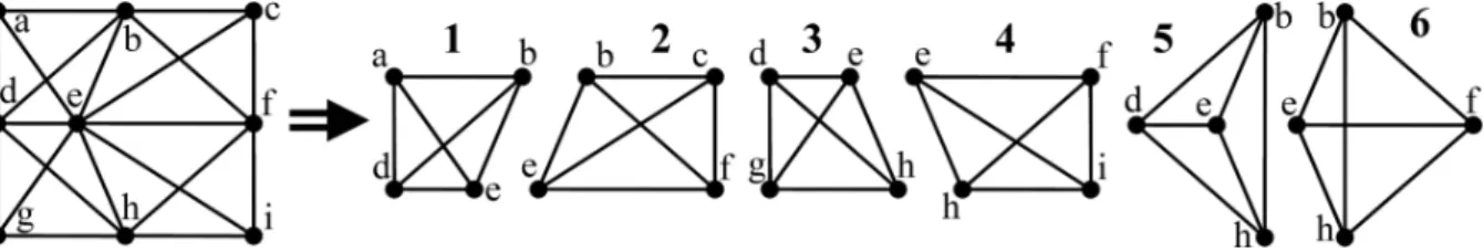
Figure 1: An abstract graph with one example of a combinatorial atomic decomposition.
Remark 1.2. While the combinatorial algorithm formally operates in the domain of abstract graphs, it implicitly assumes that the graph is embedded in some unspecified tensegrity. In this context, it is
significant to note that some valid tensegrities G(P,w)might have a SAL shorter than the combinatorial
SAL for G. Consider the decomposition shown in Figure 1: if we set a general point configuration P
and define a self-stress w which is the sum of atoms1, . . . ,4, we can obtain a tensegrity G(P,w)whose
underlying graph G is the same as the one depicted in the figure. Therefore, while the geometric SAL of
this specifically constructed G(P,w)is 4, the combinatorial SAL for G is 6, because the combinatorial
algorithm tacitly assumes that G is implicitly embedded in a tensegrity G(P,w)as generic as possible,
both in terms of the position P and of the self-stress w. However, as we will see in Section 2.2, the combinatorial problem can be reduced to the geometric one.
From rigidity theory [9], we know that the setW of all possible self-stresses of a frameworkG(P) is, in fact, the left kernel of the matrix R(P). Similarly, the space of infinitesimal motions is the right kernel ofR(P), whose dimension (or number of degrees of freedom) is 0 ifG(P)is rigid. The following proposition relates the dimensions of both spaces:
Proposition 1.3. (Theorem 2.4.1 in [9])Let G(P)be a framework in general position P in dimension d with G= (V,E),WG(P)
the dimension of the self-stress space anddf(G(P))the number of degrees of
freedom of G(P). Then:
df(G(P)) =
WG(P)
−
d+1
2
+d· |V| − |E|, if|V| ≥d
|V|
2
− |E|, if|V| ≤d+1
(1)
2
The structure of the space of self-stresses
For all practical purposes, we will be interested in graphs which are generically rigid, that is to say, rigid in any generic position. Non-generically rigid graphs can be tensegrities only in very degenerated positions. We will use|WG|to mean the dimension ofWG(P)ifPis a generic position, since it is constant
for every generic position.
For generically rigid graphs, the space of self-stresses of the intermediate graphs (list F) in the decomposition algorithm changes according to the number of intermediate edges inserted along the de-composition (listM), and these numbers are directly related to the dimension of the space of self-stresses. To show this, we start with the following proposition:
Proposition 2.1. If a graph G= (V,E)is generically rigid inRd, then every intermediate graph in any
Proof. Suppose that, for a given decomposition, the list of intermediate graphs isF= [. . . ,Gi,Gi+1. . . ,].
We can prove the proposition by showing that if an intermediate graphGiis generically rigid, thenGi+1
also is. We do it by cases:
• If the transition is done by step 2.1, let E0 be the set of the added edges fromGi toGi+1. IfGi
is generically rigid, consider the rigidity of the graphG0i+1, induced fromGi+1 by removing the
edges inE0. IfG0i+1 is not generically rigid, then the edges incident toa inGi must remove all
degrees of freedom fromG0i+1, which allows the movement of some of its neighbours relative to others. InGi+1, all distances between these neighbours are fixed by the edges added inE0, soGi+1
is also generically rigid.
• If the transition is done by step 2.2, letaa1be the only edge removed fromGi toGi+1. InGi+1,
the subgraph induced by the verticesa,a1, . . . ,ad is a cliqueKd+2minus an edge. A cliqueKd+2
is a generic rigidity circuit in dimensiond(Theorem 3.11.9.a in [9]). If an edge is removed from a rigidity circuit, the resulting subgraph is still generically rigid (in chapter 3 in [9]). Therefore, the relative positions ofaanda1are fixed inGi+1, and hence this is also generically rigid.
• If the transition is done by step 2.3, at mostdedges have been removed fromGitoGi+1. Reasoning
by the number of vertices inGi:
– if|Vi|>d, the vertexamust have exactlyd incident edges forGi to be rigid, and any
self-stress must be always zero in these edges. Therefore, the equilibrium at other vertices inGi
is independent from these edges, and|WG|remains the same inGiandGi+1. By applying the
first case of Equation 1, we get that df(Gi+1) =0, soGi+1is also generically rigid.
– if|Vi| ≤d,Gimust be a complete graph in order to be generically rigid by the second case of
Equation 1, soGi+1will also be a complete graph, hence also generically rigid.
Therefore, generic rigidity is a property conserved through all intermediate graphs in the decompo-sition algorithm. To take advantage of this, we define theLaman bound:
Definition 2.2. TheLaman boundof a generically rigid graph G= (V,E)in dimension d is defined as:
B=
d+1
2
−d· |V|+|E|
The Laman bound is modified by the decomposition algorithm in a very specific way:
Proposition 2.3. Let Gi,Gi+1be two successive intermediate graphs in a combinatorial atomic
decom-position in dimension d, with every vertex in Gihaving degree at least d. Let Biand Bi+1be their Laman
bounds, respectively, and let eibe the number of edges added from Gito Gi+1. Then, Bi+1=Bi+ei−1.
Proof. By the definition of Laman bound, it is easy to see that the equality holds in any case (steps 2.1,
2.2 and 2.3).
If a graph is generically rigid and has at leastdvertices, thenB=|WG|by Proposition 1.3. Hence,
by Proposition 2.1, each atom considered in the decomposition algorithm changes the dimension of the space of self-stresses of the intermediate graph, according to the number of edges added to the graph. Atoms adding no edges represent an independent dimension inWG, atoms adding one edge must be tuned
to cancel out the stress in that edge, so they do not affect the dimension ofWG, and atoms adding two or
Proposition 2.4. Let G be a generically rigid graph and B its Laman bound, and consider the lists L (of
atoms) and M=
e1,. . . ,e|L|
(of amounts of added edges) produced by an atomic decomposition of G. Then, the number of atoms in the decomposition is the Laman bound plus the total amount of (possibly repeated) edges added during the decomposition:
|L|=B+ |L|
∑
i=1
ei (2)
Proof. AsGis generically rigid, Proposition 2.3 can be applied to every intermediate graph generated
by the algorithm, so an atom introducingeedges changesBbye−1. Equality 2 is implied by combining Proposition 2.3 with the fact that the Laman bound must change fromB0=BtoB|L|=0.
The previous proposition provides a characterization of the SAL: it corresponds to the decomposi-tions introducing the fewest edges in the intermediate steps. This holds even if the graph is not generically rigid.
Definition 2.5. A decomposition is defined asatomisticit no edges are added in any intermediate step.
By extension, a graph isatomisticif it admits an atomistic decomposition.
It is clear that, in an atomistic decomposition, the self-stresses of the atoms form a basis forWG.
It is also evident that if a graphG= (V,E) is decomposed andE0 is the set of all edges added in the intermediate steps, then the graphG0= (V,E∪E0)is atomistic. Also, chordal graphs that are generically rigid are also atomistic, and so are cliquesKn, whose minimal decomposition length is n−2d
. 2.1 Tensegrity complexity revisited
At first glance, it seems natural to define the complexity of a tensegrity as the smallest|L|over all the possible outputs of Algorithm 1.1. Then, cliques would be maximally complex under this definition and, in general, very dense graphs would tend to have relatively large SALs. However, we can use the relationship between atomic decompositions and the structure of the generic self-stress spaceWG of a
graphG, in order to get a more descriptive definition. Since each edge added during the decomposition represents an interlock between the self-stresses of several atoms, the more edges, the more complex must be the interlock between the self-stresses of the atoms in the decomposition, in order to form the desired tensegrity. Thus, the number of edges added during the decomposition seems to be a better measure of the complexity of a tensegrity, bearing in mind that it should be used to compare graphs with the same or nearly similar number of vertices.
2.2 An algebraic characterization
Given a tensegrityG(P,w), the geometric decomposition algorithm (check the combinatorial version in Algorithm 1.1 or the geometric version in [11]) admits an algebraic reformulation.
Remark 2.6. Note that we are moving from combinatorics to geometry now. Most of the (combinato-rial) graphs we are interested in can be realized as a (geometric) tensegrity although, as described in
Remark 1.2, some valid tensegrities G(P,w)might have a SAL shorter than the combinatorial SAL for
G. If a generically rigid graph G= (V,E)can be a tensegrity, the way to find P and w to construct a
tensegrity G(P,w)depends on the value of|WG|:
• If|WG|>0, and no edge in E must have a null self-stress for a generic position P, any generic
P will be suited to construct a tensegrity G(P,w). Given a generic P (uniformly random
taking a basis{w1, . . . ,wk}for WG(P), and finding a linear combination w=∑aiwi where
coeffi-cients ai are drawn from a uniform distribution U(0,1).
• If|WG|=0and a tensegrity G(P,w), can be defined, then the configuration P must be non-generic.
In some cases, it can be found relatively easily (for example, for graphs with edge-inserting de-compositions, as described in [11]).
Definition 2.7. Let P be a point configuration in dimension d. We define Qmas the collection of all sets
with exactly m vertices from P. We also define theatomic self-stresses matrix, named S, as follows:
• There is a row for each possible setpi,pj ∈Q2. The rows are ordered by the indices i,j, with
i< j and in lexicographic order.
• There is a column for each possible set{p1, . . . ,pd+2} ∈Qd+2. As these d+2points represent an
atom A, let wA be an unitary, non-null self-stress of A. Then, the column associated to A contains,
for each row corresponding to a pair of points pi,pjof A, the self-stress assigned by wAto the edge
pipj. In every other row, the value is 0. As with the rows, the columns are ordered in lexicographic
order by the indices of the points.
For a given tensegrity G(P,w), the self-stress w can be represented as a column vector w of length
n d+2
, where there is a position for each possible pair pi,pjof vertices of the framework, with i< j and
in lexicographic order, and the value in w for the position corresponding to the pair pi,pj is wi j if there
is an edge between them, and 0 otherwise.
It is easy to see that ifwis a valid self-stress ofG(P), then every solutionxto the underdetermined system of linear equations S·x=w represents a linear combination of atoms which can be used to construct a tensegrityG(P,w). Furthermore, letkxk0be number of non-zero elements inx. The problem of finding the SAL can be recast as finding a sparsest solution (with minimalkxk0) toS·x=w. Since by Remark 2.6 the combinatorial algorithm can be restated in these terms for most graphs, this leads to some interesting properties forS:
Corollary 2.8. If a configuration P in n vertices is in general position, the rank of the corresponding atomic self-stresses matrix S is n−2d.
Proof. Knis an atomistic graph, so any SAL minimal decomposition corresponds to a basis forWKn. As
the columns of the matrixSare the self-stresses for all possible atoms inKn, its rank must be exactly the
size of this basis, i.e., n−2d.
It is interesting to consider how Proposition 2.4 translates into this algebraic setting. First, we need some definitions:
Definition 2.9. Let G(P) be a framework, and Q2,Qd+2 as in Definition 2.7. Given a set of pairs
D⊆Q2, we define its collection of associated atomsAD⊆Qd+2 as the collection of all sets of d+2
points including some member of D, i.e., AD=
. . . ,pi, . . . ,pj, . . . ∈Qd+2|
pi,pj ∈D .
Definition 2.10. Let G(P,w) be a tensegrity, with G= (V,E) its underlying graph, S its atomic
self-stresses matrix and w the column vector associated to w, as in Definition 2.7. Let E0 ⊆Q2 be a set
of edges containing E. Let G0 = (V,E0) be a graph formed by adding the edges in E0−E to G. Let
AE0⊆Qd+2be the set of atoms associated to E0. The rows (resp. columns) of S correspond one-to-one to
sets in Q2(resp. Qd+2). We define thecoreof S (resp. w) with respect to E0, denoted SE0 (resp. wE0), as a
the submatrix of S (resp. w) induced by E0, whose rows correspond to E0and whose columns correspond
Now, it is worth to note that any solution xE0 toSE0·xE0 =wE0 induces a solutionx (generated by
padding xE0 with zeros for the rows in S but not in SE0) to S·x=w (in fact, kxE0k
0 =kxk0). The
following insight relates the structure of a combinatorial decomposition to the solution to the linear system of equationsS·x=w:
Proposition 2.11. Let G(P,w)be a tensegrity with graph G= (V,E), such that Proposition 2.4 holds (as
in Remark 2.6). Then, the SAL corresponds to a minimal set of edges Ea such that, for E0=E∪Ea, it
holds thatrank(SE0) =rank([SE0|wE0]), where SE0 and wE0 are the cores of S and w.
Proof. LetLbe any geometric decomposition ofG(P,w), letEabe the set of edges added during
decom-positionL, and letE0=E∪Ea.Lcan be recast as a solutionxE0 toSE0·xE0 =wE0. Then, Proposition 2.4
means thatkxE0k
0 is the sum of the dimension of the space of self-stresses ofG(P)and the number of
rows inSE0 corresponding to edges inEa. Therefore, a SAL will correspond to a minimal set of edgesEa
such that the systemSE0·xE0 =wE0 is solvable. The solvability condition can be restated in terms of the
ranks of the matrix and the augmented matrix, rank(SE0) =rank([SE0|wE0]).
As a result, atomistic graphs can be characterized in algebraic terms: if a suitable tensegrityG(P,w) is defined on a graph G= (V,E) (as in Remark 2.6), then it is atomistic if and only if rank(SE) =
rank([SE|wE]).
3
Computational complexity
The problem of computing the SAL seems to be NP-complete, but the question remains open. As the combinatorial atomic decomposition is defined through an algorithm with some non-deterministic steps, a choice (selected atom) taken in a step affects in highly convoluted ways to the choices available in all subsequent steps. Because of this, it is very difficult to reason directly about the computational complexity of finding the SAL. While several NP-complete problems seem to be very related to it, no obvious ways to reduce them to it have been devised:
The NP-completefixed clique covering problem(FCC) [12, 5] is (for any givenn) the problem of finding the minimal amount of copies of Kn needed to cover all the edges of a graphG, where these
copies are not required to be induced subgraphs ofG. FCC can be deemed as a non-trivial lower bound on the SAL in dimensiond, but, unfortunately, the FCC tends to grossly underestimate the SAL.
The NP-completeminimum fill-in(MFI) [18] of a graphGis the minimal amount of edges whose addition makes the graph chordal. If a graph can be instantiated as a tensegrity in dimensiond, its MFI plus its Laman bound can be regarded as an upper bound on its SAL, as the resulting chordal supergraph will necessarily have at least as many edges as a minimal atomistic supergraph ofG(in fact the chordal supergraph will induce an atomic decomposition ofG, although not necessarily minimal). As chordal graphs are also atomistic, the MFI induces a SAL in many cases. These facts hint that, even if the problem is not NP-complete, it must be relatively hard to solve.
is always extremely low (at most seven for dimensiond =2, since six vertices induce seven linearly dependent atoms). As a result, these methods yield very sub-optimal solutions to the SAL in most cases.
4
Acknowledgements
The present work was developed during a stay of Jose David Fernández Rodríguez at the Universidad de Alcalá, partially supported by the Departamento de Matemáticas de la Universidad de Alcalá. Jose David Fernández Rodríguez is partially supported by the Ministerio de Educación del Gobierno de España through a FPU grant (AP2007-03704). David Orden Martín is partially supported by grants MTM2008-04699-C03-02/MTM and MTM2011-22792. The second author wants to gratefully acknowledge fruitful discussions with Carlos Marijuan.
References
[1] A. Aspremont and L. El Ghaoui, Testing the nullspace property using semidefinite programming, Mathemat-ical Programming(2010), 1–22.
[2] A.M. Bruckstein, D.L. Donoho and M. Elad, From sparse solutions of systems of equations to sparse mod-elling of signals and images,SIAM Review51(2009), 34–81.
[3] E. Candès, M. Wakin and S. Boyd, Enhancing sparsity by reweighted L1 minimization,Journal of Fourier Analysis and Applications14(2008), 877–905.
[4] S.S. Chen, D.L. Donoho and M.A. Saunders, Atomic decomposition by basis pursuit, SIAM Review43 (2001), 129–159.
[5] D.G. Corneil and J. Fonlupt, The complexity of generalized clique covering,Discrete Applied Mathematics 22(1989), 109–118.
[6] D. Donoho, For most large underdetermined systems of linear equations the minimal L1-norm solution is also the sparsest solution,Communications on pure and applied mathematics59(2006), 797–829.
[7] S. Foucart and M.J. Lai, Sparsest solutions of underdetermined linear systems viaLq-minimization for 0<
q<=1,Applied and Computational Harmonic Analysis26(2009), 395–407.
[8] J.J. Fuchs, Sparsity and uniqueness for some specific under-determined linear systems, Proceedings of the IEEE International Conference on Acoustics, Speech, and Signal Processing(2005), v/729 - v/732 Vol. 5. [9] J.E. Graver, B. Servatius and H. Servatius,Combinatorial Rigidity, Graduate Studies in Mathematics, Vol. 2,
American Mathematical Society, 1993.
[10] R. Gribonval and M. Nielsen, Sparse representations in unions of bases,IEEE Transactions on Information Theory49(2003), 3320–3325.
[11] M. Guzman and D. Orden, From graphs to tensegrity structures: geometric and symbolic approaches, Publi-cacions Matematiques50(2006), 279–299.
[12] L.T. Kou, L.J. Stockmeyer and C.K. Wong, Covering edges by cliques with regard to keyword conflicts and intersection graphs,Communications of the ACM21(1978), 135–139.
[13] M. Lai, On sparse solutions of underdetermined linear systems,Journal of Concrete and Applicable Mathe-matics8(2010), 296–327.
[14] Y. Li and S.I. Amari, Two conditions for equivalence of 0-norm solution and 1-norm solution in sparse representation,IEEE Transactions On Neural Networks21(2010), 1189–1196.
[15] D. Malioutov, M. Cetin and A. Willsky, Optimal sparse representations in general overcomplete bases, Pro-ceedings of the IEEE International Conference on Acoustics, Speech, and Signal Processing(2004), ii - 793-6 vol.2.
[16] B.K. Natarajan, Sparse approximate solutions to linear systems, SIAM Journal on Computing24 (1995), 227–234.
[17] Y. Tsaig and D.L. Donoho, Breakdown of equivalence between the minimalL1-norm solution and the sparsest