PROGRAMA DE DOCTORADO EN MATEMÁTICAS
TESIS DOCTORAL:
TRIMMING METHODS FOR MODEL
VALIDATION AND SUPERVISED
CLASSIFICATION IN THE PRESENCE OF
CONTAMINATION
Presentada por Marina Agulló Antolín para optar al
grado de
Doctora por la Universidad de Valladolid
Dirigida por:
iii
Agradecimientos
En primer lugar, quiero agradecer a Tasio el haberme dado la oportunidad de realizar este trabajo con ´el, todo el tiempo y el trabajo que me has dedicado y lo mucho que me has ense˜nado a lo largo de estos a˜nos. Tambi´en quiero agradecer a Carlos todo lo que me ense˜naste en los primeros pasos de esta tesis. No quiero olvidarme de Jean-Michel, gracias por la acogida que me diste cuando llegu´e a Toulouse, por todo el tiempo que me has dedicado y por el inter´es que siempre has mostrado en mi trabajo. Quiero agradecer a todo el departamento de Estad´ıstica e Investigaci´on Operativa lo bien que me han tratado a lo largo de estos a˜nos, en especial quiero agradecer a Jes´us Saez toda la ayuda que me has dado.
Tambi´en quiero agradecer a todos y cada uno de los maestros y profesores que he tenido a lo largo de mi vida, porque todos han puesto su granito de arena en mi formaci´on. En especial a mi profesor de matem´aticas del instituto que fue el que me meti´o dentro el gusanillo de las matem´aticas y siempre insisti´o en que deb´ıa olvidarme de la psicolog´ıa y estudiar matem´aticas.
Quiero agradecer tambi´en a todos mis compa˜neros de viaje, todas esas doctorandas y doctorandos que hab´eis compartido estos a˜nos conmigo. No os nombro a todos porque sois muchos, pero vosotros sab´eis quienes sois, los matem´aticos (de la UVa y de fuera) y tambi´en los f´ısicos. Muchas gracias por vuestra amistad, por vuestro apoyo en los momentos dif´ıciles y por compartir mi alegr´ıa en los buenos. Aunque algunos haya sido en la distancia siempre hab´eis estado ah´ı. Voy a echar mucho de menos nuestras comidas y nuestras patatas de los jueves. Gracias a todas las personas que hab´eis hecho que adaptarme a una ciudad nueva no haya sido tan dif´ıcil, en especial gracias a Carmen y familia por haber tenido siempre un hueco para mi en vuestra casa, gracias a mis tios y primos y gracias a las dos alicantinas con las que he tenido la suerte de coincidir aqu´ı. Gracias a todos mis amigos de Elche (y alrededores) que siempre hab´eis estado a mi lado a pesar de la distancia, por haber tenido siempre un rato para mi cuando iba de visita y por haber estado siempre al tel´efono cuando lo he necesitado. Gracias a Tamara y a Patri por esa amistad eterna, no recuerdo mi vida sin vosotras a mi lado y espero no tener que hacerlo nunca.
Contents
1 Introduction 1
1.1 Introducci´on en Espa˜nol . . . 1
1.2 Introduction in English . . . 8
2 Preliminaries 15 2.1 Statistical methods based on trimming . . . 15
2.2 The classic classification problem . . . 18
2.2.1 Vapnik-Chervonenkis theory. . . 22
2.2.2 Loss functions, SVM and LASSO . . . 23
2.3 Optimal transportation problem and Wasserstein metrics . . . 25
2.4 Deformation models. Alignment . . . 27
2.5 Algorithms . . . 28
2.5.1 Optimal transportation algorithms . . . 30
2.5.2 Gradient methods . . . 38
2.5.3 Concentration algorithms . . . 40
3 Partial transportation problem 43 3.1 Trimming and Wasserstein metrics . . . 44
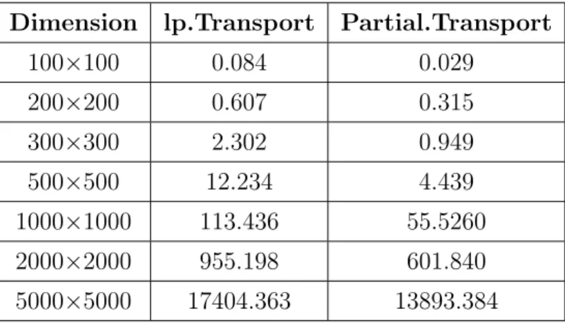
3.2 The discrete partial transportation problem . . . 46
3.2.1 A fast algorithm for the partial transportation problem . . . 52
3.3 Stochastic approximation for computation of o.t.c. . . 56
3.4 Application to contaminated model validation . . . 67
3.5 Algorithm and simulations. . . 78
vi Contents
4 Deformation models 83
4.1 A model for distribution deformation . . . 84
4.2 Estimation of the warping parameters . . . 85
4.3 Computational aspects . . . 91
4.4 Examples . . . 92
4.5 Simulations . . . 94
5 Partial classification problems 103 5.1 Problem statement . . . 104
5.2 Partial Classification with 0/1 loss . . . 105
5.2.1 Optimal trimming level selection . . . 117
5.3 Partial SVM classification . . . 130
5.3.1 Optimal trimming selection . . . 137
5.3.2 Algorithm . . . 149
5.3.3 Simulations . . . 151
5.3.4 Example with real data . . . 158
5.4 Extensions. . . 159
5.4.1 Penalization based on Kullback’s divergence . . . 160
5.4.2 Penalization based on Wasserstein distance . . . 165
5.4.3 Other loss functions . . . 169
6 Conclusions and future work 173 6.1 Conclusiones y trabajo futuro . . . 173
6.2 Conclusions and future work . . . 176
Chapter
1
Introduction
1.1
Introducci´
on en Espa˜
nol
La debilidad de muchos procedimientos estad´ısticos cl´asicos en presencia de valores at´ıpicos es un problema que ha preocupado a los estad´ısticos durante a˜nos. Lo ideal ser´ıa que la distribuci´on de un estimador cambie s´olo ligeramente si la distribuci´on de las observaciones se modifica ligeramente. Este principio subyace en la llamadaEstad´ıstica Robusta desde el trabajo pionero deHuber(1964). En el enfoque de Huber, los procedimientos estad´ısticos robustos son aquellos que se desempe˜nan relativamente bien, incluso cuando las hip´otesis s´olo se cumplen aproximadamente. Como una medida de la calidad de un estimador desde el punto de vista de la robustez, Hampel (1971) introdujo el punto de ruptura, basado en un concepto similar definido enHodges(1967). A grandes rasgos, el punto de ruptura se defini´o como la distancia m´axima de Prokhorov (v´ease Hampel (1971)) desde el mod-elo param´etrico para el que el estimador da todav´ıa alguna indicaci´on de la distribuci´on original. A˜nos m´as tarde, Donoho and Huber (1983) introdujo una versi´on m´as simple del punto de ruptura pensado para muestras finitas. Su versi´on es m´as parecida a la idea original de Hodges que a la definici´on de Hampel. Ellos consideran el punto de ruptura como la fracci´on m´as peque˜na de contaminaci´on que puede hacer que el estimador tome valores arbitrariamente grandes. Basado en esta definici´on Rousseeuw public´o varios tra-bajos sobre estimadores con un alto punto de ruptura comoRousseeuw(1985),Rousseeuw (1997) y, m´as recientemente, Rousseeuw and Hubert (2013). Otros autores tambi´en han trabajado sobre este tema, pongamos como ejemploYohai(1987) o Alfons et al. (2013).
Los m´etodos m´as robustos tienen un punto de rotura de 0,5 porque si la contaminaci´on es superior al 50% es imposible distinguir entre la distribuci´on contaminada y la
2 Chapter 1. Introduction
cente. Un ejemplo muy conocido y sencillo es la mediana: para medir la tendencia central se suele utilizar la media, pero se sabe que no es un m´etodo robusto e incluso un outlier puede estropearla (tiene un punto de ruptura de 1/ncuando el tama˜no de la muestra es
n) por lo que una alternativa m´as robusta es la mediana cuyo punto de ruptura es de 0.5. Para una visi´on general sobre los m´etodos robustos en estad´ıstica nos referimos a Andrews et al.(1972),Hampel et al. (1986),Huber(1996) o m´as recientementeMaronna et al.(2006).
Se han propuesto muchas formas de robustificar estimadores como, en el caso de los estimadores de localizaci´on, cambiar la media por la mediana o, en el caso de regresi´on por m´ınimos cuadrados, cambiar la p´erdida cuadr´atica por algo con mejores propiedades como, por ejemplo, la p´erdida`1 (pero hay que tener en cuenta que esto no genera ninguna
ganancia, al menos en el punto de ruptura). Entre todos estos, estamos interesados en los procedimientos de recorte.
Los procedimientos de recorte se han utilizado en estad´ıstica robusta durante muchos a˜nos, v´ease, por ejemplo, Bickel and Lehmann (1975). Un estimador recortado fue con-siderado en primer lugar como un estimador que se deriv´o de otro estimador excluyendo algunas de las observaciones extremas. Por ejemplo, un estimador recortado delk% fue el estimador obtenido eliminando lask% primeras y lask% ´ultimas observaciones. Volviendo al ejemplo de tendencia central, la mediana es un estimador recortado del 50% de la me-dia. El problema con este procedimiento surge cuando se trat´o de generalizarlo a variables aleatoriasn-dimensionales debido a la ausencia de direcciones preferenciales para eliminar datos. Adem´as, la forma de seleccionar la proporci´on de los datos a eliminar es arbitraria. Para hacer frente a estos dos problemasRousseeuw(1984) introdujo el recorte imparcial, es decir, un procedimiento de recorte en el que es la muestra misma la que nos dice cu´al es la mejor manera de recortar. M´as tarde,Gordaliza(1991) introdujo el concepto de funci´on de recorte en lugar de los conjuntos de recorte utilizados anteriormente. Se propusieron otros m´etodos de recorte en Cuesta-Albertos et al. (1997) o en Garc´ıa-Escudero et al. (2003).
1.1. Introducci´on en Espa˜nol 3
(2006) yAlfons et al.(2013). Otro ejemplo del problema del reconocimiento de patrones es la clasificaci´on. En la clasificaci´on no supervisada podemos citarGarc´ıa-Escudero et al. (1999),Cuesta-Albertos et al.(2002) yGarc´ıa-Escudero et al.(2008). Tambi´en hay cierta literatura sobre m´etodos de recorte en la implementaci´on de la clasificaci´on supervisada, v´ease, por ejemplo, Debruyne (2009).
En esta tesis exploramos el uso de los m´etodos de recorte en dos problemas estad´ısticos diferentes: la validaci´on del modelos y el aprendizaje supervisado. En estas dos configu-raciones propondremos y analizaremos nuevos procedimientos que se basan en el uso de recortes. Observamos en este punto que los nuevos m´etodos no s´olo comparten un uso coincidente del recorte. De hecho, el recorte es la base de lo que podr´ıamos llamar ‘vali-daci´on esencial de modelos’ o ‘clasificaci´on esencial’ lo que significa que estamos cambiando nuestro paradigma a trav´es del uso de recortes y estamos tratando con nuevas versiones de la validaci´on de modelos o del problema de clasificaci´on. Intentaremos determinar si el generador aleatorio subyacente a una muestra puede ser asumido como una versi´on liger-amente contaminada de un modelo dado o identificar clasificadores simples que funcionan bien en una gran fracci´on de las instancias. Todo esto se har´a con un uso sistem´atico de m´etodos de recorte y conceptos relacionados.
4 Chapter 1. Introduction
consideraci´on ten´ıa un precio.
En un escenario ideal podr´ıamos seleccionar entre todas las funciones posibles la que mejor clasifique los datos, pero en la pr´actica esto es imposible en la mayor´ıa (si no en todos) de los casos. Este problema se puede resolver mediante t´ecnicas de selecci´on de modelos. Brevemente, esto equivale a elegir, dados los datos, el mejor modelo estad´ıstico entre una lista de candidatos. Aqu´ı, por mejor modelo nos referimos a uno que equilibra el ajuste a los datos y la complejidad del modelo, logrando un buen equilibrio sesgo-varianza. Entre todo el trabajo que se ha hecho en este campo, nos gustar´ıa citar aMassart(2007) o a el m´as reciente B¨uhlmann and van de Geer (2011) para dos estudios exhaustivos con diferentes puntos de vista.
Cuando el n´umero de observaciones se hace grande o en un caso de alta dimensi´on, algunos de los datos pueden contener errores de observaci´on y pueden considerarse datos contaminantes. La presencia de tales observaciones, si no se eliminan, dificulta la eficacia de los clasificadores, ya que muchos m´etodos de clasificaci´on son muy sensibles a los valores at´ıpicos. En realidad, si el conjunto de aprendizaje est´a demasiado corrompido, entrenar a un clasificador sobre este conjunto lleva a malas tasas de clasificaci´on. Por lo tanto, existe una creciente necesidad de m´etodos robustos para abordar esta cuesti´on. Una soluci´on para hacer frente a este problema es clasificar s´olo una fracci´on de los datos. Este es el problema que vamos a tratar en este trabajo.
1.1. Introducci´on en Espa˜nol 5
(2009). M´as all´a de la elecci´on de una medida de desviaci´on, la relajaci´on implica fijar un umbral de desviaci´on admisible del modelo. Hay un cierto grado de arbitrariedad en la fijaci´on de este umbral y parece aconsejable elegir una medida de desviaci´on para la que la interpretaci´on del umbral sea lo m´as simple posible. Una posibilidad simple es el nivel de contaminaci´on que debemos admitir para considerar el modelo como una buena representaci´on de los datos. Esto se consider´o enRudas et al.(1994) (v´ease tambi´en Lind-say and Liu (2009)) en un marco de datos multinomiales. En este trabajo pretendemos extender el uso de esta medida de desviaci´on a modelos continuos. Adem´as, abordamos el problema de la validaci´on de modelos desde un punto de vista particular. Se acepta que el modelo propuesto no es el modelo ‘verdadero’, es decir, que las observaciones disponibles no proceden exactamente de un generador dentro del del modelo. Reformulamos nues-tra meta y nos proponemos evaluar cu´anta contaminaci´on debemos admitir para admitir que un determinado modelo es v´alido. Como caracter´ıstica distintiva adicional, nuestra propuesta adopta el punto de vista de la selecci´on de modelos. Consideramos los entornos de contaminaci´on de un modelo. Estos entornos crecen con el nivel de contaminaci´on y eventualmente incluir´an el generador aleatorio de los datos. Intentaremos encontrar un equilibrio adecuado entre una medida de la desviaci´on entre la medida emp´ırica y un entorno de contaminaci´on y el nivel de contaminaci´on.
En nuestra reformulaci´on del problema de la bondad de ajuste a un marco de selecci´on de modelos, se necesita una medida de desviaci´on entre la medida emp´ırica y otras medidas de probabilidad. Nuestra elecci´on es la m´etrica del coste de transporte.
Ya en el siglo 18,Monge(1781) formul´o el Problema del Transporte de Masas (MTP, por sus siglas en ingl´es) como el problema de transportar una cierta cantidad de tierra a algunos lugares donde deber´ıa ser usada para la construcci´on minimizando el costo de transporte. Consider´o que el coste de transporte de una unidad de suelo es la distancia Euclidea entre el punto donde se extrae y el lugar donde se va a enviar. Posteriormente, Kantorovich(1960) desarroll´o herramientas de programaci´on lineal y concibi´o una distan-cia entre dos distribuciones de probabilidad, en Kantorovich (1958), que era el costo de transporte ´optimo de una distribuci´on a la otra cuando el costo era elegido como la funci´on de distancia. Esta distancia se conoce ahora como distancia de Kantorovich-Rubinstein o como distancia de Wasserstein (esta es la denominaci´on que usaremos a partir de ahora). En 1975, Kantorovich gan´o el Premio Nobel de econom´ıa con Koopmans.
6 Chapter 1. Introduction
o registro de im´agenes. Como un repaso a los avances en este problema citamos Rachev and R¨uschendorf (1998) y, el m´as reciente, Villani(2008).
La estructura especial y las propiedades del problema de transporte han permitido desarrollar un algoritmo que, partiendo de los m´etodos simples habituales, resuelve el problema de una manera m´as eficiente. La forma est´andar real del problema y una primera soluci´on constructiva fue propuesta primero en Hitchcock (1941) y, no mucho m´as tarde, en Koopmans (1949) pero el m´etodo simplex para el problema de transporte tal y como lo estudiamos hoy en d´ıa fue propuesto enDantzig(1951) y Dantzig(1963).
En este trabajo hemos tratado una variante del problema de transporte ´optimo, el problema de transporte parcial. Esta variante incluye la posibilidad de cierta holgura tanto en la oferta como en la demanda, es decir, la cantidad de masa en los nodos de oferta supera la cantidad que debe ser servida y la demanda no tiene que ser satisfecha completamente, sino s´olo una fracci´on de la misma. El problema del transporte parcial surge de forma natural cuando consideramos la m´etrica de los costos de transporte entre conjuntos de recortes, que son, como veremos, objetos duales a los entornos de contaminaci´on de la estad´ıstica robusta.
El objetivo de este trabajo era desarrollar m´etodos estad´ısticos en la clasificaci´on y validaci´on de modelos bajo el tema com´un de la contaminaci´on, tal como acabamos de exponer. Hemos propuesto m´etodos y analizado aspectos te´oricos y pr´acticos. Estos dos objetivos han hecho necesario utilizar una gran variedad de herramientas de difer-entes campos matem´aticos, as´ı como de estad´ıstica y computaci´on. Entre otros, queremos destacar las desigualdades de concentraci´on, las desigualdades or´aculo, los problemas de transporte ´optimo, la teor´ıa de dualidad, la programaci´on lineal, la optimizaci´on convexa y los algoritmos de gradiente. En aras de la legibilidad, se incluye un cap´ıtulo preliminar en el que se describen algunos de los conceptos y resultados fundamentales utilizados du-rante esta investigaci´on. Adem´as, hemos implementado en R y C algoritmos para calcular eficientemente los m´etodos estad´ısticos propuestos en esta tesis. Est´an disponibles bajo petici´on.
1.1. Introducci´on en Espa˜nol 7
transporte cl´asico (en el sentido de programaci´on lineal). Discutimos m´etodos num´ericos eficientes para la soluci´on de este problema y proporcionamos un c´odigo C (llamable desde R) con una implementaci´on. Una segunda opci´on en este cap´ıtulo es el caso del trans-porte parcial entre la medici´on emp´ırica y un modelo continuo, que lleva a un problema semidiscreto. Para este problema proporcionamos un m´etodo de optimizaci´on estoc´astico basado en algoritmos de gradiente. Todos estos conceptos se aplican en este cap´ıtulo a los problemas de validaci´on de modelos contaminados. M´as all´a de proporcionar m´etodos num´ericos viables, proporcionamos desigualdades or´aculo que garantizan el rendimiento de nuestro m´etodo. Para concluir el cap´ıtulo, probamos nuestro algoritmo en un estudio de simulaci´on.
El cap´ıtulo 4 puede parecer una desviaci´on del tema de esta tesis y en realidad lo es. Durante esta investigaci´on result´o que las t´ecnicas de transporte ´optimas eran una herramienta ´util en los problemas de registro y que los algoritmos num´ericos dise˜nados para la versi´on discreta del problema de transporte parcial tambi´en eran ´utiles para la implementaci´on de m´etodos de registro basados en el transporte ´optimo. En este cap´ıtulo estudiamos un problema de alineaci´on para distribuciones deformadas proponiendo un procedimiento para la estimaci´on de deformaciones basado en la minimizaci´on de la dis-tancia de Wasserstein entre distribuciones deformadas y las no deformadas. El buen funcionamiento del criterio est´a asegurado por sus propiedades asint´oticas. Finalmente ilustramos este trabajo con algunos ejemplos y resolviendo algunos problemas simulados. El material de este cap´ıtulo se public´o en Agull´o-Antol´ın et al.(2015).
8 Chapter 1. Introduction
a una funci´on de p´erdida de mejor comportamiento, la p´erdida hinge usada en el SVM. Proporcionamos desigualdades or´aculo y proporcionamos estrategias computacionales vi-ables. Tambi´en esbozamos algunas maneras alternativas de elegir la funci´on de p´erdida. Este cap´ıtulo incluye algunos resultados de simulaci´on que ilustran el rendimiento de los m´etodos, as´ı como el an´alisis de un conjunto de datos reales. Parte del material de este cap´ıtulo se presenta enAgull´o-Antol´ın et al. (2017).
Finalizamos este documento con un breve cap´ıtulo que resume las contribuciones en este trabajo. Creemos que algunos resultados de esta tesis son contribuciones ´utiles hacia una metodolog´ıa m´as completa para la validaci´on de modelos esenciales y la clasificaci´on esencial, que fueron los objetivos iniciales de este proyecto. Sin embargo, durante esta investigaci´on han surgido nuevas l´ıneas de investigaci´on. En lugar de una tarea inacabada, nos gustar´ıa pensar en estos problemas no resueltos como una oportunidad para el trabajo futuro.
1.2
Introduction in English
The weakness of many classical statistical procedures in the presence of atypical values is a problem that has concerned statisticians for years. Ideally, the distribution of an estimator changes only slightly if the distribution of the observations is slightly altered. This prin-ciple underlies the so calledRobust Statistics since the pioneering work of Huber(1964). In Huber’s approach robust statistical procedures are those that perform relatively well even when the assumptions are only approximately met. As a measure of the quality of an estimator from the point view of robustness,Hampel(1971) introduced the breakdown point, based on a similar concept defined inHodges(1967). Roughly speaking, the break-down point was defined as the maximum Prokhorov distance (see Hampel (1971)) from the parametric model for which the estimator still gives some indication of the original distribution. Years later, Donoho and Huber (1983) introduced a simpler version of the breakdown point intended for finite samples. Their version is closer to the original idea of Hodges than Hampel’s definition. They consider the breakdown point as the small-est fraction of contamination that can make the small-estimator take arbitrarily large values. Based on this definition, Rousseeuw published several works about estimators with a high breakdown point asRousseeuw (1985), Rousseeuw(1997) and, more recently,Rousseeuw and Hubert(2013). Other authors have worked on this topic as well, take as an example Yohai(1987) or Alfons et al. (2013).
1.2. Introduction in English 9
is greater than 50% it is impossible to distinguish between the contaminated distribution and the underlying one. A very well-known and simple example is the median: to measure the central tendency is often used the mean, but it is known that is not a robust estimator and even one outlier can crash it (it has a breakdown point of 1/nwhen the sample size is n) so a more robust alternative is the median whose breakdown point is 0.5. For a general view on robust methods in statistics we refer to Andrews et al. (1972), Hampel et al.(1986), Huber(1996) or the more recent Maronna et al.(2006).
Many ways to robustify estimators have been proposed as, in the case of location estimators, changing the mean by the median or, in the case of least squares regression, changing the square loss by something with better properties as, for example, the`1-loss
(but beware that this does not generate any gain, at least in breakdown point). Among all, we are interested in trimming procedures.
Trimming procedures have been used in robust statistics for many years, see as an exampleBickel and Lehmann (1975). A trimmed estimator was firstly considered as an estimator that was derived from another one by excluding some of the extreme observa-tions. For example ank%-trimmed estimator was the estimator obtained by removing the
k% first and thek% last observations. Going back to the central tendency example, the median is a 50% trimmed estimator of the mean. The problem with this procedure arises when one tries to generalize it to n dimensional random variables due to the absence of preferential directions to remove data. In addition, the way of selecting the proportion of the data to be removed is arbitrary. To deal with this two problems Rousseeuw (1984) introduced the impartial trimming, that is, a trimming procedure in which is it the sample itself that tells us what is the best way to trim. Later, Gordaliza (1991) introduced the concept of trimming function instead of the trimming sets that were used before. Further trimming methods were proposed inCuesta-Albertos et al. (1997) or in Garc´ıa-Escudero et al.(2003).
Trimming techniques can be applied to many different statistical problems. Among others, there are works in functional data analysis, see for example Fraiman and Mu-niz (2001) and Cuesta-Albertos and Fraiman (2006), in comparison of distributions, see
´
10 Chapter 1. Introduction
(2008). There is also some literature on trimming methods in the setup of supervised classification, see, e.g. Debruyne(2009).
In this thesis we explore the use of trimming methods in two different statistical prob-lems: model validation and supervised learning. In these two setups we will propose and analyze new procedures that rely on the use of trimming. We note at this point that the new methods do not share only a coincidental use of trimming. In fact, trimming is the basis for what we could callessential model validation oressential classification, meaning that we are changing our paradigm through the use of trimming and are dealing with new versions of the model validation or the classification problem. We will try to determine whether the random generator underlying a sample can be assumed to be a slightly con-taminated version of a given model or to identify simple classifiers that perform well over a large fraction of the instances. All this will be done with a systematic use of trimming methods and related concepts.
Roughly speaking, supervised classification is the problem of finding an automatic way to determine to which class does an observation belong based on several previous obser-vations. Early work on this problem isFisher (1936) and Fisher (1938) in the context of binary problems. This work led to Fisher’s linear discriminant analysis. This early work assumed that the values within each group had a multivariate normal distribution. Later Rao (1952) and Anderson (1958) extended discriminant analysis, still under normality assumptions, to more than two groups. During the last decades, the binary classification problem has been extensively studied and there exists a large variety of methods to find optimal classifiers in different settings. We refer for instance to Devroye et al. (1996), Cristianini and Shawe-Taylor (2000) or Hastie et al. (2009) and references therein for a survey. A major breakthrough in the field came with Vapnik’s approach based on the principle of empirical risk minimization (seeVapnik (1982), recently reprinted in Vapnik (2006)). This new approach did not depend on a limited parametric modeling and allowed to deal with more flexible classes of classifiers. Also, the newly developed concentration inequalities enabled to obtain precise bounds about the generalization error of the classi-fication rules. Soon it was recognized that an excessive flexibility in the kind of classifiers under consideration came at a price.
1.2. Introduction in English 11
model, attaining a good bias-variance trade-off. Among all the work that has been done in this field we would like to citeMassart(2007) or the more recentB¨uhlmann and van de Geer(2011) for two comprehensive surveys with different points of view.
When the number of observations grows large or in a high dimensional case, some of the data may contain observation errors and may be considered as contaminating data. The presence of such observations, if not removed, hampers the efficiency of classifiers since many classification methods are very sensitive to outliers. Actually, if the learning set is too corrupted, training a classifier over this set leads to bad classification rates. Hence there is a growing need for robust methods to tackle such issue. A solution to cope with this issue is to allow ourselves to classify only a fraction of the data. This is the problem we are going to deal with in this work.
12 Chapter 1. Introduction
from a generator within the scope of the model. We reformulate our goal and we propose to evaluate how much contamination we must accept in order to admit a given model as valid. As a further distinctive feature, our proposal adopts the point of view of model selection. We consider contamination neighbourhoods of a model. These neighbourhoods grow with the contamination level and will eventually include the random generator of the data. We will try to find a right balance between some measure of deviation between the empirical measure and a contamination neighbourhood and the contamination level.
In our reformulation of the goodness-of-fit problem to the setup of model selection, a measure of deviation between the empirical measure and other probability measures is needed. Our choice is the transportation cost metric.
Back in the 18th centuryMonge(1781) formulated the Mass Transportation Problem (MTP) as the problem of transporting a certain amount of soil to some places where it should be used for construction minimizing the transportation cost. He considered that the transport cost of a unit of soil is the Euclidean distance between the point where it is extracted and the place where it is going to be shipped. Later, Kantorovich (1960) developed tools for linear programming and conceived a distance between two probability distributions, inKantorovich(1958), which was the optimal transportation cost from one distribution to the other when the cost was chosen as the distance function. This distance is now known as Kantorovich-Rubinstein distance or as Wasserstein distance (this is the denomination we will use in the following). In 1975 Kantorovich won the Nobel Prize of economics with Koopmans.
Monge-Kantorovich theory has been applied to different science disciplines as economy, biology or physics and to several mathematic branches such as geometry, nonlinear partial differential equations, dynamical systems and applied mathematics as game theory or image registration. As a review of the advances in this problem we cite Rachev and R¨uschendorf (1998) and, more recently,Villani(2008).
The special structure and properties of the transportation problem has made it possible to develop an algorithm that, starting from the usual simplex methods, solves the problem in a more efficient way. The actual standard form of the problem and a first constructive solution was first proposed inHitchcock (1941) and, not much later, in Koopmans(1949) but the simplex method for transportation problem as we study it today was proposed in Dantzig(1951) andDantzig (1963).
1.2. Introduction in English 13
amount that has to be served and the demand does not have to be completely met, but only a fraction of it. The partial transportation problem arises in a natural way when we consider the transportation cost metric to sets of trimmings, which are, as we will see, dual objects to the contamination neighbourhoods of robust statistics.
The purpose of this work was to develop statistical methods in classification and model validation under the common topic of contamination, in the way we have just discussed. We have proposed methods and analyzed theoretical and practical aspects. These two objectives have made necessary to use a great variety of tools from different mathematical fields, as well as from statistics and computation. Among others we want to point out concentration inequalities, oracle inequalities, optimal transportation problems, duality theory, linear programming, convex optimization and gradient algorithms. For the sake of readability, a preliminary chapter is included in which we describe some of the concepts and fundamental results used during this research. Besides, we have implemented, in R and C, algorithms to efficiently compute the statistical methods proposed in this thesis. They are available upon request.
We devote chapter3to the partial transportation problem. We show how this variant of the classical transportation problem is related to contamination models through the idea of trimming. Then, with a view towards statistical applications we consider the problem of computing empirical versions of the partial transportation cost. We deal with a double setup. First, we handle the case of partial transportation between two empirical measures. This results in a discrete problem which we show that can be recast as a particular kind of classical transportation problem (in the sense of linear programming). We discuss efficient numerical methods for the solution of this problem and provide C code (callable from R) with an implementation. A second setup in this chapter is the case of partial transportation between empirical measure and a continuous model, leading to a semidiscrete problem. For this problem we provide a stochastic optimization method based on gradient algorithms. All these concepts are applied in this chapter to contaminated model validation problems. Beyond providing feasible numerical methods, we provide oracle inequalities that guarantee the performance of our method. To conclude the chapter, we tested our algorithm in a simulation study.
align-14 Chapter 1. Introduction
ment problem for warped distributions proposing a procedure for deformation estimation based on the minimization of Wasserstein’s distance between warped distributions and the unwarped ones. The good performance of the criterion is assured by its asymptotic properties. Finally we illustrate this work with some examples and solving some simulated problems. The material in this chapter was published inAgull´o-Antol´ın et al.(2015).
Chapter 5 deals with the partial classification problem which is a robust approach to the classical classification problem. It is common practice in data analysis to remove ‘disturbing’ or ‘atypical’ data and apply established procedures to the cleaned data set. Classification is not an exception to this rule. But then the generalization guarantees of the classifiers trained in this way may be different from what the user would expect. With this motivation we propose to look for the classifier that offers the best performance over a large enough fraction of the data. We formulate this as a problem of risk minimization over a set of trimmings. Since these sets of trimmings grow with the trimming level, we propose a penalized version, for which we provide performance guarantees through oracle inequalities. While the theory that we present is simpler and cleaner with the use of a 0/1 loss, its applicability is hampered by the fact that this 0/1 loss would require, in its practical application, the minimization of a non-convex target. For this reason we have explored the extension of the results to a better behaved loss function, the hinge loss from SVM. We provide oracle inequalities and provide feasible computational strategies. We also outline some alternative ways of choosing loss function. This chapter includes some simulation results illustrating the performance of the methods as well as the analysis of a real data set. Part of the material in this chapter is submitted inAgull´o-Antol´ın et al. (2017).
Chapter
2
Preliminaries
This chapter describes several concepts and results that are fundamental in the develop-ment of this thesis and that will be essential for proving some results. There in essentially no new result in this chapter, but it is included for the sake of reference and readabil-ity for the other chapters in this document. We start by introducing trimming methods that will be the principal nexus of the problems treated in this thesis. Section 2.2 deals with the classification problem; a robust approach to this problem is the main subject of this chapter. Section2.3 addresses the optimal transportation problem and Wasserstein metrics that result from this problem. Combining trimming methods with the problem of optimal transportation presents the partial transport problem. Its resolution by means of the Wasserstein distance between trimming sets will be the first topic we will tackle in this paper. Trimming methods will give a new vision to the problems of validating contami-nated models and aligning models with deformations. We will treat them in sections2.1 and2.4. To solve some of these problems, in addition to the theoretical approach, we will propose algorithms that solve them efficiently. These algorithms will be based on other existing algorithms whose description is covered in the last section of this chapter.
2.1
Statistical methods based on trimming
In statistical practice, it is usual to treat in a particular way observations that deviate from the main trend or that significantly affect the credibility of a particular model. One possibility is to eliminate or trim such atypical observations or outliers. More specifi-cally, as mentioned in the introduction, impartial trimming methods were introduced in Rousseeuw (1984) as a robustifying method for statistical estimators and have received
16 Chapter 2. Preliminaries
extensive attention in the literature (seeGordaliza (1991), Cuesta-Albertos et al.(1997), Fraiman and Muniz (2001), Alvarez-Esteban et al.´ (2008) o Alfons et al. (2013) among others).
Shortly, trimming a sample consists in removing a fraction of the sample’s points. That is, to replace the empirical measure
1
n
n
X
i=1
δxi
by a new measure
1
n
n
X
i=1
biδxi (2.1)
wherebi = 0 for the observations we want to delete andbi= n−kn for the rest of the obser-vations withk≤nαfor the number of observations trimmed andα∈(0,1) the maximum proportion of points we can remove. An alternative to eliminating some observations and leaving others is to divide the weights so that we decrease the weight of the points we suspect may be outliers instead of eliminating them and increase the weight of others. In this case, for all points of the sample we will have 0 ≤ bi ≤ n1(1−α1 ) in such a way that
n
X
i=1
bi = 1.
The theoretical counterpart of trimmings in a sample are the trimmed distributions. Suppose we are in the measurable space (X, β), we will callP(X, β) the set of probability measures in the measurable space. The trimming set of levelα or set of α-trimmings of a probabilityP ∈ P(X, β) is defined, given 0≤α≤1, as
Rα(P) =
Q∈ P(X, β) : QP, dQ
dP ≤
1
1−α P-a.s.
Equivalently, we can say that Q ∈ Rα(P) if and only if Q P y dQdP = 1−α1 f with 0≤f ≤1. When f =IA with A a measurable set such that P(A) = 1−α, trimming is just a conditional probability.
Now we present some useful properties of trimming sets. This proposition combines the results of Propositions 3.5 and 3.6 inAlvarez-Esteban´ (2009).
Proposition 2.1. Let α, α1, α2 ∈(0,1) and P ∈ P(X, β) be a probability measure, then trimming sets satisfy:
(a) α1 ≤α2 ⇒ Rα1(P)⊂ Rα2(P).
2.1. Statistical methods based on trimming 17
(c) Q∈ Rα(P) if and only if Q(A)≤ 1
1−αP(A) for all A∈β.
(d) If (X, β) is a separable metric space then Rα(P) is closed for the weak convergence topology in P(X, β). If, in addition, X is complete, then Rα(P) is compact.
Trimming sets relate to contamination models that are an essential part of the statis-tical robustness theory introduced by Huber (Huber(1964),Huber(1996),Huber(1981)). Briefly, robust statistics is an alternative approach to classic statistical methods that aim to obtain estimators that are not affected by small variations in model assumptions. In addition to limited sensitivity to small variations in the model, it is also desirable for a robust method that larger deviations do not completely ruin the model.
We say that P ∈ P(X, β) is anα-contaminated version ofQ if
P = (1−α)Q+αP0
with Q, P0 ∈ P(X, β). Furthermore, when we consider a whole class of probabilities F
instead of a single probability, we say thatFα is the α-contaminated neighbourhood of F if
Fα ={(1−α)Q+αR: Q∈ F and R a probability}.
That is, theα-contaminated neighbourhood ofF is the set of allα-contaminated versions of the probability measures that form the classF.
A related concept is α−similarity (Alvarez-Esteban et al.´ (2012)). Two probabilities
P, Q∈ P(X, β) areα-similar if both areα-contaminated versions of the same distribution
R∈ P(X, β), that is, if
P = (1−α)R+αP0
Q= (1−α)R+αQ0
whereP0, Q0 ∈ P(X, β).
The following propositions, coming from Proposition 2 inAlvarez-Esteban et al.´ (2008), reflect the mentioned relationship between trimming sets and contamination models.
Proposition 2.2. Let P, P0, Q∈ P(X, β) and α∈[0,1)then
Q∈ Rα(P) ⇐⇒P = (1−α)Q+αP0.
Proposition 2.3. Let P, P0, Q, Q0, R∈ P(X, β) andα ∈[0,1)then
P = (1−α)R+αP0
Q= (1−α)R+αQ0
18 Chapter 2. Preliminaries
where (dT V(P, Q) = sup A∈β
|P(A)−Q(A)|) stands for the distance in total variation which
is the largest difference between the probability that the two distributions can give to the
same set.
Contamination neighbourhoods are also an essential element in the theory of statistical robustness. Propositions2.2and 2.3provide a dual formulation of contamination models that will be exploited in Chapter 3. More specifically, if we consider a metric, d, over
P(X, β), or over an appropriate subset so that Rα(P) is closed ford, then another distri-butionQ∈ Rα(P) is a contaminated version ofP if and only ifd(Q,Rα(P)) = 0. Equiv-alently, the same characterization is given for Proposition2.3, two distributionsP andQ
are contaminated versions of the same distribution if and only ifd(Rα(Q),Rα(P)) = 0.
2.2
The classic classification problem
The classification problem is one of the classic problems in Statistics. Briefly, it consists in searching, from a data set (thetraining set) in which group belonging has been observed along with additional attributes, for rules that predict belonging to one of those groups of future cases in which only these additional attributes will have been observed. There is extensive literature on this issue. For an overview, see Hastie et al. (2009). Mention should also be made of Lugosi (2002), Boucheron et al. (2005), Massart (2007) and the third chapter of del Barrio et al. (2007), which give a complete overview of the current state of the art in classification with a focus on obtaining oracle inequalities for model selection. Finally, mention should also be made of Cristianini and Shawe-Taylor (2000) for a more applied and computational view of the problem. To make it easier to read and fix the notation, we include here a brief description of the main elements of the problem. Usually we find samples formed byn pairsξi= (Yi, Xi) whereYi is thelabel assigned to an individualiwhoseattributes areXi. WhileXi is usually a vector inRd, the domain
ofYi will vary depending on the problem we are working with:
• Y ∈ {0,1} orY ∈ {−1,1}: Binary classification
• Y ∈ {1, . . . , m}: Multiclass classification
The sampleS= ((Y1, X1), . . . ,(Yn, Xn)) is called thetraining set.
The goal of classification is to find a function g : Rd 7→ Dom(Y) that predicts from
2.2. The classic classification problem 19
In this work we will focus on binary classification. We assume that the pairs in the sample (Y1, X1), . . . ,(Yn, Xn) are i.i.d. observations withYi∈ {0,1}(orY ∈ {−1,1}) and
Xi ∈Rd. We are going to consider that all variables in this section are defined in the space
(Ω,F,P). In this context aclassification rule is a function g:Rd → {0,1}. If (Y, X) is a
new observation, with the same distribution as (Yi, Xi) then the prediction given by the rule will be g(X). The rule iscorrect ifg(X) =Y.
The law of (Yi, Xi) is a probability in{0,1} ×Rd which will be denoted byP. Given A⊂ {0,1} ×Rd we sayA
i ={x∈Rd: (i, x) ∈A},i= 0,1. ObviouslyA= ({0} ×A0)∪
({1} ×A1) and the union is disjoint, so that for eachA⊂ {0,1} ×Rdmeasurable,
P(A) =p0P0(A0) +p1P1(A1), (2.2)
wherep0 =P({0} ×Rd), p1 = 1−p0,P0(A0) =P({0} ×A0)/p0 and P1(A1) = P({1} ×
A1)/p1. P0 and P1 are probabilities in Rd. Conversely, from p0 ∈[0,1] and probabilities
P0 and P1 in Rd equation (2.2) defines a probability in {0,1} ×Rd and the relationship
is one-to-one (except for the degenerate casesp0 = 0 or p0 = 1), so we can identify each
probabilityP with the object (p0, P0, P1). We will keep this identification along the work.
For each sample we can find infinite classification functions and we want to choose among them the one that best classifies the sample. In order to make this choice we need a measure of the error we make. We have chosen to use thegeneralization error which is the probability of misclassification of future observations, that is,
R(g) :=P(g(X)6=Y) =P{(y, x) :g(x)6=y}.
Since, in the case we are considering, a classification rule is a function with values in
{0,1} we can express it as the indicator of a set,g=IA. Bad classification occurs for the point (0, x) ifx∈Aand for the point (1, x0) ifx0∈/ A. In terms of the notation (p0, P0, P1)
the classification error is then
P{(y, x) :g(x)6=y}=p0P0(A) + (1−p0)P1(AC).
Similarly, ifµis a measure for whichP0andP1 are absolutely continuous with densities
f0, f1 respectively, then the generalization error is
Z Rd
(p0f0IA+ (1−p0)f1IAC)dµ.
With this last expression we see that there is a classification rule that minimizes the generalization error, this rule is obtained by takingA={x∈Rd: p
0f0(x)≤(1−p0)f1(x)},
which produces the generalization error
Err(P) = Err(p0, P0, P1) =
Z Rd
20 Chapter 2. Preliminaries
The above rule is known asBayes ruleand Err(P) as Bayes error. Its interest is theoretical because it is impossible to calculate it unless the distribution of the sample is known a priori. It is the least possible generalization error; on the other hand, it depends onp0,f0
andf1, which are unknown. Given the impossibility of calculating Bayes rule, we usually
restrict ourselves to looking for the best possible classification rule within a class.
The selection of a suitable class is very important when it comes to getting good classifiers. To know if a class is adequate, we need to measure the error that is made by selecting the class and to do this we are going to use thegeneralization error of a class G
which is the minimum error that we can achieve with classifiers in the class, that is to say,
R(G) := min
g∈G R(g). (2.3) The generalization error is defined in terms of a probabilityP that we will rarely know, which makes impossible to calculate R(g). Instead, an estimator of this amount is used, usually an empirical version ofR(g). The proportion of errors made with a rulegis known as theempirical error or empirical risk of the rule,
Rn(g) := 1
n
n
X
j=1
I(g(xj)6=yj). (2.4)
Through the following inequality, inspired by Lemma 1.1 in Lugosi (2002), we can assess how appropriate the choice ofG is. Given a class of classifiersG, we define
gB = arg min g
R(g), ˆg0 = arg min
g∈G
R(g) and ˆgn= arg min g∈G
Rn(g),
the Bayes classifier, the best classifier in the class and the classifier that provides the minimum empirical error in the class respectively.
Proposition 2.4. Let E(G) := min
g∈GR(g)−R(gB) be the excess of risk of G, then
R(ˆgn)−R(gB)≤2 sup g∈G
|Rn(g)−R(g)|+E(G). (2.5)
Proof.
R(ˆgn)−R(gB) = R(ˆgn)−Rn(ˆgn) +Rn(ˆgn)−R(ˆg0) +R(ˆg0)−R(gB)
≤ (R(ˆgn)−Rn(ˆgn)) + (Rn(ˆg0)−R(ˆg0)) + (R( ˆg0)−R(gB))
≤ 2 sup g∈G
|Rn(g)−R(g)|+E(G).
2.2. The classic classification problem 21
As happened before with the Bayes rule, we can not calculate ˆg, and therefore R(ˆg), without a priori knowledge of the distribution. But we can estimate the value of the generalization error by means of the empirical generalization error defined in (2.4) and, therefore, approximate ˆg by means of ˆgn := arg min
g∈G
Rn(g) which will be the rule that minimizes the empirical error within the class we are considering.
Proposition 2.4 helps us to understand what would be an appropriate choice of the class G. The two terms on the right-hand side have a different role: the second term is a bias term and the first one is a variance term. If we choose a class that is too large, we will have a small bias but a very large variance, which translates into classifiers that are over-adjusted to the training sample and can also be computationally expensive to obtain. On the other hand, choosing a small class will reduce variance but increases bias, in this case we will get bad classifiers. In order to find a balance between bias size and variance, several techniques have been proposed, among which we will focus on the model selection techniques derived from Vapnik’s method for minimizing structural risk based on concentration inequalities presented inVapnik (1982).
Since choosing a class that is too small, even if it reduces variance, provides poor classifiers, the tendency is to choose large classes at the risk of getting over-adjusted rules that may not work well with samples different from the training set. In order to avoid selecting classes that are too large, a penalty is introduced on the size of the class to the generalization error that we want to minimize. From now on we are going to work with the following objective function
min m∈N
min g∈Gm
R(g) +pen(Gm)
, (2.6)
with (Gm)m∈
N a family of classifiers class.
Choosing an appropriate penalty is crucial for a good class selection. A very large penalty means that very small classes are chosen which, as we have already seen, leads to bad classifiers. On the other hand, a very small penalty leads to very large classes that cause over-adjustment and that is precisely what we were trying to avoid. To ensure that the chosen penalty is appropriate, oracle inequalities are used. They guarantee that if the sample is large enough, the error of generalization we make with ˆgmˆ (that is the classifier
in which
min m∈N
min g∈Gm
Rn(g) +pen(Gm)
is attained) will be small.
22 Chapter 2. Preliminaries
in practice. The best model (the oracle) will be the one that minimizes (2.6), so it is said that a model selector ˆmsatisfies an oracle inequality if
E(R(ˆgmˆ))≤K inf
m∈M R(Gm) +pen(Gm) +o(n −r)
+o(n−s),
for certainr, s >0 andMa subset of N.
As we have already said, the penalty depends on the size of the chosen class. Since a class will usually consist of infinite classifiers, the form we will use to quantify the size of a class will be its Vapnik-Chervonenkis dimension. Together with this dimension we are going to use a series of concentration inequalities when it comes to obtaining our own oracle inequalities.
2.2.1
Vapnik-Chervonenkis theory
Vapnik-Chervonenkis theory was developed during the 70’s to explain the learning process from a statistical point of view. In addition to statistical learning theory, it is related to empirical processes. The basic elements of this theory are explained below, with statements drawn mainly fromDevroye et al.(1996),Devroye and Lugosi(2001) and Vapnik(1999). Given a collection of measurable setsA, a Vapnik-Chervonenkis shatter coefficient is
SA(n) = max
x1,...,xn∈Rd
|{{x1, . . . , xn} ∩A;A∈ A}|.
IfAis a set collection with|A| ≥2, theVapnik-Chervonenkis dimension(or VC dimension) of collection A is the biggest integer k ≥0 for which SA(k) = 2k. We will denote it by
VA. IfSA(n) = 2n ∀n, we say that VA=∞.
A relevant example is given by the collectionAof subsets ofRdof the form{x:aTx−
b≥0}witha∈Rdandb∈
R, thenVA =d+1 andSA(n) = 2 d
X
i=0
n−1
i
≤2(n−1)m+2
(see Corollary 13.1 inDevroye et al. (1996)).
Usually Vapnik-Chervonenkis shatter coefficients are difficult to calculate. A crucial result to ease the control of the size ofSA(n) is Sauer’s Lemma, which we reproduce below. The lemma guarantees that SA(n) grows at most polynomically if the collection A has finite VC dimension. A proof can be found atDevroye et al.(1996) (Theorem 13.2).
Theorem 2.5 (Sauer’s lemma). Let A be a collection of sets with Vapnik-Chervonenkis dimensionVA<∞. Then for all n,
SA(n)≤
VA
X
i=0
n i
2.2. The classic classification problem 23
Shatter coefficients are a useful tool to control the variance term in decomposition (2.5). As an example, by symmetrization and randomization arguments we can prove (see Theorem 3.1 inDevroye and Lugosi (2001)) that
E
sup A∈A
|P(A)−Pn(A)|
≤2
r
ln(2)SA
n ,
where Pn stands for the empirical version of P, that is, Pn = 1
n
n
X
i=1
δXi, X1, . . . , Xn are
random vectors i.i.d. with values inRd andA is a class of measurable sets inRd. If class
A has finite VC dimension then the following consequence is obtained (see Devroye and Lugosi(2001), Corollary 4.1),
E
sup A∈A
|P(A)−Pn(A)|
≤2
r
VAln(n+ 1) + ln(2)
n . (2.7)
From the point of view of the 0/1 loss, a classifiergcan be identified with the indicator of the set Ag = {(y, x) : g(x) 6= y}, so that Rn(g) = Pn(Ag). In the same way, we can identify a class G with the indicator of the set of points A ={(Y, X) :g(X)6=Y;g∈ G}
and now Rn(G) = inf
g∈GPn(Ag). As a result, we can identify the VC dimension of the class
G, VG, with the VC dimension of the collection of sets A. Therefore, the bound (2.7) is also valid for the expected value of the difference between theoretical and empirical generalization error. IfVG<∞, then
E sup
g∈G
|R(g)−Rn(g)|
!
≤2
r
VGln(n+ 1) + ln(2)
n . (2.8)
2.2.2
Loss functions, SVM and LASSO
24 Chapter 2. Preliminaries
l(x) = (1−x)+. This function not only considers whether an observation is well or poorly
classified, in case of misclassification it also gives a measure of how bad this classification is. The hinge functions is well-known because it is the one used in SVM that we will see later in this section.
On the other hand, it is worth mentioning the L1 loss function used in LASSO
algo-rithms. This method was originally proposed inTibshirani(1996) for regression problems but the proposed techniques have also been used to obtain optimal rules for the clas-sification problem. Shortly, LASSO estimator is the one that, given a training sample
(y1, x1), . . . ,(yn, xn) with x1, . . . , xn independent and (yi, xi)∈Rd+1, is defined by
ˆ
βLASSO := arg min β∈Rd
n
X
i=1
(Yi−βTxi)2
s.t. d
X
i=1
|βi| ≤λ
where λ > 0 is an adjustment parameter. The resulting optimization problem is a quadratic programming problem with linear constraints. There are many efficient and stable algorithms for resolving this type of problem, such as LARS (Efron et al. (2004)) or sparse LTS (Alfons et al.(2013)), which are discussed in more detail at the end of this chapter.
As has been observed, LASSO methods consider only linear rules. If f is a linear function of the formf(x) =xTβ+β0 whereβ ∈Rd,x∈Rdand β0∈R,
g(x) =
−1 if g(x)<0
1 if g(x)≥0
.
Within the linear classifiers we highlight support vector classifier (see, for example, Cristianini and Shawe-Taylor (2000)) which is obtained by maximizing the distance of each observation to the separation hyperplane. These classifiers are those provided by
2.3. Optimal transportation problem and Wasserstein metrics 25
problem that solves SVMs is the following
(SVM) max
β,β0 C
s.t. yi(xTβ+β0)≥C(1−ζi) i= 1, . . . , n
kβk= 1
ζi ≥0
n
X
i=1
ζi ≤K,
where K is a constant that limits the maximum number of classification errors and
ζ = (ζ1, . . . , ζn) are slack variables that represent the proportional amount by which the
prediction is on the wrong side of its margin (they will be worth 0 when the observation is on the correct side).
2.3
Optimal transportation problem and
Wasser-stein metrics
Optimal transportation problem is a widely studied mathematical problem due to its usefulness in many branches of science and social science. In this section we will focus on studying the continuous formulation of the problem that is used to calculate the cost of mass transportation between probabilities. We would like to outlineBickel and Freedman (1981), where you can find proofs of the statements reproduced in this section and the booksVillani(2003) andVillani(2008) in which we can find an overview of the evolution of the problem.
Generally speaking, the transportation problem consists in transferring a mass quantity between two distributions so that the transportation cost is minimal. IfP and Qare two probabilities in a separable metric space and c is a measurable function in such a way thatP represents the distribution of mass at source andQ at destination and c is a cost function wherec(x, y) represents the cost of moving a unit of mass from the locationx to the locationy, the transportation problem can be formulated as
inf π∈M(P,Q)
Z
c(x, y)dπ(x, y),
26 Chapter 2. Preliminaries
Although transportation problem and Wasserstein metrics can be defined in more general spaces, in this work we limit ourselves to handling the concepts inRd. LetPp(Rd)
with p ≥ 1 be the set of all (Borel) probabilities in Rd with finite moment of order p.
We denote by Wp(P, Q), the Wasserstein Lp distance between two probability measures
P, Q∈ Pp(Rd). This distance is
Wpp(P, Q) := inf π∈M(P,Q)
Z
kx−ykpdπ(x, y)
(2.9)
= min{E((X−Y)p) :X, Y r.v. with marginals P and Q} (2.10)
whereM(P, Q) is, as before, the set of probability measures inRd×Rdwith marginals P
andQ. InBickel and Freedman(1981) is proved thatWp actually defines a distance over
Pp(Rd).
If d = 1 this distance can be calculated easily thanks to the following result that corresponds to Lemma 8.2 inBickel and Freedman(1981).
Proposition 2.6. IfP, Q∈ Pp(R), letF andG be the distribution functions ofP andQ
respectively and F−1 and G−1 their quantile functions, then
Wp
p(P, Q) =
Z 1
0
F−1(t)−G−1(t)
p
dt.
If d >1 there is not a equivalent expression that allows us to calculate this distance.
Here arises the interest in numerical methods that allow us to approximate its value as the discretization of the problem through empirical versions of the distributions (we will study this in section2.5.1) or the stochastic approximation in section3.3.
The following proposition reproduces an interesting characterization of Wasserstein’s distance convergence that can be found inBickel and Freedman(1981).
Proposition 2.7. Let {Pn}n∈N be a sequence in
W2(Rd) :=
P ∈Rd:
Z Rd
kxk2dP(x)<∞
andP ∈ W2(Rd) then
W2(Pn, P) n→∞
−−−→0 if and only if
Pn* P
Z Rd
kxk2dPn(x)−−−→n→∞
Z Rd
kxk2dP(x) , (2.11)
where * denotes weak convergence in the classical way.
From this characterization it is easy to prove that Rα(P) is compact for Wp (see ´
2.4. Deformation models. Alignment 27
2.4
Deformation models. Alignment
Sometimes we come across several samples that we know they come from the same distri-bution but have suffered transformations that make it difficult to compare them. In order to undo these transformations and be able to compare the samples, the alignment problem arises. The following example illustrates the problem. Suppose we have 5 samples all from a normal distribution. One follows a N(0,1), but the others have suffered translations, change of scale or both, coming now from distributions N(1,0.75), N(2,2), N(0,5) and
N(5,1). The graphic on the left in figure 2.1 represents the empirical distribution func-tions of the 5 samples while the graphic on the right represents the empirical distribution functions for the standardized data. In this easy way the distributions have been aligned and made more comparable.
−10 −5 0 5 10 15
0.0
0.2
0.4
0.6
0.8
1.0
Noisy empirical distribution
−2 −1 0 1 2 3
0.0
0.2
0.4
0.6
0.8
1.0
Aligned empirical distribution
Figure 2.1: Example of normal distribution alignment
The distribution alignment problem often arises in biology, for example, when con-sidering gene expression data obtained with microarray technologies. In this case, the alignment is known as normalization, see for example Bolstad et al. (2003) and related workGallon et al. (2013). Here we are going to consider the extension of semi-parametric alignment methods, as inGamboa et al. (2007) or in Vimond (2010), to the problem of estimating a distribution of random variables observed in a deformation frame.
28 Chapter 2. Preliminaries
ofϕsuch that, for allj, we have µj =µ◦ϕ−1. In order to deal with this problem we will consider that the deformations have a known shape that depends on parameters specific for each sample. Therefore, we have parametersθ∗ = (θ1∗, . . . , θJ∗) such that ϕj =ϕθj∗ for everyj = 1, . . . , J. Each θ∗j represents the deformation of thej-th sample that must be removed by reversing the deformation operator to recover the unknown distribution. So, the observed model is
Xij =ϕθ?
j(εij) 1≤i≤n, 1≤j≤J,
where εij are independent identically distributed unobserved random variables with an unknown distributionµ. We aim to build an estimator for the parametersθ∗j.
Alignment problems can be seen from two perspectives:
• The solution is provided by choosing an observation as a reference and aligning the rest according to this chosen pattern.
• We obtain the solution by aligning the sample with the mean of the deformed distributions.
The second option is more robust and less sensitive to such a previous choice than the first. This case has been studied for the case of regression inVimond(2010). In chapter4 we will generalize this work to the case of distribution deformation that, besides, will allow us to deal with problems in which we have multidimensional deformation parameters.
2.5
Algorithms
2.5. Algorithms 29
haven×m variables withn+mrestrictions) there are specialized implementations of the simplex method that are able to efficiently solve the problem for relatively large values of n and m (see Bazaraa et al. (2010)). However, the statistical problems considered in this thesis lead to a different version of the classic transportation problem: the optimal partial transportation problem. This problem naturally arises when studying properties of trimming sets with Wasserstein metric and will be addressed in chapter 3. The em-pirical version of this partial transportation problem leads to a discrete version of the transportation problem that does not fit into the classic linear programming problem. For this reason, an adaptation of a classic algorithm capable of solving this new problem has been developed in this memory. This adaptation is described in chapter3. Here, in section 2.5.1, we describe the classical algorithm on which we have relied in order to make the document easier to read.
The other part of this section explores another type of algorithms that could potentially lead to efficient methods for calculating optimal classifiers for certain loss functions. As we observed before, despite its good theoretical properties, the lack of algorithms to obtain the optimal classifier when the loss function is 0/1 limits in practice its application. This brings us to investigate other loss functions that are convex and can be efficiently minimized with existing algorithms. Among these loss functions we highlight the quadratic and hinge functions which with appropriate penalties lead to convex optimization problems. Despite convexity, we often encounter problems of very high dimensions, which result in very slow optimization methods. In order to find efficient algorithms, related to the LASSO estimator, arose the coordinate descent algorithm. This algorithm is used to find the classifier (or regressor) that is used to minimize the LASSO objective function (for more details see, for example,B¨uhlmann and van de Geer(2011)).
Again, the aim of this work is to apply trimming techniques to find more robust so-lutions to problems such as classification. Therefore, instead of considering only that we want to minimize the classification error of each observation, we will have a double minimization since we will also consider that each observation will be accompanied by a weight that indicates whether we should take it into account for classification or not. Although we do not have an algorithm for calculating double minimization directly, by combining the above-mentioned coordinate descent and a concentration algorithm as pro-posed inRousseeuw and Driessen (2006) we can approximate the solutions to such double minimization problems.
30 Chapter 2. Preliminaries
descent (2.5.2) and another dedicated to presenting concentration algorithms of the type ofRousseeuw and Driessen(2006)(2.5.3).
2.5.1
Optimal transportation algorithms
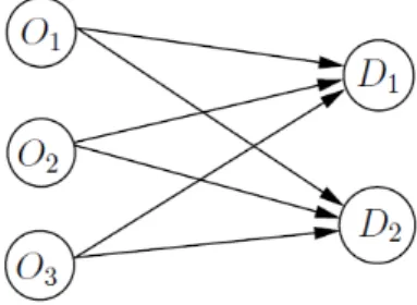
The discrete optimal transportation problem is one that minimizes the cost of transporting a certain amount of goods fromn origins to m destinations. A graphical representation of this problem is shown in figure2.2.
Figure 2.2: Graph of a transportation problem with 3 origin nodes and 3 destination nodes.
First of all, we are going to see the formulation of the linear optimization problem in order to fix notation and make it easier to understand chapter 3. We denote by oi the amount offered in source node iand by dj the amount demanded by destination node j. Let Cij be the cost of transporting a unit from source i to destination j and call X to the matrix n×m in which each of its components xij corresponds to the variable that indicates the amount transported from the source nodeito the destination node j, then the formulation of the optimal transport problem will be
(OTP) min X
n
X
i=1
m
X
j=1
xijCij
s.t.
m
X
j=1
xij ≤oi, i= 1, . . . , n (2.12)
n
X
i=1
xij ≥dj, j= 1, . . . , m (2.13)
xij ≥0, i= 1, . . . , n, j= 1, . . . , m.
For this problem to have a feasible solution, it must necessarily happen that m
X
j=1
dj ≤
n
X
i=1
m
X
j=1
xij ≤
n
X
i=1
2.5. Algorithms 31
that is, total offer must always be greater or equal than total demand.
Among all optimal transportation problems, those that are balanced (those with
Pn
i=1oi =
Pm
j=1dj) are of special importance to us. When we are in this situation,
we can replace the inequalities in the restrictions (2.12) and (2.13) with equalities and the problem (OTP) will be equivalent to
(BTP) min X
n
X
i=1
m
X
j=1
xijCij
s.t.
m
X
j=1
xij =oi, i= 1, . . . , n
n
X
i=1
xij =dj, j= 1, . . . , m
xij ≥0, i= 1, . . . , n, j= 1, . . . , m.
The importance of these problems is that the algorithm we are going to describe in this section can only be applied when the problem we want to solve is balanced. Occasionally
we find problems that are not balanced, i.e., n
X
i=1
oi >
m
X
j=1
dj. In these cases we can
transform the unbalanced problem into an equivalent balanced problem. To do this, an artificial demand node with zero costs is added: ci(m+1)= 0 for i= 1;. . . , nwith demand
dm+1 =
n
X
i=1
oi−
m
X
j=1
dj and the problem can be written in a standard form.
min X
n
X
i=1
m+1
X
j=1
xijCij
s.t.
m+1
X
j=1
xij =oi, i= 1, . . . , n
n
X
i=1
xij =dj, j= 1, . . . , m+ 1
xij ≥0, i= 1, . . . , n, j= 1, . . . , m+ 1.
32 Chapter 2. Preliminaries
If we denote by Πij the amount transported between xi and yj, we take
m
X
j=1
Πij = pi; i= 1, . . . , n,
n
X
i=1
Πij = qj; j= 1, . . . , m
and assume that
Πij ≥0; i= 1, . . . , n; j= 1, . . . , m,
then, writing the expected value in (2.10) as
E((X−Y)p) =
n
X
i=1
m
X
j=1
|xi−yj|pΠij,
we have
Wpp(P, Q) = min
Π
n
X
i=1
m
X
j=1
|xi−yj|pΠij
s.t.
m
X
j=1
Πij =pi; i= 1, . . . , n
n
X
i=1
Πij =qj; j= 1, . . . , m
Πij ≥0; i= 1, . . . , n; j= 1, . . . , m.
that is a problem of the same type as (BTP).
Now we describe the algorithm. We start from a balanced problem (an unbalanced problem can be easily reformulated into this case). We need a feasible initial solution to start working with. This solution is obtained using a heuristic algorithm. There are already several heuristic algorithms described in the literature and we will see below some of them. This solution is known as a feasible initial solution. In order to reach the optimum from the initial solution, we must obtain new solutions in an iterative way that bring us closer and closer to the optimum (that is to say, we will obtain solutions whose total cost is lower and lower) until we reach it. These new solutions will be obtained by the method called MODI (Bazaraa et al. (2010)). This procedure is known as the simplex method for transportation problem.
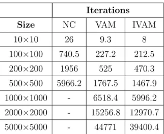
For calculating the initial basic solution there are several heuristics in the literature, the best known are thenorthwest corner denoted as NC andVogel approximation method
2.5. Algorithms 33
as we will see later, is the one that obtains the best resolution times, especially when the problem we want to solve is a big one.
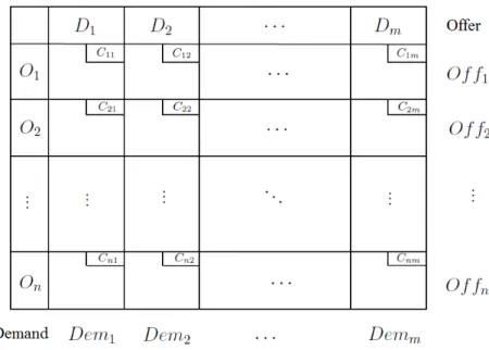
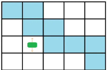
To apply these heuristics we have to start by building what is known as a transportation tableau. To elaborate this table we have to put in the first column the origin nodes and in the first row the target nodes, each square of the table will have in the upper right corner a rectangle with the cost of going from the origin node of the row in which we are to the destination node of the corresponding column. Finally, outside the table we write the offer vector on a column to the right and the demand vector on a row below the table. An example of transportation tableau is shown in Figure2.3.
Figure 2.3: Transportation tableau.
This table will be filled according to the heuristic algorithm that we choose until we obtain the basic initial solution. The number that will appear in each cell will be the quantity of goods that we transport between the source node and the destination node of the row and the column in which the cell is.