The Role of the Risk-Neutral Jump Size Distribution in Single-Factor Interest Rate Models

(1)

Research Article

The Role of the Risk-Neutral Jump Size Distribution in

Single-Factor Interest Rate Models

L. Gómez-Valle and J. Martínez-Rodríguez

Departamento de Econom´ıa Aplicada, Facultad de Ciencias Econ´omicas y Empresariales, Universidad de Valladolid, Avenida del Valle de Esgueva 6, 47011 Valladolid, Spain

Correspondence should be addressed to J. Mart´ınez-Rodr´ıguez; [email protected]

Received 23 December 2014; Accepted 6 May 2015

Academic Editor: Benito M. Chen-Charpentier

Copyright © 2015 L. G´omez-Valle and J. Mart´ınez-Rodr´ıguez. This is an open access article distributed under the Creative Commons Attribution License, which permits unrestricted use, distribution, and reproduction in any medium, provided the original work is properly cited.

We obtain a result that relates the risk-neutral jump size of interest rates with yield curve data. This function is unobservable; therefore, this result opens a way to estimate the jump size directly from data in the markets together with the risk-neutral drift and jump intensity estimations. Then, we investigate the finite sample performance of this approach with a test problem. Moreover, we analyze the effect of estimating the risk-neutral jump size instead of assuming that it is artificially absorbed by the jump intensity, as usual in the interest rate literature. Finally, an application to US Treasury Bill data is also illustrated.

1. Introduction

In the literature, financial variables such as foreign exchange rates, stock prices, and interest rates are usually assumed to follow a diffusion process with continuous paths when pricing financial derivatives. Although they are very attractive because of their statistical properties and computational convenience for theoretical derivation, [1–3] and others found evidence indicating the presence of jumps in stock and interest rate processes. Moreover, jump-diffusion processes are particularly important in pricing and hedging financial derivatives because ignoring jumps in financial prices could cause pricing and hedging risks [2].

In traditional jump-diffusion interest rate models the drift, volatility, jump, and market prices of risk are usually specified as simple parametric functions for pure simplicity and tractability. Most models combine well-known paramet-ric diffusion models with different jump size distributions, for example, [4–6]. Furthermore, the functions of the models are usually chosen to obtain a closed-form solution for the pricing problem. As a result, [1,7,8] proposed nonparametric jump-diffusion models of the short rates that nest most jump-diffusion processes, but a closed-form solution to the pricing problem cannot be obtained. Nevertheless, there are

a lot of efficient numerical methods to provide accurate approximated solutions to the pricing problem.

In order to obtain the yield curves when a closed-form solution is not known, the Monte Carlo method is often used in the literature because of its simplicity and properties. For its implementation, it is necessary to know the value of the interest rate functions and the market prices of risk previously. Hence, estimation is the very first step in the appli-cation and analysis of interest rate models. The estimation of the interest rate functions can be done with interest rate data in the markets; however the market prices of risk are not observable. Therefore, the market prices of risk can only be estimated when a closed-form solution is known for the pricing model. However, in diffusion models there are other alternatives such as the one proposed by [9] which consists of estimating the risk-neutral drift directly from market data.

Recently, in jump-diffusion models [10] proposed a procedure for estimating the risk-neutral drift and jump intensity of interest rates directly from data in the markets, and therefore, the market prices of risk did not have to be estimated for pricing. As usual in the term structure literature, they assumed that the jump size distribution did not change with the risk-neutral measure. That is, the market price of risk was assumed to be artificially absorbed by

(2)

the change in jump intensity from the physical measure to the risk-neutral measure.

The main goal of this paper is to analyze the role of the estimation of the risk-neutral jump size distribution in a term structure model. First, we prove a result that allows us to estimate the risk-neutral jump size directly from market data in a jump-diffusion model. Then, we show the importance of this fact by means of some numerical experiments. Finally, we show the performance of this new approach in a nonparamet-ric jump-diffusion term structure model with US interest rate data.

This approach can be used for parametric as well as nonparametric models. In this paper, we use a nonparametric method such as a kernel method to avoid any arbitrary restriction in the whole model.

The rest of the paper is organized as follows.Section 2 presents the jump-diffusion interest rate model to be studied and shows a new approach for estimating the jump size distri-bution of the risk-neutral interest rates by means of the slope of the yield curve and zero-coupon bonds with numerical dif-ferentiation.Section 3analyzes the finite sample performance of this approach using a nonparametric method.Section 4 examines empirically the behavior of this approach with US interest rate data. Conclusions are contained inSection 5.

2. The Jump-Diffusion Model

In this section, we present a jump-diffusion term structure model with a single state variable. Although one-factor mod-els have several shortcomings, they are still very attractive for practitioners and academics because they offer a unifying tool for the pricing of many interest rate derivatives.

Let (Ω,F,P, {F(𝑡)}_𝑡≥₀) be a filtered probability space satisfying the usual conditions. The price of an interest rate security is driven by the instantaneous interest rate, which follows a mixed jump-diffusion stochastic process of the type:

𝑑𝑟 (𝑡) = 𝜇 (𝑟 (𝑡)) 𝑑𝑡 + 𝜎 (𝑟 (𝑡)) 𝑑𝑊 (𝑡)

+ 𝐽 (𝑟 (𝑡) , 𝑌 (𝑡)) 𝑑𝑁 (𝑡) , (1)

where 𝜇(𝑟) is the drift, 𝜎(𝑟) is the volatility, 𝐽(𝑟, 𝑌) is a function of the instantaneous interest rate and the magnitude of the jump𝑌, which is a random variable with probability distributionΠ,𝑊is the Wiener process, and 𝑁represents a Poisson process with intensity𝜆(𝑟). We assume that𝜇,𝜎,

𝜆 and𝐽 satisfy enough technical regularity conditions: see [11]. Moreover, 𝑑𝑊 is assumed to be independent of 𝑑𝑁, which means that the diffusion component and the jump component of the short-term interest rates are independent of each other. We assume that jump magnitude and jump arrival times are uncorrelated with the diffusion part of the process. The price at time 𝑡, under the above assumptions, of a zero-coupon bond maturing at time 𝑇, with 𝑡 ≤ 𝑇, can be expressed as 𝑃(𝑡, 𝑟; 𝑇). This bond is assumed to have a maturity value of one unit, that is,

𝑃 (𝑇, 𝑟; 𝑇) =1. (2)

We also assume that there exists a new measure Q, equivalent toP, such that the price of a zero-coupon bond is

𝑃 (𝑡, 𝑟; 𝑇) = 𝐸Q[exp(− ∫

𝑇

𝑡 𝑟 (𝑢) 𝑑𝑢) |F(𝑡)] , (3)

where𝐸Q denotes the conditional expectation under theQ measure which is known as risk-neutral probability measure. UnderQ, the short-rate𝑟follows the process:

𝑑𝑟 = (𝜇 (𝑟) − 𝜎 (𝑟) 𝜃𝑊(𝑟) + 𝜆Q(𝑟) 𝐸Q_𝑌[𝐽 (𝑟, 𝑌)]) 𝑑𝑡

+ 𝜎 (𝑟) 𝑑𝑊Q(𝑡) + 𝐽 (𝑟, 𝑌) 𝑑 ̃𝑁Q(𝑡) , (4)

where 𝑊Q is the Wiener process under Q, 𝜃𝑊 is the market price of risk of the Wiener process,𝑁̃Q represents the compensated Poisson process under Q measure with intensity𝜆Q, andΠQ is the jump size distribution underQ. We assume in the change of measure

𝑑𝑊Q= 𝑑𝑊 + 𝜃𝑊𝑑𝑡,

𝜆Q= 𝜃𝑁𝜆,

ΠQ_{= 𝜃}𝑌_Π,

(5)

where 𝜃𝑁 and 𝜃𝑌 are the market prices of risk of jump intensity and jump size, respectively; see [12].

In the absence of a jump component, the term structure equation can be obtained by means of a riskless portfolio of two bonds with different maturities and imposing the absence of arbitrage condition. However, in the presence of a jump component, the no-arbitrage argument can no longer be applied, as jump risk cannot be diversified away using traded bonds [13]. Therefore, the valuation of fixed income securities in a jump-diffusion model requires a transition from the actual to the equivalent martingale measure. In general, this task can be accomplished by specifying a stochastic discount factor for the economy and can be used directly to obtain the term structure equation consistent with the process given in (1). Thus, the pricing partial integrodifferential equation is as follows:

𝑃_𝑡(𝑡, 𝑟) + (𝜇 (𝑟) − 𝜃𝑊(𝑟) 𝜎 (𝑟)) 𝑃𝑟(𝑡, 𝑟)

+1

2𝜎

2_{(𝑟) 𝑃}

𝑟𝑟(𝑡, 𝑟) − 𝑟𝑃 (𝑡, 𝑟)

+ 𝜆Q(𝑟) 𝐸Q_𝑌[𝑃 (𝑡, 𝑟 + 𝐽) − 𝑃 (𝑡, 𝑟)] =0;

(6)

see [13] for more details about obtaining this partial differen-tial equation. This pricing equation is the same for all interest rate derivatives; we only have to add the corresponding final conditions.

In order to obtain the term structure,𝜇,𝜎,𝜃𝑊,𝜆Qand the parameters of the distributionΠQ must be estimated. Then, these functions are replaced in the pricing equation(6)which is solved by taking into account the final condition(2).

Finally, the yield curve can be expressed as

(3)

In the literature, to the best of our knowledge, there is no approach to estimating the market prices of risk𝜃𝑊,𝜃𝑁, and𝜃𝑌 for a jump-diffusion model, except if a closed-form solution is known. References [1, 7] show how to estimate

𝜇,𝜎, and𝜆by means of moment equations with data in the markets. However, this approach does not allow us to estimate the market prices of risk, which are necessary to price interest rate derivatives, but they are not observable. Recently, [10] proposed a new approach for estimating the risk-neutral drift and jump intensity directly from market data and, hence, the market prices of risk do not have to be estimated. They proved the following result.

Theorem 1. Let𝑃(𝑡, 𝑟; 𝑇)be a solution to(6)subject to(2), and

𝑟follows a jump-diffusion stochastic process given by(4); then,

𝜕𝑅

𝜕𝑇󵄨󵄨󵄨󵄨󵄨󵄨󵄨󵄨𝑇=𝑡

= 1

2(𝜇 (𝑟) − 𝜎 (𝑟) 𝜃

𝑊_{(𝑟) + 𝜆}Q_{(𝑟) 𝐸}Q

𝑌[𝐽 (𝑟, 𝑌)]) ,

(8)

𝜕 (𝑟2_𝑃)

𝜕𝑇 󵄨󵄨󵄨󵄨 󵄨󵄨󵄨󵄨

󵄨󵄨󵄨𝑇=𝑡

= − 𝑟3(𝑡) +4𝑟 (𝑡) 𝜕𝑅

𝜕𝑇󵄨󵄨󵄨󵄨󵄨󵄨󵄨󵄨𝑇=𝑡+ 𝜎

2_(𝑟)

+ 𝜆Q(𝑟) 𝐸Q_𝑌[𝐽2(𝑟, 𝑌)] .

(9)

Reference [10] assumed that the jump size distribution underQwas known and equal to the distribution underP; that is,𝜃𝑌 =1. In this paper, we take one step ahead and we propose the following result to estimate the risk-neutral jump size distribution directly from yield curve data.

Theorem 2. Let 𝑃(𝑡, 𝑟; 𝑇)be a solution to(6)subject to (2), and𝑟follows a jump-diffusion stochastic process given by(4); then,

𝜕 (𝑟3𝑃)

𝜕𝑇 󵄨󵄨󵄨󵄨 󵄨󵄨󵄨󵄨

󵄨󵄨󵄨𝑇=𝑡

= − 𝑟4(𝑡) +6𝑟2(𝑡) 𝜕𝑅

𝜕𝑇󵄨󵄨󵄨󵄨󵄨󵄨󵄨󵄨𝑇=𝑡+3𝑟 (𝑡) 𝜎

2_(𝑟)

+3𝑟 (𝑡) 𝜆Q(𝑟) 𝐸Q_𝑌[𝐽2(𝑟, 𝑌)]

+ 𝜆Q(𝑟) 𝐸Q_𝑌[𝐽3(𝑟, 𝑌)] .

(10)

Theorems 1and 2allow us to estimate the risk-neutral drift, jump intensity, and jump size distribution of the interest rates by means of the prices of zero-coupon bonds and the slope of the yield curves and, hence, we do not have to estimate the market prices of risk.

Finally, notice that any parametric or nonparametric technique can be applied to estimate the slopes. In this paper, in order to illustrate these results we will use the Nadaraya-Watson nonparametric estimator. Suppose a dataset consists of𝑁pairs of observations(𝑟₁, 𝑋₁), . . . , (𝑟_𝑁, 𝑋_𝑛), where𝑟_𝑖 is the explanatory variable and𝑋_𝑖is the response variable. We assume a model of the kind𝑋_𝑖 = 𝑔(𝑟_𝑖) + 𝜖_𝑖, where𝑔(𝑟)is

an unknown function and𝜖_𝑖 is an error term, representing random errors in the observations or variability from sources not included in𝑟_𝑖. The errors𝜖_𝑖 are assumed to be independent and identically distributed with mean 0 and finite variance. The estimate is given by

̂𝑔(𝑟) =∑𝑁𝑖=1𝑤𝑖(𝑟) 𝑋𝑖

∑𝑁_𝑖=₁𝑤_𝑖(𝑟) , (11)

with positive weights𝑤_𝑖(𝑟) = 𝐾((𝑟 − 𝑟_𝑖)/ℎ)(e.g., the Gaussian kernel which is widely used in the literature and we use it in this paper) andℎis the bandwidth; see [14].

3. Numerical Experiments

In this section, we consider a test problem in order to inves-tigate the effect of the estimation of the risk-neutral jump size in a yield curve pricing problem.

As a basic test problem, we consider a jump extended square root process with exponential jumps which is denoted as CIR-EJ:

𝑑𝑟 = 𝛽 (𝑚 − 𝑟) 𝑑𝑡 + 𝜎√𝑟𝑑𝑊 (𝑡) + 𝑌 (𝜂) 𝑑𝑁 (𝑡) , (12)

where the jump size,𝑌, is distributed exponentially with a positive mean𝜂,𝑌 󴁄󴀼 Exp(𝜂). The market prices of risk of this pricing model are as follows:

𝜃𝑊_{(𝑟) =} 𝜃

𝜎√𝑟, (13)

𝜃𝑁= 𝜑, (14)

𝜃𝑌= 𝜙. (15)

This model is a slight modification of the one proposed by [13] and used by [15] for pricing American interest rate options. The closed-form solution of this problem is very similar to the one obtained by [13] just replacing𝜂by𝜂Q. The only reason we choose this model for our numerical experiments is because a closed-form solution is known and, therefore, we can obtain the exact yield curves to make some comparisons.

In our implementation, we assume that the market prices of risk parameters take values coherent with those in the literature:𝜃 = −0.167,𝜑 = 0.5, and 𝜙 = 0.9. Next, we combine them with the values of the parameters used by [15] to price zero-coupon bonds and American interest rate options. Therefore, we assume that 𝛽 = 0.267,𝑚 = 0.03,

𝜎 =0.075,𝜆 =2, and𝜂 =0.01.

(4)

In order to analyze the effect of estimating each risk-neutral interest rate function within the CIR-EJ model, we will consider different assumptions.

(i) Assumption A1. We assume that the drift, the jump intensity, and the jump size distribution of the compensated interest rate process under Q, the risk-neutral measure, are equal to the drift, the jump intensity, and jump size distribution underPmeasure. This means that the market prices of risk parameters in the CIR-EJ model are as follows:

𝜃 =0 and𝜑 = 𝜙 =1. Consider

𝜂Q= 𝜂,

𝜆Q_{(𝑟) = 𝜆 (𝑟) ,}

𝜇Q(𝑟) = 𝜇 (𝑟) + 𝜂𝜆 (𝑟) ,

(16)

where𝜇Q(𝑟) = 𝜇(𝑟)−𝜎(𝑟)𝜃𝑊(𝑟)+𝜆Q(𝑟)𝐸_𝑌Q(𝐽(𝑟, 𝑌))is the risk-neutral drift of the compensated interest rate process.

(ii) Assumption A2.We assume that the risk-neutral jump intensity and size are equal to the jump intensity and size underPmeasure. However, we assume that the risk-neutral drift is different underPmeasure. That is, the market price of risk associated with the Brownian motion is(13), but𝜑 =

𝜙 =1. One has

𝜂Q = 𝜂,

𝜆Q(𝑟) = 𝜆 (𝑟) ,

𝜇Q(𝑟) = 𝜇 (𝑟) − 𝜃𝑟 + 𝜂𝜆 (𝑟) .

(17)

(iii) Assumption A3.We assume that the risk-neutral jump intensity is equal to the jump intensity under thePmeasure. However, the risk-neutral drift and jump size are different from the drift and jump size under thePmeasure. That is, the market prices of risk associated with the Brownian motion and jump size are (13) and (15), respectively, but 𝜑 = 1. Consider

𝜂Q= 𝜙𝜂,

𝜆Q(𝑟) = 𝜆 (𝑟) ,

𝜇Q_{(𝑟) = 𝜇 (𝑟) − 𝜃𝑟 + 𝜙𝜂𝜆 (𝑟) .}

(18)

(iv) Assumption A4.We assume that the risk-neutral jump size is equal to the jump size underPmeasure. However, the risk-neutral drift and jump intensity are different from the drift and jump intensity under thePmeasure. That is, the market prices of risk associated with the Brownian motion and jump intensity are(13)and(14), respectively, but𝜙 =1. Consider

𝜂Q= 𝜂,

𝜆Q(𝑟) = 𝜑𝜆 (𝑟) ,

𝜇Q(𝑟) = 𝜇 (𝑟) − 𝜃𝑟 + 𝜂𝜑𝜆 (𝑟) .

(19)

See [10] for more details.

(v) Assumption A5. The risk-neutral drift, jump intensity, and jump size of the compensated interest rate process are different from the drift, the jump intensity, and the jump size underPmeasure. That is, the market prices of risk associated with the Brownian motion, jump intensity, and jump size are (13),(14), and(15), respectively. One has

𝜂Q= 𝜙𝜂,

𝜆Q(𝑟) = 𝜑𝜆 (𝑟) ,

𝜇Q(𝑟) = 𝜇 (𝑟) − 𝜃𝑟 + 𝜙𝜂𝜑𝜆 (𝑟) .

(20)

In order to make comparisons of the different assump-tions, we obtain the exact yield curves with the CIR-EJ model and the approximated yield curves with the different assumptions and the data. However, previously, we have to estimate all the functions in the models.

Under Assumption A1, we have to estimate all the interest rate functions under the P measure. Therefore, we can use interest rate observations and the moment equations technique by [1,7]

𝑀1(𝑟) = lim

Δ𝑡 →0𝐸 [𝑟 (𝑡 + Δ𝑡) − 𝑟 (𝑡) |F(𝑡)]

= 𝜇 (𝑟) + 𝜆 (𝑟) 𝐸𝑌[𝐽] ,

𝑀2(𝑟) = lim

Δ𝑡 →0𝐸 [(𝑟 (𝑡 + Δ𝑡) − 𝑟 (𝑡))

2_|_F_(𝑡)]

= 𝜎2(𝑟) + 𝜆 (𝑟) 𝐸_𝑌[𝐽2] ,

𝑀𝑘(𝑟) = lim

Δ𝑡 →0𝐸 [(𝑟 (𝑡 + Δ𝑡) − 𝑟 (𝑡))

𝑘 _|_F_(𝑡)]

= 𝜆 (𝑟) 𝐸𝑌[𝐽𝑘] , 𝑘 ≥3;

(21)

see [7] for regularity conditions and limiting distributions. In our test problem, we have assumed that the jump size

𝑌is distributed exponentially; thus,

𝐸_𝑌[𝑌𝑘] = 𝜂𝑘𝑘!, 𝑘 =1,2,3, . . . . (22)

We replace(22)in(21)and obtain the moment conditions necessary to estimate the interest rate coefficients for the CIR-EJ process. See [1,7] for a similar approach, but with other jump size distributions.

(5)

Table 1: RMSE with the different approaches for the 5000 simulated yield curves with𝑁 =7500 andΔ𝑡 =1/250.

Assumption 6 months 9 months 12 months 18 months 24 months

A1 9.4249 × 10−3 1.3762 × 10−2 1.7264 × 10−2 2.3932 × 10−2 2.9652 × 10−2

A2 1.9306 × 10−3 2.7565 × 10−3 3.5392 × 10−3 4.6897 × 10−3 5.5389 × 10−3

A3 1.0672 × 10−3 1.5158 × 10−3 1.9098 × 10−3 2.4730 × 10−3 2.8823 × 10−3

A4 8.3666 × 10−4 1.1984 × 10−3 1.5177 × 10−3 1.9240 × 10−3 2.2226 × 10−3

A5 7.6592 × 10−4 1.1215 × 10−3 1.4277 × 10−3 1.8391 × 10−3 2.1277 × 10−3

the Nadaraya-Watson estimator with a Gaussian kernel. Then, we estimate the rest of functions by means of the moment equations(21)as in A1.

Next, we consider Assumption A3. In this case, we have to estimate the drift and the jump size of the risk-neutral interest rate stochastic process. This process is not observable, but we can use(8) and (9)with numerical differentiation and the Nadaraya-Watson estimator with a Gaussian kernel. First, we estimate the risk-neutral drift as in A2 and, then, we estimate the volatility and the jump intensity with the moment equations as in A1. Finally, we replace these functions in(9) and use yields with maturities of 6 months and 1 year in order to estimate the expected jump size with a second order forward approximation for the derivatives and the Nadaraya-Watson estimator with a Gaussian kernel.

Then, we take into account Assumption A4. We have to estimate the drift and the jump intensity of the risk-neutral compensated interest rate stochastic process. As this process is not observable, we use(8)and(9)with numerical differentiation and the Nadaraya-Watson estimator with a Gaussian kernel in a similar way to that with Assumption A3; see [10] for more details.

Finally, we consider Assumption A5. We have to estimate the drift, the jump size, and the jump intensity of the risk-neutral compensated interest rate stochastic process. Then, we estimate the volatility of the instantaneous interest rates with the moment equations and use(8)–(10)with numerical differentiation and the Nadaraya-Watson estimator with a Gaussian kernel. To be exact, we use yields with maturities of 6 months and 1 year in order to approximate the slope of the yield curve and the products of the interest rates and prices. However, we still have to estimate the volatility of the instantaneous interest rate, but we do it with the moment equations as in A1. In all the cases we use a second order forward approximation to approximate the derivatives.

In order to price zero-coupon bonds we have to solve the pricing equation (6) subject to (2). However, when nonparametric methods are used, it is not possible to find a closed-form solution and a numerical method must be applied to obtain an approximated solution. Therefore, we apply the Monte Carlo method with 10000 simulations and a discretization interval equal to one day. The number of simulations and the discretization interval are chosen to render the Monte Carlo error negligible: see [1].

Throughout this paper, in order to analyze the behavior of the different assumptions, we use the root mean square error:

RMSE= √ 1

𝑁

∑

𝑡=1(𝑅 (𝑡) − ̂𝑅 (𝑡))

2

, (23)

where𝑁is the number of observations,𝑅(𝑡)is the observed or theoretical value, and ̂𝑅(𝑡)is the estimated value with the corresponding model.

Table 1 shows the performance of the different Assumptions A1–A5 that we have taken into account to obtain the yield curves for different maturity times. As it is well known in the literature, the single-factor models do not work very well for long maturities. Hence, we consider maturities until 24 months. When we assume that all the functions of the risk-neutral interest rate are equal to the functions under thePmeasure, Assumption A1, we obtain the highest errors. Under Assumptions A3 and A4, we assume that only two interest rate functions are estimated under the risk-neutral measure: the risk-neutral drift and jump size or the risk-neutral drift and jump intensity. Note that assuming that the risk-neutral drift and jump intensity are different from those under Pmeasure provides lower errors than assuming that the risk-neutral drift and jump size are different underPandQmeasures.

Assumption A4 has usually been considered in the term structure literature; see, for example, [17]. In particular, Assumption A5, where all the functions are estimated assum-ing different values under the risk-neutral measure, provides the lowest errors. Then, the more the functions we estimate under the risk-neutral measure, the lower the errors. We have also repeated these experiments with other parameters and the same conclusions are reached.

Thus, estimating all the risk-neutral functions directly from data in the markets provides more accurate yield curves than assuming some arbitrary market prices of risk for the model.

4. Empirical Analysis

In this section, we analyze the effect of the estimation of the risk-neutral jump size directly from data in the markets in contrast to the assumption that the market price of risk of jump size is artificially absorbed by the change in jump intensity from physical measure to risk-neutral measure by means of US yield curves data.

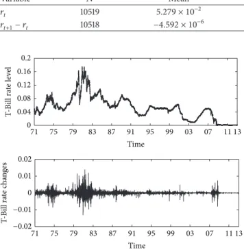
The short rate is inherently unobservable, and it has to be approximated using interest rates of short-term zero-coupon bonds: see [18] for a detailed discussion. In this paper, we use the 3-month Treasury Bill rates because [8] showed that any instrument with maturity below three months should not be used when estimating jump-diffusion processes.

(6)

Table 2: Summary of the statistics of the US 3-month Treasury Bill rates and the first differences, January 1971 to February 2013.

Variable 𝑁 Mean Std. dev. Max. Min.

𝑟𝑡 10519 5.279 × 10−2 3.323 × 10−2 1.752 × 10−1 1.0 × 10−4

𝑟_𝑡+1− 𝑟_𝑡 10518 −4.592 × 10−6 1.067 × 10−3 1.393 × 10−2 −1.321 × 10−2

0.2 0.16 0.12 0.08 0.04 0

71 75 79 83 87 91 95 99 03 07 11 13

Time

71 75 79 83 87 91 95 99 03 07 11 13

Time 0.02

0.01 0 −0.01 −0.02

T-Bi

ll ra

te

c

ha

ng

es

T-Bill ra

te

le

ve

l

Figure 1: The time series of the level and changes in the 3-month Treasury Bill rates, from January 1971 to February 2013.

In order to estimate the risk-neutral drift, jump intensity, and jump size of the interest rates using(8)–(10)and a second order forward difference formula, we need additional data. Then, we use daily observations of the secondary market yields with the shortest maturities available in the Federal Reserve h.15 database. We consider the 6-month Treasury Bills and the yields of 1-year Treasury notes, because we do not have enough observations of the 1-year Treasury Bills for the whole estimation period of time.

All the estimations are done as in Section 3 using the Nadaraya-Watson estimator with a Gaussian kernel. (We use

ℎ𝑟 = ℎ𝜎𝑟 as bandwidth, with the smoothing parameter

ℎ = 1.2 for the second moment and ℎ = 1.5 for higher order moments. In Assumption A4 we useℎ = 1.7 for the nonparametric estimation of the risk-neutral drift and jump intensity, as in [10]. Finally we useℎ = 1.7,ℎ = 0.85, and

ℎ =1.3 for the nonparametric estimation of the risk-neutral drift, jump intensity, and jump size, resp.)

In order to obtain the yield curves we have to solve the pricing equation(6)subject to(2). We use the Monte Carlo method with 5000 simulations and a discretization interval equal to one day, as in [10] in order to be able to make comparisons.

Table 3 shows the RMSE obtained with the different assumptions for the yield curves with the shortest maturities available in the Federal Reserve h.15 database: 6 months, 12 months, and 24 months. First, Assumption A1 provides the highest error inTable 3. This fact means that it is important to estimate the market prices of risk by means ofTheorem 1 and evenTheorem 2in order to obtain accurate yield curves.

Table 3: The RMSE of the yield curves for different maturity times under Assumptions A1–A5.

Assumption 6 months 12 months 24 months

A1 2.9055 × 10−3 5.5931 × 10−3 9.2256 × 10−3

A2 2.6774 × 10−3 4.6240 × 10−3 7.0574 × 10−3

A3 2.6773 × 10−3 4.6239 × 10−3 7.0571 × 10−3

A4 2.6764 × 10−3 4.6224 × 10−3 7.0531 × 10−3

A5 2.6998 × 10−3 4.6487 × 10−3 7.1063 × 10−3

Finally, the errors of Assumptions A2–A5 are very similar; in fact, the differences are just of order 10−5. These differences could be considered as negligible because they can be due to the propagation of errors of the approximations. However, note that small errors in pricing zero-coupon bonds usually provide higher errors when pricing interest rate contingent claims such as bond options. Moreover, we think that it is very difficult to reduce the order of these errors because we are considering a single-factor model. This kind of models is very attractive for practitioners in the markets, but they also have some limitations in order to explain the yield curves in the markets.

5. Conclusions

(7)

the same, although the differences are nearly negligible in the empirical experiments.

Finally, we model separate risk premiums for the diffu-sion, jump size, and jump intensity in a single-factor term structure model. In the numerical experiments we obtain lower errors than when we assume that one of the jump risk premiums is artificially absorbed by the other one. As far as the empirical data is concerned, we find very small differences which could be considered as negligible because they could be due to the propagation of errors as we use three related approximations and a single-factor model. As a future research, we would like to apply this approach to price other interest rate derivatives such as bond options. We think that the differences will be more important and the accurate estimation of the market prices of risk will provide a high improvement in their pricing.

Appendix

This appendix outlines the proof ofTheorem 2.

Proof ofTheorem 2. Let𝐷(𝑡) = 𝑒− ∫0𝑡𝑟(𝑠)𝑑𝑠_{denote the discount} process and then

𝑑𝐷 = − 𝑟𝐷 𝑑𝑡. (A.1)

By means of Ito’s product rule (see [19] and(4)and(A.1)) we obtain

𝑑 (𝑟3𝐷) = 𝐷 (3𝑟2(𝜇 − 𝜎𝜃𝑊+ 𝜆Q𝐸Q_𝑌[𝐽]) − 𝑟4

+3𝑟𝜎2+3𝑟𝜆Q𝐸_𝑌Q[𝐽2] + 𝜆Q𝐸Q_𝑌[𝐽3] ) 𝑑𝑡

+ 𝐷2𝑟𝜎𝑑𝑊Q+ 𝐷 (2𝑟𝐽 + (2𝑟 +1) 𝐽2+ 𝐽3) 𝑑 ̃𝑁Q.

(A.2)

If we take expectation with respect to Qmeasure over the integral form of(A.2), we obtain

𝑟3(𝑇 + ℎ) 𝑃 (𝑡, 𝑟; 𝑇 + ℎ) − 𝑟3(𝑇) 𝑃 (𝑡, 𝑟; 𝑇)

= ∫𝑇+ℎ

𝑇 (3𝑟

2_{(𝜇 − 𝜎𝜃}𝑊_{+ 𝜆}Q_𝐸Q

𝑌[𝐽]) − 𝑟4+3𝑟𝜎2

+3𝑟𝜆Q𝐸Q_𝑌[𝐽2] + 𝜆Q𝐸_𝑌Q[𝐽3]) (𝑠) 𝑃 (𝑡, 𝑟; 𝑠) 𝑑𝑠,

(A.3)

as𝑑𝑊Q and 𝑑 ̃𝑁Q are martingales underQ and taking out what is known as

𝐸Q[𝑟3(𝑠) 𝐷 (𝑠) |F_𝑡]

= 𝑟3(𝑠) 𝐸Q[𝐷 (𝑠) |F_𝑡] = 𝑟3(𝑠) 𝑃 (𝑡, 𝑟; 𝑠) 𝐷 (𝑡) . (A.4)

Dividing byℎand taking limits in(A.3)we can write

𝜕 (𝑟3𝑃)

𝜕𝑇 (𝑡, 𝑟; 𝑇) = (3𝑟2(𝜇 − 𝜎𝜃𝑊+ 𝜆Q𝐸Q𝑌[𝐽]) − 𝑟4

+3𝑟𝜎2+3𝑟𝜆Q𝐸_𝑌Q[𝐽2] + 𝜆Q𝐸Q_𝑌[𝐽3]) (𝑇) 𝑃 (𝑡, 𝑟; 𝑇) .

(A.5)

Finally, setting𝑇 = 𝑡we get(10).

Conflict of Interests

The authors declare that there is no conflict of interests regarding the publication of this paper.

Acknowledgments

This work was supported in part by the GIR Optimización Dinámica, Finanzas Matemáticas y Utilidad Recursiva of the Universidad de Valladolid, and the projects MTM2014-56022-C2-2-P of the Ministerio de Economa y Competitivi-dad de España and VA191U13 of the Junta de Castilla y León. The authors gratefully acknowledge the helpful comments of an anonymous referee.

References

[1] M. Johannes, “The statistical and economic role of jumps in continuous-time interest rate models,”The Journal of Finance, vol. 59, no. 1, pp. 227–260, 2004.

[2] B.-H. Lin and S.-K. Yeh, “Jump-diffusion interest rate process: an empirical examination,” Journal of Business Finance & Accounting, vol. 26, no. 7-8, pp. 967–995, 1999.

[3] K. Park, C. M. Ahn, and R. Fujihara, “Optimal hedged portfo-lios: the case of jump-diffusion risks,”Journal of International Money and Finance, vol. 12, no. 5, pp. 493–510, 1993.

[4] C. Ahn and H. Thompson, “Jump-processes and the term structure of interest rates,”The Journal of Finance, vol. 43, pp. 155–174, 1998.

[5] J. Baz and S. R. Das, “Analytical approximations of the term structure for jump-diffusion processes: a numerical analysis,” The Journal of Fixed Income, vol. 6, no. 1, pp. 78–86, 1996. [6] N. A. Beliaeva, S. K. Nawalkha, and G. M. Soto, “Pricing

Amer-ican interest rate options under the jump-extended Vasicek model,”The Journal of Derivatives, vol. 16, no. 1, pp. 29–43, 2008. [7] F. M. Bandi and T. H. Nguyen, “On the functional estimation of jump-diffusion models,”Journal of Econometrics, vol. 116, no. 1-2, pp. 293–328, 2003.

[8] C. Mancini and R. Reno, “Threshold estimation of Markov models with jumps and interest rate modeling,” Journal of Econometrics, vol. 160, no. 1, pp. 77–92, 2011.

[9] L. G´omez-Valle and J. Mart´ınez-Rodr´ıguez, “Modelling the term structure of interest rates: an efficient nonparametric approach,”Journal of Banking and Finance, vol. 32, no. 4, pp. 614–623, 2008.

[10] L. G´omez-Valle and J. Mart´ınez-Rodr´ıguez, “Estimation of risk-neutral processes in single-factor jump-diffusion interest rate models,”Journal of Computational and Applied Mathematics, 2015.

[11] B. Øksendal and A. Sulem,Applied Stochastic Control of Jump Diffusions, Springer, Berlin, Germany, 2005.

[12] W. J. Runggaldier, “Jump-diffusion models,” inHandbook of Hevay Tayled Distributions in Finance, S. T. Rachev, Ed., pp. 169–209, Universitat Karisruhe, North Holland, Karisruhe, Germany, 2003.

[13] S. K. Nawalkha, N. Beliaeva, and G. Soto, Dynamic Term Structure Modeling, John Wiley & Sons, 2007.

(8)

[15] N. Beliaeva and S. K. Nawalkha, “Pricing American interest rate options under the jump-extended constant-elasticity-of-variance short rate models,”Journal of Banking and Finance, vol. 36, no. 1, pp. 151–163, 2012.

[16] E. Platen and N. Bruti-Liberati,Numerical Solution of Stochas-tic Differential Equations with Jumps in Finance, vol. 64 of Stochastic Modelling and Applied Probability, Springer, Berlin, Germany, 2010.

[17] S. R. Das and S. Foresi, “Exact solutions for bond and option prices with systematic jump risk,”Review of Derivatives Research, vol. 1, no. 1, pp. 7–24, 1996.

[18] D. A. Chapman, J. B. Long Jr., and N. D. Pearson, “Using proxies for the short rate: when are three months like an instant?” Review of Financial Studies, vol. 12, no. 4, pp. 763–806, 1999. [19] S. E. Shreve,Stochastic Calculus for Finance II: Continuous Time

(9)

Submit your manuscripts at

http://www.hindawi.com

Hindawi Publishing Corporation

http://www.hindawi.com Volume 2014

Mathematics

Journal of

Mathematical Problems in Engineering

Hindawi Publishing Corporation http://www.hindawi.com

Differential Equations International Journal of

Volume 2014

http://www.hindawi.com Volume 2014 Hindawi Publishing Corporationhttp://www.hindawi.com Volume 2014

Mathematical PhysicsAdvances in

Complex Analysis

Journal of

Optimization

Journal of Hindawi Publishing Corporation

Combinatorics

International Journal of

Journal of

Function Spaces

Abstract and Applied Analysis Hindawi Publishing Corporation

International Journal of Mathematics and Mathematical Sciences

Hindawi Publishing Corporation http://www.hindawi.com Volume 2014

The Scientific

World Journal

Discrete Dynamics in Nature and Society

Discrete Mathematics

Journal of

http://www.hindawi.com Volume 2014 Hindawi Publishing Corporationhttp://www.hindawi.com Volume 2014

The Role of the Risk-Neutral Jump Size Distribution in Single-Factor Interest Rate Models

Research Article