STUDIES FOR TYPE-I, TYPE-II AND TYPE-III INTERMITTENCIES
Sergio Elaskara, Ezequiel del Riob and José M. Donosob
"Departamento de Aeronáutica, Universidad Nacional de Córdoba and CONICET, Av. Vélez Sarfield 1611, Córdoba, Argentina, [email protected]
b Escuela Técnica Superior de Ingenieros Aeronáuticos, Universidad Politécnica de Madrid, Plaza Cardenal Cisneros 3, Madrid, España, [email protected]
Keywords: intermittency, chaos, reinjection
1 INTRODUCTION
Intermittency is a particular form of deterministic chaos, in which transition between laminar and chaotic phases occurs. A system is in regular behavior until, with a small change in a parameter, it begins to show chaotic burst at irregular intervals. Pomeau and Maneville introduced the intermittency concept in relation to the Lorenz system (Maneville and Pomeau, 1979; Pomeau and Maneville, 1980; Maneville, 1980). In this work we pay attention to this phenomenon since it is well-known that it emerges in several topics in the frame of the fluid mechanics, such as Lorenz system, Rayleigh-Bénard convection; derivative non-lineal Schoendinger equation and turbulence, among others.
The so-called intermittency phenomenon is classified into three types: I, II and III, according to the Floquet multipliers or eigenvalue in the local Poincaré map. For continuous-time system, the type-I intermittency arises in a cyclic-fold bifurcation, for which a stable and an unstable orbits collapse, therefore, the system loses the stable orbits in the vicinity of the vanished periodic orbits. For some maps, type-I intermittency occurs by means of an inverse tangent bifurcation, in this case an eigenvalue leaves the unit circle through +1. Intermittency type-II begins in a subcritical Hopf bifurcation, so that, two complex-conjugate Floquet multipliers or two complex-conjugate eigenvalues of the local Poincaré map exit in the unit circle. Intermittency of type-Ill is related to a subcritical period-doubling or flip bifurcation and one Floquet multiplier leaves the unit circle through -1.
In some previous papers, we have presented a new methodology to evaluate the main defining properties for type-II and type-Ill intermittencies, such as the reinjection probability density function (RPD), the probability density of the laminar phase, the average laminar length and the characteristic relation (del Rio and Elaskar, 2009 and 2010; del Rio, et ah, 2010; Elaskar and del Rio, 2009; Elaskar et ah, 2010). In this work we extend this procedure to the type-I intermittency.
The local Poincaré maps for type-I, II and III intermittencies are usually written as
xn+l=(l + e)xn+axl with a>0 (1)
xn+l=-(l + e)xn-ax3n
for which the intermittency phenomenon exists only for s > 0 (Rusbend, 1990; Shuster and Just, 2005; Kim etah, 1997 and 1997a).
which gives §(x) = 8 (x -A). We refer here another interesting case where it was considered (j)(x) oc 1 / Vx - A to study type-III intermittency in a electronic circuit (Won, et al. 2003).
Due to the disparity observed in modeling §, we can conclude that it is very important to provide a method to obtain a correct form for the RPD for each different map, because once the RPD function is properly stated, it can be possible to describe some other characteristic parameters for the intermittency phenomenon. In the next section we present the new method to derive the RPD function for types I, II and III intermittencies by using numerical data. This technique can be also extrapolated to use the experimental data for the same purpose.
2 NEW METHODOLOGY TO EVALUATE THE REINJECTION PROBABILITY DISTRIBUTION
In this paper, we do not directly measure the reinjection probability density §(x) from the numerical data, instead of this, we numerically compute the function M(x), defined as
I T (|)(T) dx
M(x) = ^ / / <|)(T)*0; M ( X ) = 0 / / <|)(T) = 0 (2)
where x¡ is the closed point to the unstable fixed point where the reinjection takes place, i.e. it is the lower bound of the reinjection. The integration interval [x¡, c] defines the laminar region. M{x) has been calculated for a broad class of maps numerically, and it has been stated that if exhibits the linear form
M(x) = mx + Xh (3)
as a very good approximation. This form generalizes the function introduced by del Rio and Elaskar (2009). From Eq.(2) it possible to determine that M(x¡) = x¡, then, it verifies
M(x) = w ( x - x . ) + x. (4)
where the slope m plays an important role in the intermittency dynamics. Therefore, the function M(x) has been proved to be an useful tool to study type-II and type-III intermittencies. From Eq.(4) and Eq.(2) the reinjection probability density can be deduced, giving
§(x) = A ( x - xi)a with a = , (5)
m-\
where A is the normalization constant, which can be written as
( c - x;) l - «v
m must satisfy the condition 0 < m < 1 which has been met in all our numerical tests. The usual uniform probability reinjection is recovered for m = 0.5 with x¡ = 0, leading to M{x) = 0.5 x.
3 APPLICATION TO INTEMITTENCY TYPE-I
The new technique is now applied to study the type-I intermittency using the illustrating map
* „+i = £ + x „ + a x „ ' / x„ < X,
«+1
* *1
v ! ~ xi J
if
(7)
x„ < x,
where x¡ is such that s + x¡+axf = 1. For s = 0 the origin is a fixed point, however, for s >0
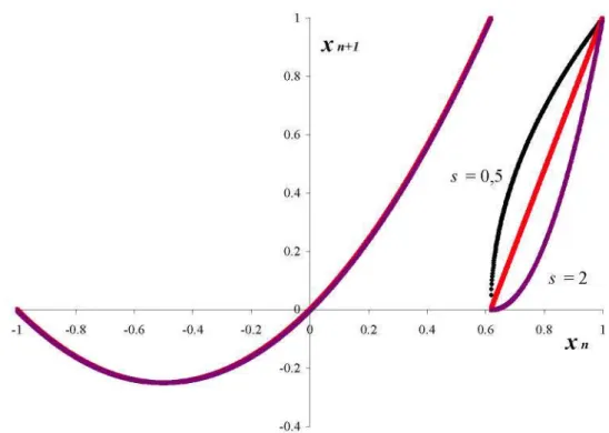
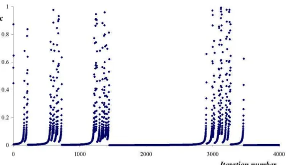
all points x close to the origin move away in a process driven by the parameters s and a. When the n-th iterated value x„ approaches x¡ the reinjection mechanism starts, governed by exponent s. Figure 1 shows the map (7) for s = 0.5, 1 and 2 for the black, red and purple lines respectively, and Figure 2 shows the map time evolution of the laminar and chaotic behaviors with irregular lasting. Figure 3 depicts the bifurcation diagram to illustrate the instability at s=0, for a = 1, s = 2.
-0.4 J
1 X
0.8
0.6
0.4
-0.2 -
i--it» i
. • • • . . • <
* . \
ti Jl J*
1000 2000
» •
• •
3000 4000
Iteration number
Figure 2. Eq.(7) map time evolution for e = 0.000001, a = 1, s = 2.
X 1 1
0.5
-0 6
0.4
0.2
-0
0?.
*
1 t
t f
1
t 1
1 1 1 1 1 1
-0.02 -0.015 -0.01 -0.005 0.005 0.01
Figure 3. Bifurcation diagram for Eq.(3). s = 2 and a=\.
3.1 Reinjection probability density function
0.12
M(x)
o.i
0.08
-s = 0,75 ..•••
0.06
-0.04 0.02
....••:::::-•••
rrT
. . . , : : : : -: :
-,^€:'
~ I I I I I I I I I I
0 0.02 0.04 0.06 0.08 0.1 0.12 0.14 0.16 0.18 0.2
Figure 4. Function M(x). s = 0.75; 1 and 2; a = 1 and e = 0.000001.
After applying the least square method, we have obtained the corresponding m values of theM slope and each exponent a appearing in Eq.(5), as follows
5 = 0.75, m = 0.5686 a = 0.318
5=1.0, w = 0.4936^0.5 a =-0.02516^0 5 = 2.0, m = 0.3104 a =-0.55
In this kind of intermittency, k=l, the RPD normalization reads
f ° §{x) dx = f ° A xadx = 1, (8)
which convergences for a > -1, giving for A the expression
a + 1 A: ^a+1
m
\-m
^mi(m-Y)
(9)
and the RPD for type-I intermittency is finally given by
<KX): m cml(m-\) x m_x _ a + 1 ^Q,
1-yw ca + 1
(10)
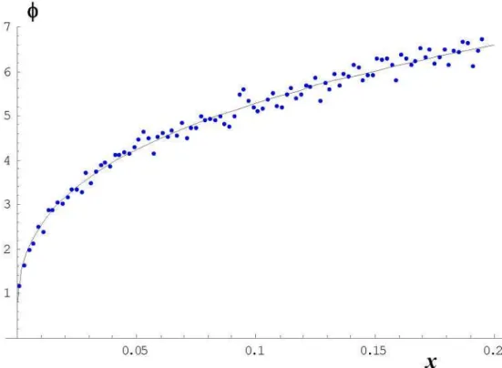
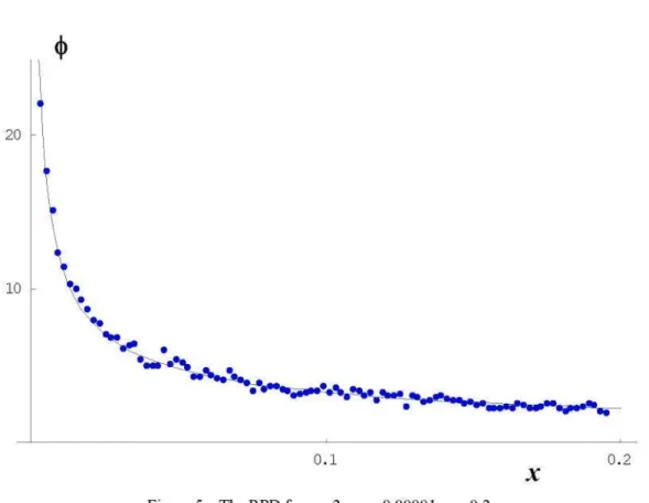
approximately constant in Fig 5b since a is close to zero.
0.05 0.1 0.15
X
0.2
Figure 5a. The RPD as a function of x for s = 0.75, e = 0.00001, c = 0.2. Dots stand for numerical results and the solid line plots the function given by Eq.(10)
6
5
4
-•
•» • _•• * - V i
0.1
X 0.2
20
10
-0.1
Figure 5c. The RPD fors = 2 , , e = 0.00001, c = 0.2.
X
0.2
3.2 Probability of the laminar length
Another important parameter for studying the intermittency phenomenon is the probability associated to the laminar length variable giving the probability of having a laminar length between / and l+dl. Following the usual method based on interpretation transposing the map local difference equation into a continuous differential equation inside the laminar region (Shuster and Just, 2005), for type-I intermittency, Eq.(l), we have
dx 2
— = e + ax
dl (11)
where / counts the number of iterations in the laminar region. After integration of the Eq.(ll) we have
/(x,c):
4ae
f
arctan
4a
A f
arctan
4a
4¿
Y
(12)
which clearly evidences that the laminar iteration number (length of the laminar region) only depends on the local map but not on the global one. Finally, the probability of finding a laminar phase length inside the interval (/; l+dl), §i(l), is given by
4>,(/) = <|>(*(/,c)) dX(l,c)
where X{l,c) is the inverse of the l(x,c) (with respect to x) extracted from Eq.(12) as
X(l, c) = —j= tan \ja arctan
yja
'a
l\jas (14)After substituting Eq.(14) into Eq.(13) the required probability is
<M0
=
a"-A sec2 (z) tana (z) ; z = arctan
v ^J
Has (15)
which for when 7 —» 0, behaves as
lim (^(7)-» Ac" (B + AC2) (16)
This last equation indicates that for a very small s, (|)/(0) is approximately constant and independent ofs,
^ ( 0 ) ~ a c2 + aA (17)
For any positive a, the function §¡(1) is a decreasing function of / , being (|)/(7)=0 when / equals the value
arctan
L
4i
yjas (18)
for a < 0, however, Eq.(18) determines the maximum laminar phase length and for I = lm the
probability of the laminar length satisfies
lim (j), (/) —» oo,
/->/, (19)
meaning that for negative a values, the laminar length l=lm isa cut-off. Having in mind the
previous relations, we can conclude that there always exists a limit value lm for /, meanwhile
the behavior of (()/(/) depends on the sign of a since for a < 0, lim (^(7) —» oo and for a > 0
lim ^ ( 7 ) ^ - 0 . /->/,
In general, the behavior of §i(l) is determined by Eq.(15) and see two relevant cases can be usefully distinguished. For a ^ O two factors govern Eq.(15), sec2(z) and tana(z), the
former is always positive whereas tana(0) = 0, furthermore, for z = 0, a limit value 7 = lm,
exists for a < 0 giving lim (^(7) —» oo and for a > 0, lim ^(7) —» 0 . For a = 0, the factor
'->'», /->/_
however in this case l = lm when z = Till
arctan
7Í
-Jas
which combined with Eq.(18) gives lim/m —» oo .
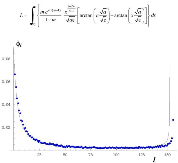
The figure Fig. 6 displays the characteristic behavior (()/(/) for positive a. Here, s = 0.6 ( a - 0 . 6 6 5 ) for both numerical (dots) and analytical results, with Eq.(15). By means of Eq.(17) we obtain (^(0) - 0.16 and from Eq.(18) we have lm = 147'. In a similar way, in Fig.
7 the typical (()/(/) behavior for negative a is presented. An excellent agreement between numerical and Eq.(15, 17 and 18) analytical results has been found again in all tested cases.
0.14 -•
0.12
0 . 1
-0.08
0.06
0.04
0.02
20 40 60 100 120 /
140
Figure 6. The probability of the laminar length for s = 0.6, e = 0.0001, a — —0.665 , c = 0.1. The solid line is obtained from Eq.(15).
3.3 Characteristic relation
The dependence of the average length of a laminar region on s is denominated the characteristic relation. The average length L can be obtained as:
with the definition of the §(x) in Eq.(lO), we get:
L =
1—2/77
mcmKm-Y) X^ T
\-m yfae
f rz\ arctan
f rz\ arctan
4a
v ^-J
> dx (21)
0.08
0.06 -I
0.04
-0.02
I:
25 50 75 100 125 150
/
Figure 7. The probability of the laminar length for s = 2, e = 0,0001, a - - 0 , 5 5 5 , c = 0.2.
To solve the integral (21), we can decompose it into two parts (here a = 1 and x¡ = 0)
^ml(m-Y) A L m c
f
L = k\ \ xa arctan f —j= \dx-
f
x arctan f41)
\dx(22)
The solution of the first integral is directly given by
a + l
/, = arctan a + l vVsy
(23)
f u = arctan x
a+l
a + 1
(24)
so that
12 = arctan
I2 = arctan
( C \ Ca+1 yfe re Xa
V s j a + l a + l-'0s +
Vsja + l a + l
-dx
(25)
If we replace the expressions for h and /2 in the L definition, we have:
L = k
a + l 3 ca+1 3 ca+1
i_ r xa+1
1+1
1 s + x
2-dx (26)
now, taking x = j-'Vs , the integral h can be written as
L=e a/2
J,
i+/)
J
(i+r)
JJ.
i + /
¿fy (27)
The second integral goes to zero as s goes to zero, the first integral converges if a is greater than -2 and less than 0, and the average laminar length is finale given by
L % S"
a +i [ 7i a
c sec
L oc e2 (28)
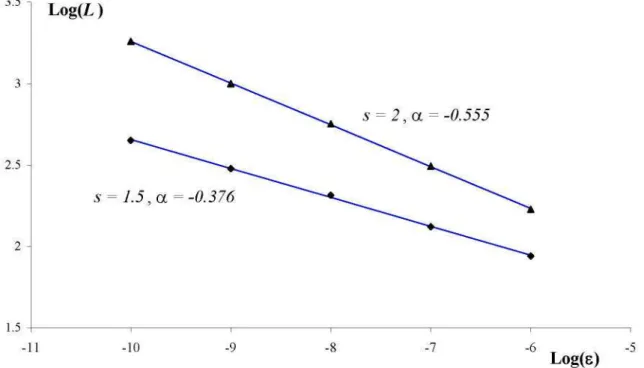
In the previous calculation we have assumed a as independent of the very small parameter s, as observed in the numerical experiments. In the Figure 8 it is shown the characteristic relation for a = -0.376 (s = 1.5) and a = -0.555 (s = 2). The numerical values (dots) are presented by the straight lines obtained by least square fitting. It can be checked that each line slope is in agreement with the value a/2 predicted by Eq.(28), as presented in following table
s
1.5 2
a/2 -0.183
-0.27
Slope in Figure 8
-0.178 -0.257
3.5
3
-2.5
2
-1.5
Log(L)
s = 1.
-ll -10 -9 -7
Log(e)
Figure 8. Characteristic relation. Marks stand for numerical data and lines correspond to least square fitting.
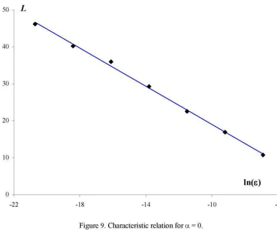
For the uniform reinjection as a particular case, a = 0, the integral h reads
L
c c X e +
x , 0.5,
ax = — I n r„2 \ - + i 0.5 A In
'iV
V J
(29)
and for small s we have
L 0.5 l n ( c2) - l n ( s ) l o c - l n ( s ) (30)
providing, as expected, the classical form of the characteristic relation, Kim et al. (1994) and Cho et al. (2002), this behavior can be seen in Figure 9 obtained for s = 1 and a - -0.03 .
50
40
30
-20
10
ln(8)
-22 -18 -14 -10
Figure 9. Characteristic relation for a = 0.
3.4 The Liapunov exponent
For any map xw+1 = f(xn), the Liapunov exponent X(x), is defined as
X(x) = lim lim l{ fN(x + 5)-fN(x) N 5
r 1 , dfN(x)
lim — l o g ^ — ^ -L (31)
where N is the number of iterations. Eq. (31) indicates that e ^ is the average factor by which the distance between closely adjacent points becomes stretched after one iteration (Schuster and Just, 2005), (5x)N = (8x)0 ew. The relation 1 A, is called the Liapunov time and
1.5
log(¿)
1.3
-1.1
0.9
-0.7
i • •
0.5
-11 -10 -7 -6
log(s)
-2
Figure 10. Characteristic relation for s = 0.75, a = 0.328. Blue marks stand for numerical results and the red ones correspond to values obtained after numerical integration of Eq.(21).
1.5 -i
1.3
1.1
-0.9
0.7
-0.5
log(¿)
: É - : : •
log(s)
-11 -10 -6 -4 -2
It is interesting to note here that log(X) is a linear function of log(s), as shown in Fig. 12 for s = 1,5 and s=2, so that we can write X <x sa. By least square method, we have checked
that the relation o * - a / 2 holds, however, this topic demands further investigations.
o i
log(X)
-0.5
1
--1.5
2
--2.5
-11
log(s)
-10
Figure 12. Liapunov exponent.
3.5 Relation between a and s
As shown in a previous paper (del Rio and Elaskar, 2009) a relation exists between the coefficient a and the exponent s (s=q in that work)
a = — - 1
s (32)
1.2 -|
a
-0.8 J
Figure 13. Relation between a and the exponent s. Marks stand for numerical results and the solid line corresponds to Eq.(32).
4 CONCLUSIONS
In this paper we have extended to the type-I intermittency phenomenon the analysis procedure we developed in a previous work in studying type-II and type-Ill intermittencies. We have found that our function M{x) is also a key tool to analyze the type-I intermittency, specially when numerical or experimental data are required in the investigation, since it is easily obtained. Therefore, M{x) is more useful and simpler than the reinjection probability density § which can be derived form the former. As a matter of fact, the reinjection probability density function, the probability of the laminar length, the average laminar length and the characteristic relation have been obtained for this case by means of numerical computations finding a good agreement with theoretical predictions. In all numerical tests we have obtained that M{x) is linear, M(x) = m x, and we have found a power law for the RPD
as §(x) = X xa which extended the usual uniform RPD, a particular case of ours for a = 0 or m
= V2. We have also verified that the relation between s and a, Eq.(32), deduced for a broad class of maps, properly holds for type-I intermittency.
Acknowledgements. This paper was supported by grants PIP - No 11220090100809 of
REFERENCES
Cho, J.; Ko, M.; Park, Y. and Kim, C , Experimental observation of the characteristic relations of type-I intermittency in the presence of noise, Physical Review E, 65: 036222. del Rio, E. and Elaskar, S., New characteristic relation for intermittency type II, International
Journal of Bifurcation and Chaos, 20 (4): 1185-1191, 2009.
del Rio, E. and Elaskar, S., Characteristic Relations and Reinjection Probability Densities (RPD) of Type-II and III Intermittencies. Effect of the noise on RPD. 8th AIMS Conference on Dynamical Systems, Differential Equations and Applications. University of Technology Dresden , Dresden, Germany, May 25 - 28, 2010.
del Rio, E.; Elaskar, S.; Donoso, J. and Conde. L., Noise influence on the Characteristic Relations and Reinjection Probability Densities of type-II and type-Ill Intermittencies. 3r
Chaos 2010 International Conference, Chania Crete Greece, 1-4 June 2010.
Elaskar, S. and del Rio, E., Reinjection Probability Function with Lower Bound of the Reinjection for Intermittency Type III. Mecánica Computadonal, 28: 1463-1476 (2009). Elaskar, S.; del Rio, E. and Donoso, J., Reinjection probability density in type-Ill
intermittency, PhysicaA. Submitted.
Kim, Ch.; Known, O.; Lee, E. and Lee, H., New characteristic relations in type-I intermittency, Physical Review Letters, 73 (4): 525-528, 1994
Kim, Ch.; Kim, G.; Kim, Y.; Kim, J. and Lee, H., Experimental evidence of characteristic relations of type-I intermittency in an electronic circuit, Physical Review E, 56 (3): 2573-2577, 1997.
Kim, M.; Lee, H.; Chil-Min Kim; Hyun-Soo Pang; Eok-Kyun Lee and Known, O., New characteristic relations in Type II and III intermittency, International Journal of Bifurcation and Chaos, 7 (4): 831-836, 1997a.
Manneville, P. and Pomeau, Y., Intermittency and the Lorenz model, Physical Letters A, 75: 1-2, 1979.
Manneville, P., Intermittency, self-similarity and \lf spectrum in dissipative dynamical systems, Le Journalde Physique, 41 (11): 1235-1243, 1980
Pomeau, Y. and Manneville, P., Intermittent transition to turbulence in dissipative dynamical systems, Communications in Mathematical. Physics, 74: 189-197, 1980.
Progogine, L, Las leyes del caos. Ed. Drakonitos, Barcelona, España, 2009.
Rusband, N., Chaotic Dynamics of Nonlinear Systems, John Wiley & Sons, New York, USA, 1990.
Schuster, H and Just, W., Deterministic Chaos. An Introduction, WILEY-VCH Verlag GmbH & Co. KGaA, Weinheim, Germany, 2005.
Won-Ho Kye and Chil-Min Kim, Characteristic relations of type-I intermittency in presence of noise, Physical Review E, 62 (5): 6304-6307, 2000.