Bayesian model selection of structural explanatory models: Application to road accident data

(1)

Procedia - Social and Behavioral Sciences 160 ( 2014 ) 55 – 63

ScienceDirect

Peer-review under responsibility of CIT 2014. doi: 10.1016/j.sbspro.2014.12.116

* Corresponding author. Tel.: +34-913-363-014; fax: +34-913-365-305.

E-mail address: [email protected]

XI Congreso de Ingenieria del Transporte (CIT 2014)

Bayesian model selection of structural explanatory models:

Application to roadaccident data

Bahar Dadashovaª*, Blanca Arenasª, José Miraª, Francisco Aparicioª

University Automobile Research Institute (INSIA), Universidad Politécnica de Madrid, José Gutiérrez Abascal 2, 28006 Madrid, Spain

Abstract

Using the Bayesian approach as the model selection criteria, the main purpose in this study is to establish a practical road accident model that can provide a better interpretation and prediction performance. For this purpose we are using a structural explanatory model with autoregressive error term. The model estimation is carried out through Bayesian inference and the best model is selected based on the goodness of fit measures. To cross validate the model estimation further prediction analysis were done. As the road safety measures the number of fatal accidents in Spain, during 2000-2011 were employed. The results of the variable selection process show that the factors explaining fatal road accidents are mainly exposure, economic factors, and surveillance and legislative measures. The model selection shows that the impact of economic factors on fatal accidents during the period under study has been higher compared to surveillance and legislative measures.

Selection and peer-review under responsibility of CIT 2014.

Keywords: Structural explanatory models; Box-Cox transformation; Bayesian inference; Markov Chain Monte Carlo; Gibbs sampling, traffic accidents; crash prediction.

1.Introduction

The main purpose in this study is to establish a practical road accident model that can provide a better interpretation and prediction performance. Structural explanatory models have proven to be very useful tool for traffic accident analysis. The models can range from simple regression model to much more sophisticated models. The main objective however remains the same i.e. is the identification of the explanatory factors that are the main © 2014 The Authors. Published by Elsevier Ltd. This is an open access article under the CC BY-NC-ND license

(2)

causes of the road accidents. The explanatory model structures have two main characteristics, the treatment of the variables through transformations, and the error structure.

In this study we are proposing a Bayesian Model Selection methodology, as the model selection strategy, where the best model from the list of candidate structural explanatory models is selected. The model structure is based on the Zellner's (1971) explanatory model with autoregressive errors. For the selection technique we are using a less parsimonious model, where the model variables are transformed using Box and Cox (1964) class of transformations. A similar approach has been carried out by Gaudry (1984), known as DRAG family models (Gaudry and Lassarre, 2000). However the model presented here differs from DRAG type of models by being less parsimonious.

A model selection strategy is proposed and the model estimation is carried out through Markov Chain Monte Carlo and Gibbs sampler. A prediction analysis is done for further cross validation. The proposed strategy allows the consecutive estimation of several models at once thus making the model estimation and selection process more efficient and less time consuming compared to DRAG models.

The rest of this chapter is organized as follows. In the first section the basic model structure is introduced. The section is followed by data description. In section 4 the methodology is proposed. In the section 5 the results of BMS and the interpretation are discussed. The section also includes the prediction analysis. The article ends with the conclusions and further work.

2.Model Structure

2.1.Structural explanatory models

The following structural explanatory model with AR(2) error term is considered (Zellner, 1971):

t l

l t l t

t k

kt k

w u u

u X Y

¦

2

U E

(1)

where ߚ௞ are the regression coefficients, ݑ௧ is an error term with the AR(2) structure and ݓ௧ are assumed to be white noise, ሺͲǡ ߪ௪ଶሻ.

We assume the power transformation of the variables included in the model. The transformation of the observations helps to achieve the normal distribution and linear growth function. The predictive accuracy has also been shown to improve substantially (Lee and Lu, 1987; Keramidas and Lee, 1990). The transformation is done as follows (Box & Cox, 1964):

0 0

) ln(

1 _z

°¯ ° ®

O O O O O

if if

Y Y Y

t t

t (2)

whereɉ௒is the transformation coefficient. In this study we propose asimpler approach to select the power transformation.For the dependent and independent variables it is limited to three values, ɉ௑ൌ ሼെͲǤͷǡͲǤͳǡͲǤͷሽ.

3.Data description

(3)

Directorate, Ministry of Public Works, National Meteorological, National Statistics Office and the Ministry of the Economy and Finance. For the Bayesian estimation process 132 observations were used. The remaining 12 observations were used to assess the prediction performance of the selected models.

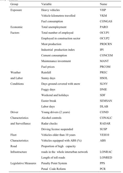
Table 1.Explanatory variables

Group Variable Name

Exposure Heavy vehicles VHP

Vehicle kilometres travelled VKM

Fuel consumption CONGAS

Economic Total unemployment PARO

Factors Total number of employed OCUP1

Employed in construction sector OCUP2

Meat production PRDCRN

Industrial production index IPI

Cement consumption CONCEM

Maintenance investment MANT

Fuel prices PRCOM

Weather Rainfall PREC

and Labor Sunny days HSOL

Conditions Days ground covered with snow SLNV

Foggy days DNIE

Weekend and holidays SDF

Easter break SEMSAN

Labor days DLAB

Driver Young drivers (2 years) COND

Characteristics Alcohol controls CONALC

and Surveillance Radar checks RADAR

Driving license suspended SUSP

Fleet Vehicles older than 10 years VEH10

Characteristics Vehicles equipped with ABS (%) ABS

Road Proportion of high capacity

Infrastructure roads in the whole interurban network LONRAC

Length of toll roads LONRED

Legislative Measures Penalty Point System PPS

Penal Code Reform PCR

4.Methodology

In this study we propose the following strategy for Bayesian model selection of structural explanatory models:

x Set the basic model structure with the autoregressive error structure and monotonic transformation values;

(4)

variables and corresponding transformation values included in the model. Select the variables that produce better goodness of fit measures;

x Estimate the models with the transformed values of the selected variables and transformed dependent variable;

x Select the candidate models with a better goodness of fit measures and right signs for the predictor, that is specified based on the substantive reasons or previous empirical studies;

x Select a single best model for the posterior prediction analysis.

4.1.MCMC

Assuming that for a given process there are K candidate models , determination of the most adequate one consists of choice of prior distributions, p(M=k) for computing the posterior model probability, p(M=k|Y=y). This procedure is referred as Bayesian Model Averaging and is implemented by using Bayes theorem. The posterior probabilities sum up to one and the best model will have the highest probability. Bayesian statisticians have derived numerous ways to evaluate and select models for inference (Gelman et al., 2004). The major limitation for the use of Bayesian approaches is the computation of the posterior distribution that requires integration of high-dimensional functions when a larger set of parameters is included in the model. However, this problem has been overcome by Markov Chain Monte Carlo (MCMC) methods which have their roots in the Metropolis algorithm (Metropolis et al., 1953) developed by physicists to compute complex integrals by expressing them as expectations for some distribution and then estimate this expectation by drawing samples from that distribution.

One particular MCMC method is the Gibbs sampler, originally developed for image processing. The Gibbs sampler is an iterative MCMC method designed to draw samples from the intractable joint distributions by sampling tractable full conditionals. See Robert and Casella (2004) for more details.

5.Results

5.1.Model estimation

The Bayesian estimation of the models begins with the assigning the prior distributions to the parameters. We are using Jeffrey's uninformative priors for the parameters. The model estimation was done using the Gibbs sampler constructed with the WinBugs software.

The first stage is the variable selection. Given the model structure and selected prior distributions, we are interested in selection of the variables that have significant effect on the response and explain the model variability best. There are originally 28 independent variables, meaning 228_{=268435456 models potentially, where each model} includes a combination of 1 to 28 variables. In order to shorten this number and simplify the estimation process, initially a set of 378 models, where each model contains combination of 2 variables were constructed.

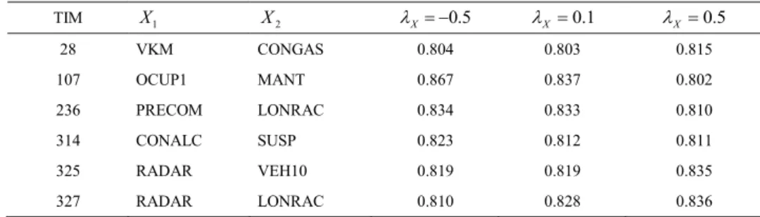
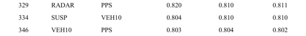
Table 2. Pseudo- ଶvalues of selected two- input models for three different values of power transformation, ɉܺ.

TIM X1 X2 OX 0.5 OX 0.1 OX 0.5

28 VKM CONGAS 0.804 0.803 0.815

107 OCUP1 MANT 0.867 0.837 0.802

236 PRECOM LONRAC 0.834 0.833 0.810

314 CONALC SUSP 0.823 0.812 0.811

325 RADAR VEH10 0.819 0.819 0.835

(5)

329 RADAR PPS 0.820 0.810 0.811

334 SUSP VEH10 0.804 0.810 0.810

346 VEH10 PPS 0.803 0.804 0.802

The variables were introduced in the model with the assigned transformation values. The transformation coefficient was limited to have three values ߣ_௫= (0.5, 0.1, 0.5). At this initial stage there was no assumption made as to which power transformation is preferred for a given variable. Thus all the variables were transformed using the same value of ߣ௫ and the set of 378 models were estimated three times, using only one value of ߣ௫. The response was not transformed. 378ή3=1134 models were visited in 2000 iterations and in three chains. Given the fact that the DIC statistics can only be compared if the data set is the same, we use pseudo R² value to see how likely the model variables explain the model.

For each value of power transformation parameter, a set of 50 models with the highest R² value were selected. The variables that appeared the most in the set of 50 models, for each value of ߣ௫, are believed to explain the model better. The results of the variable selection procedure suggest the selection of 11 variables (Table 2).

The next stage is the transformation selection for both independent and dependent variables. The transformation value for the dependent variable was obtained through the optimization process, where the non-transformed dependent and independent variables were introduced and the optimal value was selected (Venables and Ripley, 2002). The transformation value for dependent variable was set to ɉ௬ൌ ͲǤʹͷ.

Somehow the transformation selection for independent variables is not as trivial. Given the ambiguity of the variable selection process, it was not clear which power transformation value was the optimal one for a given variable, thus the ideal would be transform each variable with all three values of ߣ௫ for the model estimation, and thus determine the maximum ߣ_௫ for each variable. Considering that there are 12 variables, this would mean 3¹²=531441 potential models. To simplify this we are using DRAG model approach (Gaudry, 1984) to the transformation selection, i.e. the transformation is applied to the entire group of variables belonging to the same category rather than each variable separately. Selected 11 variables belong to 6 categories (Table 1), one of them being a legislation group with a dummy variable, meaning this variable is not subject to the power transformation. Thus, overall there are 3΁=243 variable group combinations, hence 243 models have to be estimated.

Table 3. Selected variables and the expected signs, based on previous empirical studies.

Group Variable Expected _sign

G1 VKM ൅

CONGAS ൅

G2 VEH10 ൅

G3 OCUP1 െ

MANT െ

PRECOM െ

G4 CONALC െ

RADAR െ

SUSP െ

G5 LONRAC െ

(6)

243 models were estimated using three chains taken to 10,000 iterations. The prior information for the parameters, ߠ ൌ ሼߚǡ ߩǡ ߪ௪ଶሽ are remained the same as in the first stage.

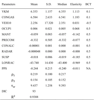
The model selection was based on the expected signs of the regressor estimates based on existing literature on road safety anddeviance information criteria- DIC (Spiegelhalter et al., 2002). Based on the previous empirical studies, a preliminary assumption on the signs of the selected variables is made (Table 3). Taking into account the estimates of the parameters, the model with better goodness of fit and matching coefficient signs were selected. Based on the DIC value, the model M=236 was selected as the best single model (DIC=93). Pseudo-R² value for this model is 0.9388, meaning more than 93% of the variability is explained (Table 4).

Table 4. Bayesian estimation of selected model, M=236.

Parameters Mean S.D. Median Elasticity BCT

VKM 6.353 1.157 6.355 1.113 0.1

CONGAS 6.584 2.633 6.541 1.183 0.1

VEH10 2.256 17.320 2.351 0.031 -0.5

OCUP1 0.006 0.021 0.005 0.068 0.5

MANT -0.059 0.083 -0.057 -0.142 0.5

PRECOM -0.332 0.505 -0.332 -0.077 0.5

CONALC -0.00001 0.001 0.000 -0.001 0.5

RADAR -0.000048 0.000 0.000 -0.008 0.5

SUSP -0.018 0.006 -0.019 -0.185 0.5

LONRAC -43.740 14.430 -43.400 -0.969 0.5

PPS -0.244 0.215 -0.240 -0.011 NA

ɏଵ 0.219 0.100 0.217

ɏଶ 0.154 0.105 0.152

ɒ௪ 9.437 1.258 9.393

DIC 93

ଶ _0.9388

In order to understand how the change in certain variables affects the response, the elasticities of the regressors were computed (Liem et al., 2008):

X Y

k kt

t k

kt t S

x X

Y Y E

X X

Y

E O

O

K 1

) ( ) (

w

w ₍₃₎

and,

kt t k

kt t S

x X

Y Y E

X X

Y E

Y

k O

K 1

) ( ) (

w

w ₍₄₎

(7)

5.2.Prediction analysis

The prediction analyses were conducted for further cross validation of BMS. For estimation 132 observations were included in the model while the remaining 12 observations were used to assess the Bayesian prediction performance. Taking into account the results of the model selection, Model 236 was used. Given the autoregressive structure of the error term, AR(2), the estimation starts after period, ൌ ͵. New observation values of dependent variables are predicted by employing the Bayesian estimates of the parameters obtained from the results of model selection. The estimation was carried out with the WinBUGS software. The Gibbs sampler was run in 10,000 iterations in 3 chains.

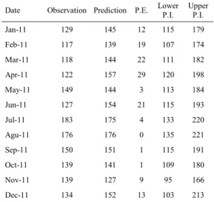
To evaluate the prediction performance of the model, 95% posterior prediction intervals were computed. As can be seen in Figure 1 all of the observations fall within the posterior prediction interval.Additionally the prediction error (Table 5) of the estimates (_௒) was computed using the following formula:

¦

T t t t Y _Y Y Y

PE 100 (5)

Table 5. Posterior prediction intervals, M=236

Date Observation Prediction P.E. Lower _P.I. Upper _P.I.

Jan-11 129 145 12 115 179

Feb-11 117 139 19 107 174

Mar-11 118 144 22 111 182

Apr-11 122 157 29 120 198

May-11 149 144 3 113 184

Jun-11 127 154 21 115 193

Jul-11 183 175 4 133 220

Agu-11 176 176 0 135 221

Sep-11 150 151 1 115 191

Oct-11 139 141 1 109 180

Nov-11 139 127 9 95 166

Dec-11 134 152 13 103 213

Figure 1. Posterior predictions, 2009- 2011

(8)

6.Discussion and further research

In this study we are considering a structural explanatory macro model for the analysis of road safety. Although these models are known to be very effective, these models are non parsimonious and thus, usual maximum likelihood estimation can be very lengthy. It has been shown that model selection based on p-values does not consider model uncertainty. Moreover, the significance of a specific parameter change is conditional on the set of the other parameters included in the model. Thus a sequential model and parameter selection can produce misleading results.

To overcome this problem we are proposing a model selection strategy using a Bayesian approach. The structural model used in the study is parsimonious. The explanatory variable selection procedure has used models with combinations of only two explanatory variables. This restriction adopted for simplicity has proved adequate in view of the results. By limiting the initial parameters (AR structure of the error term and the power transformation values) to few values, the focus on the model selection procedure is on the explanatory variable selection and BCT parameter estimation for both explanatory and response variables. The performance and improvement of the goodness of fit measures only depend on these two factors.

The results of the Bayesian estimation closely follow those obtained in previous empirical studies on road safety analysis. Moreover, the prediction analysis yields good results. The methodology has thus proved to be successful in providing a quick, simple and effective model selection strategy, which could easily be sophisticated and generalized with some additional but feasible computational cost (e.g. considering three input models in the explanatory variable selection procedure instead of just TIMs). The application to DRAG-type models provides an interesting alternative to the algorithm implemented in the TRIO software. The use of Bayesian techniques is directed to a better approximation to the true data generating process. These points will be further studied.

Acknowledgements

This work was supported by a grant from research project - TRA2011-28647-C02-01- Development of an integrated methodology for the assessment of externalities (safety and environment) for the road to rail modal shift

(MODALTRAM), from the Spanish National Research Plan 2008-2011 of the Ministry of Science and Innovation (MICINN) and was conducted at the University Institute of Automobile Research (INSIA) of the Technical University of Madrid (UPM), during 2012-2014.

References

Box, G. E., and Cox, D. R. (1964).An analysis of transformations.Journal of the Royal Statistical Society. Series B (Methodological), 26(2), 211 - 252.

Casella, G., and George, E. I. (1992).Explaining the Gibbs sampler.The American Statistician, 46(3), 167 -174.

Chib, S., and Greenberg, E. (1994). Bayes inference in regression models with ARMA (p, q) errors. Journal ofEconometrics, 64(1),183- 206. Gaudry, M. and Lassarre, S. (2000).Structural road accident models.The international DRAG family.Oxford: Elsevier Science.

Gelfand, A. E., and Smith, A. F. (1990).Sampling-based approaches to calculating marginal densities.Journal of the Americanstatistical association, 85(410), 398 - 409.

Gelman, A., Carlin, J. B., Stern, H. S., and Rubin, D. B. (2004).Bayesian data analysis.CRC.Chapman&Hall, Boca Raton,FL.

Geman, S., and Geman, D. (1984).Stochastic relaxation, Gibbs distributions, and the Bayesian restoration of images.PatternAnalysis and Machine Intelligence, IEEE Transactions on, (6), 721 - 741.

Gottardo, R., and Raftery, A. (2009). Bayesian robust transformation and variable selection: a unified approach. CanadianJournal of Statistics, 37(3), 361 - 380.

Hodges, J. S. (1987). Uncertainty, policy analysis and statistics.Statistical Science, 2(3), 259 - 275.

Keramidas, E. M., and Lee, J. C. (1990).Forecasting technological substitutions with concurrent short time series.Journal ofthe American Statistical Association, 85(411), 625 - 632.

Lee, J. C., and Lu, K. W. (1987). On a family of data-based transformed models useful in forecasting technological substitutions.Technological Forecasting and Social Change, 31 (1), 61 - 78.

(9)

Metropolis, N., Rosenbluth, A. W., Rosenbluth, M. N., Teller, A. H., and Teller, E. (1953).Equation of state calculations byfast computing machines.The journal of chemical physics, 21, 1087.

Mitra, S., and Washington, S. (2007). On the nature of over-dispersion in motor vehicle crash prediction models.AccidentAnalysis and Prevention, 39(3), 459 - 468.

Raftery, A. E. (1986).Choosing models for cross-classifications.American Sociological Review, 51(1), 145 - 146.

Regal, R. R., and Hook, E. B. (1991).The effects of model selection on confidence intervals for the size of a closed population.Statistics in Medicine, 10(5), 717 - 721.

Robert, C. P., and Casella, G. (2004).Monte Carlo statistical methods (Vol. 319).Springer, New York.

Spiegelhalter, D.J., Best, N.G., Carlin, B.P. and Van der Linde A. (2002) Bayesian Measures of Model Complexity and Fit(with Discussion).Journal of the Royal Statistical Society, Series B, 64 (4), 583 - 616.

Venables, W. N., and Ripley, B. D. (2002).Random and mixed effects. In Modern Applied Statistics WithS (271 - 300).Springer, New York. Washington, S. P., Karlaftis, M. G., and Mannering, F. L. (2011).Statistical and econometric methods for transportation dataanalysis.CRC press.

Wasserman, L. (2000).Bayesian model selection and model averaging.Journal of mathematical psychology, 44(1), 92 - 107. Zellner, A. (1971). An Introduction to Bayesian Inference in Econometrics.J. Wiley and Sons, New York.