Dynamic analysis of road vehicle-bridge systems under turbulent wind by means of Finite Element Models

(1)

Dynamic analysis of road vehicle-bridge systems under turbulent wind by means of

Finite Element Models

J. Oliva Quecedo1_{, P. Antolín Sánchez}1_{, J. M. Goicolea}1_{, M. Á. Astiz}1 1_{Department of Mechanics and Structures, School of Civil Engineering,} Technical University of Madrid, Profesor Aranguren s/n 28040, Madrid, Spain

email: joliva@mecanica.upm.es,pantolin@mecanica.upm.es,goicolea@mecanica.upm.es,miguel.a.astiz@upm.es

ABSTRACT: When an automobile passes over a bridge dynamic effects are produced in vehicle and structure. In addition, the bridge itself moves when exposed to the wind inducing dynamic effects on the vehicle that have to be considered. The main objective of this work is to understand the influence of the different parameters concerning the vehicle, the bridge, the road roughness or the wind in the comfort and safety of the vehicles when crossing bridges. Non linear finite element models are used for structures and multibody dynamic models are employed for vehicles. The interaction between the vehicle and the bridge is considered by contact methods. Road roughness is described by the power spectral density (PSD) proposed by the ISO 8608. To consider that the profiles under right and left wheels are different but not independent, the hypotheses of homogeneity and isotropy are assumed. To generate the wind velocity history along the road the Sandia method is employed. The global problem is solved by means of the finite element method. First the methodology for modelling the interaction is verified in a benchmark. Following, the case of a vehicle running along a rigid road and subjected to the action of the turbulent wind is analyzed and the road roughness is incorporated in a following step. Finally the flexibility of the bridge is added to the model by making the vehicle run over the structure. The application of this methodology will allow to understand the influence of the different parameters in the comfort and safety of road vehicles crossing wind exposed bridges. Those results will help to recommend measures to make the traffic over bridges more reliable without affecting the structural integrity of the viaduct.

KEY WORDS: Road vehicle dynamics; Road roughness; Turbulent cross wind; Dynamic interaction; Bridges; Passenger comfort

1 INTRODUCTION

Cars, high-sided vehicles and heavy trucks are exposed to risks on locations where topographical features magnify the wind effects such as embankments and bridges. Moreover, when an automobile passes over a bridge dynamic effects are produced in vehicle and structure. Those dynamic effects not only magnify the forces in the bridge, but also affect the comfort and safety of the traffic. In addition, the bridge itself moves when exposed to the wind inducing dynamic effects on the vehicle that have to be considered. Thus, comfort and safety of the traffic over viaducts may be jeopardized when cross-wind is blowing. Recent work in this field has focused on long span cable-stayed or suspension bridges ([1], [2], [3], [4], [5]). But more conventional bridges can also be affected by high speed cross-winds, for example continuous approach viaducts.

Besides the cross-wind action, the road roughness is also an important source of dynamic excitation that has to be considered. Some previous works in this field have neglected the differences in the road profile under the left and the right wheels, that differences are in this work taken into account by assuming that the road surface is homogeneous and isotropic ([6], [7]).

In section 2 vehicle, bridge and interaction models are described. The methodology for reproducing the interaction between the vehicle and the bridge is verified with two benchmarks ([8], [9]). In sections 3 and 4 the methods for computing the road profiles and the wind velocity fields are

explained. In section 5 results are presented and concluding remarks are reported in section 6.

The understanding of the influence that the different elements have in this dynamic problem will help in the task of recommending measures to make the traffic over bridges more reliable without affecting the structural integrity of the viaduct.

2 VEHICLE AND BRIDGE MODELS

The vehicle is modeled as a combination of rigid solids with masses and rotary inertias connected by springs and dampers which represent the dynamic properties of suspensions and tyres. The vehicle proposed by Coleman and Baker [10] that has been employed by other authors ([2], [5], [11]) is used in this work. It is intented to represent high-sided vehicles that are sensitive to the cross winds.

(2)

(a)

(b)

Figure 1. Vehicle model: (a) Side view; (b) Rear view.

the model has a total of eleven DOF and includes, not only the vertical behavior, but also the lateral one, which is necessary for the analysis under turbulent cross winds. Figure 1 shows a sketch of the model and table 1 summarizes its mechanical properties. The eigenmodes of the vehicle model are reported in table 2.

In regard to structures, previous work has focused mainly in long span cable-stayed or suspension bridges. But problems could also appear in more conventional bridges with shorter spans where the wind velocity could also be high. As for example in deep valleys or in approach viaducts of long bridges. In this study a concrete-steel composite five-span continuous bridge is analysed. The cross section is a 25 meters wide box girder. The total length of the viaduct is 220 meters distributed in five spans of 40, 45, 50, 45 and 40 meters. The road over the bridge has two lanes per direction, the vehicle runs in the outer lane.

Three dimensional Timoshenko beam elements are employed to model the deck by means of the finite element method. Rayleigh structural damping is assumed. The mechanical properties of the bridge are not constant over its length, in table 3 some characteristics of the central cross section of the main span are given. Table 4 reports the six first eigenmodes of the bridge.

The whole problem is solved by the Finite Element Method in a fully coupled system. The interaction is reproduced by a linear penalty method between the lower nodes of the vehicle and the bridge surface. The contact between the bridge deck and each tyre is assumed to be a point contact and there is no sliding. The assumption that the tyres have to be in contact with the bridge surface is not adopted here, so each tyre can separate from the surface. Dynamics equations are solved by direct integration in time using the HHT method [12]. In order to verify this methodology two benchmarks have been used ([8], [9]). Results are in very good agreement, but they are not reported here for the sake of brevity.

3 ROAD ROUGHNESS

The road profile irregularities can be represented with a normal stationary ergodic random process described by its Power Spectral Density (PSD). Several PSD functions have been proposed by different authors (e.g. [6], [13]). A survey of different approximations can be found in Andrén [14]. ISO 8608 [15] specifications propose a distribution for the one-sided PSD defined by the following expression:

G(n) =G(n0) _n

n0

−2

(1)

where G(n) is the one-sided power spectral density for the spatial frequencyn andG(n0)is the one-sided power spectral density for the reference spatial frequency or wavenumbern0= 0.1 m−1_{. The value for}_G₍_n₀₎_{is prescribed by ISO 8608 [15] as} a function of the road class. The road profile is generated as the sum of a series of harmonics:

yl(x) = Nn

∑

i

p

2G(ni)∆ncos(2πnix+φi) (2)

whereφiis the random phase angle uniformly distributed from 0 to 2π. This expression employsNnspatial frequencies between two values, nmin and nmax. Thus the increment value (∆n) is constant:

∆n=nmax−nmin

Nn (3)

(3)

Table 1. Vehicle mechanical properties.

Stiffnesses [N/m]

Element Notation Value

All tyres (vertical) ky,ti(i=1,2,3,4) 3.51·105 All tyres (lateral) kz,ti(i=1,2,3,4) 1.21·105 All suspensions (vertical) ky,si(i=1,2,3,4) 3.99·105 All suspensions (lateral) kz,si(i=1,2,3,4) 2.99·105

Dampings [N_·s/m]

All tyres (vertical) cy,ti(i=1,2,3,4) 800.0 All tyres (lateral) cz,ti(i=1,2,3,4) 800.0 Rear suspensions (vertical) cy,s1,cy,s2 5180.0 Rear suspensions (lateral) cz,s1,cz,s2 5180.0 Front suspensions (vertical) cy,s3,cy,s4 23210.0 Front suspensions (lateral) cz,s3,cz,s4 23210.0

Masses [kg]

Rear wheels mt1,mt2 710.0

Front wheels mt3,mt4 800.0

Body mb 4480

Rotary inertias [kg·m2_]

Body (roll) Iα,b 1349.0

Body (yaw) Iβ,b 1.0·105

Body (pitch) Iγ,b 5516.0

Table 2. Vehicle eigenmodes and eigenfrequencies. Mode Number Main body DOF Frequency [Hz]

1 z+β+α 0.98

2 z+α+β 1.18

3 y+γ 1.81

4 α+z 2.56

5 γ 3.29

6 α+β 4.17

7 α+z 4.70

8 α 5.05

9 y+γ 5.45

10 α+z 8.22

11 γ 11.85

The enveloping effect of the tyre acts as a low-pass filter for the road vibration input to the vehicle. The short wavelengths, or the high spatial frequencies are not taken into consideration. The filter effect depends on the size and construction of the tyre. For general on-road cases this results in a lower limit for the

Table 3. Bridge properties.

Parameter Unit Value

Cross-sectional area m2 ₀_.₉₆₄

Cross-sectional vertical inertia m4 ₀_.₆₃₈ Cross-sectional transversal inertia m4 ₃₃_.₆₇₅ Cross-sectional torsion inertia m4 ₁_.₅₇₁

Non structural mass kg/m 11543.0

Elastic modulus N/m2 ₂_.₁_·₁₀11

Table 4. Bridge eigenmodes and eigenfrequencies.

Mode Number Type Frequency [Hz]

1 Vertical bending 1.82

6 Torsion 4.12

wavelengthλ=0.1 m [15]; that is, an upper limit for the spatial frequencies ofnmax=10.0 m−1.

For the sake of shortness, comparison of generated random profiles and target spectral densities was not included here. Those results were in excellent agreement.

Kropac and Mucka [16] propose a relation between the International Roughness Index, IRI ([17], [18]), and the PSD. For the definition proposed in ISO 8608 that relation results in:

IRI=2.21 r

G(n0)

16 (4)

Thus, we can obtain the IRI for each road class defined in the ISO 8608 specifications or inversely obtain the value ofG(n0) to have a preset value for the IRI.

A surface description complete enough to define the profiles under left and right tyres is needed. Making provision for the different excitation at the two sides of a vehicle complicates the problem. It is necessary to provide descriptions of a pair of profiles for each case instead of only one, and this requires the specification of the two direct spectral densities and the two cross-spectral densities. An alternative is to describe the surface through a two-dimensional spectral density, a function of two wavenumbers. This process would be very long-lasting and laborious both in data acquisition and computation. If the hypothesis of homogeneity and isotropy is accepted the surface description is simplified and the cross-spectral densisty can be obtained from the direct spectral density ([6], [19], [9]).

In a homogeneous and isotropic surface every straight profile has the same statistical characteristics, independently from its direction or position. If we consider two parallel profiles (left and right), their autocorrelation functions will be identical and the cross-correlation functions are also the same:

Rl(δ) =Rr(δ) =R(δ) Rlr(δ) =Rrl(δ) =Rx(δ) (5) It can be easily demonstrated ([6], [7]) that:

Rx(δ) =R(

q

(4)

0 0.1 0.2 0.3 0.4 0.5 0.6 0.7 0.8 0.9 1

0.01 0.1 1 10

Coherency

Spatial frequency [m−1]

Figure 2. Coherency for vehicle width (2.20 m).

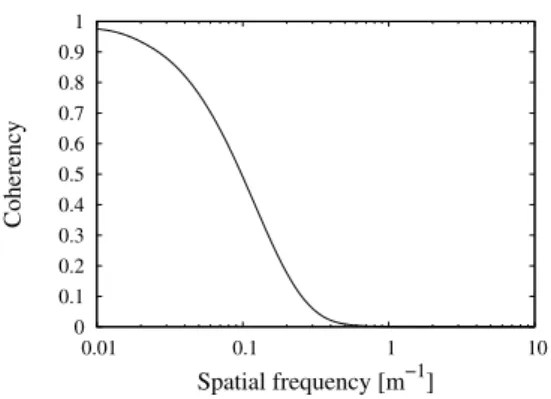
AndGxcan be obtained by means of the Fourier Transform. The two profiles direct spectral densities will be the same (Gl(n) = Gr(n) = G(n)) and so are the two cross-spectral densities (Grl(n) = Glr(n) = Gx(n)). Thus, the coherency function is defined as follows [19]:

g(n) =|Gx(n)|

G(n) (7)

In Figure 2 coherency for two profiles at a distance of 2.20 m, that is the vehicle width, is graphed and figure 3 shows left and right profiles at a distance equal to 2.20 m with IRI=2.0 dm/hm.

−15 −10 −5 0 5 10 15

0 20 40 60 80 100

Elevation (mm)

Distance (m)

Left track Right track

Figure 3. Parallel profiles at a distance of 2.20 m.

4 WIND SPEED

Turbulent wind velocity history in one point can be represented with a normal stationary ergodic random process. In the same way as the road roghness, it can de described by its Power Spectral Density and the time history is generated as the sum of a series of harmonics with frequencies in the range[0,fmax]. That range is divided in bands of equal width (∆f). Thus, a total of Nf = f_∆max_f frequencies are considered. For example for the longitudinal componentu(t):

u(t) = Nf

∑

i=1 p

2Gu(fi)∆fcos(2πfit+θi) (8)

where Gu(fi) is the one-sided PSD for fi =i·∆f, θi is the random phase angle uniformly distributed from 0 to 2π. v(t)

andw(t) can be computed in the same way. When not only the time-history of one turbulent wind component is needed it is usual to neglect the relation between the different components, mainly when the distance to the ground is high enough, as for example in bridge decks ([20],[21]). A spectral definition for the three components is needed. Kaimal spectrum [22] is commonly adopted and is the one proposed by the Eurocode [23]. An auto-spectrum is given for each one of the three components:

f·Gn(f)

σ2

n =

Anfˆn 1+1.5Anfˆn5/3

n=u,v,w (9)

wheref is the frequency,Gnare the one-sided PSDs,σnare the standard deviations, ˆfn means adimensional frequency andAn are constants.

To simulate time histories of the wind velocity at several points in space it must be taken into consideration that they are not independent. This dependency is related to the distance between points, the closer are the points the higher is the coherence, and also to the frequency, coherence is higher for lower frequencies as it is related to bigger eddies.

The bridge deck is assumed to be horizontal and at a constant distance from the ground so that the mean wind velocity is constant over the bridge length. Horizontal homogeneity is assumed so that the statistical properties of the wind field are the same in the whole deck. Coherence function is then defined as:

γn=e−Cn f dU n=u,v,w (10)

where f is the frequency,d is the distance between the points,

Uis the mean wind speed andCnare decay coefficients that are assumed to be constant.

Veers ([24], [25]) presents a methodology to compute wind velocity fields from a PSD and a coherence function, it is named Sandia after theSandia National Laboratories(USA), where it was developed. Cao [21] proposed some simplifications that make the computation faster. In this paper Sandia method is employed as the computation time is not considered critical. A good explanation of the method can be found in [26].

4.1 Wind forces on vehicle

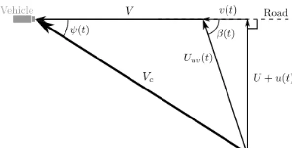
The mean wind velocity (U) is supposed to be perpendicular to the bridge axis, that is to say, perpendicular to the road. Thus the turbulent componentvis aligned with the vehicle speed. The horizontal wind velocity at a single point is the composition of

U,u(t)andv(t)(figure 4), and will be hereinafter calledUuv. If

vis considered, the angle between the horizontal wind and the road will be no longer constant and equal to 90o_{, that angle will} be calledβ and varies with time.

To obtain the wind velocity relative to the vehicle and the attack angle the running speed has to be considered (figure 4) and they can be expressed as:

Vc(t) =

q

[V+Uuv(t)cos(β(t))]2+ [Uuv(t)sin(β(t))]2 (11)

ψ(t) =arctan

_U

uv(t)sin(β(t))

V+Uuv(t)cos(β(t))

(12)

(5)

Figure 4. Relative wind velocity in the vehicle.

the vehicle is between two of those points the wind velocity has to be interpolated. The quasi-static aerodynamic forces and moments are computed as:

FN=1

2ρVc2CN(ψ)Af N=D,L,S (13a)

MN=1₂ρVc2CN(ψ)Afhv N=R,Y,P (13b)

whereD,LandSare for drag, lift and side forces; R,Y andP

are for roll, yaw and pitch moments respectively; ρ is the air density; Af is the reference area of the vehicle andhv is the reference height, that is normally taken as the vertical distance from the vehicle centre of gravity to the ground.

The set of coefficients proposed by Snæbjörnsson [11] for a high-sided vehicle show a good agreement with full-scale measurements, wind tunnel tests and CFD simulations reported in the literature [27] and have the advantage of being a complete set with information regarding every force and moment:

CD(ψ) =−0.5(1+sin(3ψ)) (14a)

CL(ψ) =0.75(1.5−0.9cos(4ψ)−0.6cos(2ψ)) (14b)

CS(ψ) =−5.5sin(ψ) (14c)

CR(ψ) =₋2.2sin(ψ) (14d)

CP(ψ) =₋7.2sin2(ψ) (14e)

CY(ψ) =cos(4ψ)−1.0 (14f)

these coefficients are defined with respect to the centre of gravity of the truck body.

4.2 Wind forces on bridge

The mean wind speed (U) is horizontal and perpendicular to the deck. The componentu is horizontal as well andwis vertical and perpendicular to the bridge deck. Thus an angle α(t) is formed by the horizontal and the total wind speed.vis neglected when computing the effects on the bridge. Self-excited forces in the bridge are not considered as the wind speed is low and the displacements of the deck are small.

The drag and lift forces and the overturning moment in the deck can be computed:

FD=1₂ρUuw2CD(α)A (15a)

FL=1

2ρUuw2CL(α)B (15b)

MO=1₂ρUuw2CO(α)B2 (15c)

Figure 5. Wind velocity in the deck.

whereA is the depth of the bridge cross section andB is its width, coefficientsC(α)are those reported by Strømmen [20].

5 RESULTS

In this section results obtained with the models and methods described before are presented. First, dynamic behaviour of the vehicle running along a rigid road is analyzed. Afterwards the bridge is added to the model.

5.1 Vehicle running along a road

Wind velocity time histories are computed for one kilometer of straight road. Turbulence intensity in the longitudinal component (Iu) is set as 14 %. The other turbulence intensities are assumed to beIv=0.75IuandIw=0.50Iu([20], [28], [29]). Mean wind speeds of 5, 10, 15, 17, 20, 22 , 25 and 30 m/s have been considered. For each value ofU five time histories are calculated in order to improve the statistical significance. The vehicle runs along that windy stretch at different speeds (10, 30, 50, 70, 90, 110 km/h).

Two stability criteria are used in this work by means of accident indices, rollover and side slip. Rollover accident index considers the load transfer between vehicle sides. When there is no load transfer the index is 0.0; when it is about to overturn, that is, when the force at one side is null, the value is 1.0. This index is defined as:

ηrollover=F_Fy,le f t−Fy,right

y,le f t+Fy,right <1.0 (16)

whereFy,le f tandFy,right are the vertical reaction at leeward and windward tyres respectively, wind comes from the right of the vehicle.

Due to the cross wind windward wheels are unloaded, if the vertical load that the windward tyre transfer to the pavement decreases the point when the horizontal load is higher that the horizontal resistance may be reached and the tyre will only bear a horizontal force equal toµFy, whereµ is the frictional coefficient andFyis the vertical load. The rest of the horizontal force has to be resisted by the leeward tyre. Thus the stability criterion for lateral slip is set in that wheel:

ηsideslip=Fz,le f t+F_µFz,right−µFy,right

y,le f t <1.0 (17)

whereFzmeans lateral force.

(6)

0 5 10 15 20 25 30 35

10 30 50 70 90 110

U [m/s]

V [km/h] unsafe

safe

Dry asphalt Wet asphalt

Figure 6. CWC in a rigid road without roughness.

can be defined. That curves are graphed in figure 6 for dry asphalt (µ=0.9) and for wet asphalt (µ=0.5).

Figures 11 and 12 show the root mean square of the vertical and lateral acceleration for safeU-V pairs in dry asphalt and for

U equal to 5, 10, 15 and 20 m/s. IfU=20 m/s the maximum vehicle speedV is 70 km/h. Lateral acceleration is higher than vertical. Figure 9 represents the mean value of the minimum vertical load at the windward rear tyre, which is the more prone to lift; it is the mean value of the five wind histories considered.

0 0.1 0.2 0.3 0.4 0.5 0.6 0.7

10 30 50 70 90 110

Vertical acceleration [m/s

2]

Vehicle speed [km/h] U=5 m/s

U=10 m/s U=15 m/s U=20 m/s

Figure 7. Vehicle vertical acceleration RMS in a rigid road without roughness.

0 0.1 0.2 0.3 0.4 0.5 0.6 0.7

10 30 50 70 90 110

Lateral acceleration [m/s

2]

U=10 m/s U=15 m/s U=20 m/s

Figure 8. Vehicle lateral acceleration RMS in a rigid road without roughness.

The effect of the road roughness is now added to the model. The road profiles have been created by setting an IRI equal to 2.0 dm/hm. Ten different one kilometer long profiles have been generated and have been combined with the five wind histories, as a result we have 50 cases for each pairU-V. The

0 2000 4000 6000 8000 10000 12000 14000 16000 18000 20000

10 30 50 70 90 110

Minimum vertical reaction T2 [N]

U=10 m/s U=15 m/s U=20 m/s

Figure 9. Minimum vertical load under rear windward tyre in a rigid road without roughness.

new Critical Wind Curves are graphed in figure 10. The RMS of vertical and lateral accelerations considering both the cross wind and the irregularities are shown in figures 11 and 12. Lateral acceleration is almost the same that in the previous case, showing that the wind is the dominant factor. Vertical acceleration gets increased and the curves for different values of

U are closer showing that, with this level of irregularities, road roughness is dominant regarding vertical acceleration. A peak can be appreciated between 50 and 70 km/h, that happens due to the fact that a resonant effect appears in the vehicle because the third vehicle mode is excited by the road roughness. The minimum vertical load at windward rear tyre is shown in figure 13. It can be seen that the pairU=20 m/s -V=70 km/h is not safe.

0 5 10 15 20 25 30 35

10 30 50 70 90 110

U [m/s]

V [km/h] unsafe

safe

Dry asphalt Wet asphalt

Figure 10. CWC in a rigid road with roughness (IRI=2.0 dm/hm).

5.2 Vehicle running over a bridge

(7)

0 0.1 0.2 0.3 0.4 0.5 0.6 0.7

10 30 50 70 90 110

2]

U=10 m/s U=15 m/s U=20 m/s

Figure 11. Vehicle vertical acceleration RMS in a rigid road with roughness (IRI=2.0 dm/hm).

0 0.1 0.2 0.3 0.4 0.5 0.6 0.7

10 30 50 70 90 110

Lateral acceleration [m/s

2]

U=10 m/s U=15 m/s U=20 m/s

Figure 12. Vehicle latercal acceleration RMS in a rigid road with roughness (IRI=2.0 dm/hm).

0 2000 4000 6000 8000 10000 12000 14000 16000 18000 20000

10 30 50 70 90 110

Minimum vertical reaction T2 [N]

U=10 m/s U=15 m/s U=20 m/s

Figure 13. Minimum vertical load under rear windward tyre in a rigid road with roughness (IRI=2.0 dm/hm).

on the windward rear tyre when V is 70 km/h, the vertical reaction is almost the same. So we can conclude that the bridge affects mainly to the comfort not to the safety. In figure 16 the RMS of the vertical acceleration for U=20 m/s at different vehicle speeds is graphed. If road roughness is considered the differences in the vertical acceleration RMS decrease (figure 17).

6 CONCLUSIONS

In this work a vehicle and a bridge have been modeled and its interaction has been reproduced by means of finite element models with a linear penalty contact model. Road roughness is computed from the Power Spectral Density proposed in the ISO 8608 specifications [15], isotropy and homogeneity hypotheses

−1.5 −1 −0.5 0 0.5 1 1.5

0 20 40 60 80 100 120 140 160 180 200 220

2]

Distance [m] Bridge

Ground

Figure 14. Vertical acceleration in the vehicle on the bridge and on the road (U=20 m/s -V=50 km/h).

0 1000 2000 3000 4000 5000 6000 7000 8000 9000

0 20 40 60 80 100 120 140 160 180 200 220

Vertical load [N]

Distance [m] Bridge

Ground

Figure 15. Vertical reaction in the windward rear wheel on the bridge and on the road (U=20 m/s -V=70 km/h).

0 0.1 0.2 0.3 0.4 0.5

10 30 50 70

Vertical acceleration RMS [m/s

2]

V [km/h] Bridge

Ground

Figure 16. RMS of vertical acceleration without road roughness on the bridge and on the road.

are assumed for considering the road profiles under left and right tyres. Wind speed in different points is computed by the Sandia method [25]. Those actions are applied first to the vehicle alone and afterwards to the vehicle running over a five-span bridge. We can come to several conclusions after the application of the models and methods described before.

Finite Element Models with linear penalty method are suitable for taking into account the vehicle-structure interaction in this kind of problems.

Eigenfrequencies of the vehicle have been computed, they are located approximately between 1 and 10 Hz. The first eigenfrequency of the bridge is 1.82 Hz.

(8)

0 0.1 0.2 0.3 0.4 0.5

10 30 50 70

Vertical acceleration RMS [m/s

2]

V [km/h] Bridge

Ground

Figure 17. RMS of vertical acceleration with road roughness (IRI=2.0 dm/hm) on the bridge and on the road.

than 22 m/s safety is jeopardized. We have to keep in mind that those CWC have been calculated with a turbulence intensity

Iu of 14 %. CWC are more restrictive when the pavement is wet because side slip is more likely to happen. The critical mean wind speed is then approximately 5 m/s lower than in dry asphalt.

When road roughness is considered CWC are also more restrictive because irregularities induce vertical excitation of the vehicle and reduce the vertical loads under tyres. The road profiles considered have an IRI equal to 2.0 dm/hm.

Windward rear wheel is the most prone to initiate the overturning accident. The side slip scenario is most likely to take place at the rear axle also.

When road roughness is taken into consideration a resonant effect appears when the vehicle speed is between 50 and 70 km/h, that happens because the third vehicle eigenmode is excited by the road.

Cross winds induce higher lateral accelerations than vertical. When road irregularities are included the lateral acceleration remains almost the same, but vertical acceleration gets higher. That vertical acceleration is almost independent of the wind speed, it is due to the fact that vertical effects of road profiles with an IRI equal to 2.0 dm/hm are more important that those coming from the wind at 20 m/s.

The lateral effects of the presence of the bridge are negligible. But its vertical movement due to the wind induces high vertical accelerations in the vehicle affecting the passengers comfort. The influence on the vertical load under the tyres is lower so the effect on safety seems to be lower.

When the road roughness is included in the vehicle-bridge-wind problem bridge influence decreases because the irregularities become dominant. It is important to remark that we have used profiles with IRI equal to 2.0 dm/hm. If the IRI of the road is lower the influence of the bridge would be higher.

REFERENCES

[1] C. S. Cai and S. R. Chen, “Framework of vehicle-bridge-wind dynamic analysis,”Journal of Wind Engineering and Industrial Aerodynamics, vol. 92, pp. 579–607, 2004.

[2] S. R. Chen and C. S. Cai, “Accident assessment of vehicles on long-span bridges in windy environments,” Journal of Wind Engineering and Industrial Aerodynamics, vol. 92, pp. 991–1024, 2004.

[3] Y. L. Xu and W. H. Guo, “Dynamic analysis coupled road vehcile and cable-stayed bridge systems under turbulent wind,” Engineering Structures, vol. 25, pp. 473–486, 2003.

[4] Y. L. Xu and W. H. Guo, “Effects of bridge motion and crosswind on ride comfort of road vehicles,” Journal of Wind Engineering and Industrial Aerodynamics, vol. 92, pp. 641–662, 2004.

[5] W. H. Guo and Y. L. Xu, “Safety analysis of moving road vehicles on a long bridge under crosswind,” Journal of Engineering Mechanics, vol. 132 (4), pp. 438–446, 2006.

[6] C. J. Dodds and J. D. Robson, “The description of road surface roughness,” Journal of Sound and Vibration, vol. 31, pp. 175–183, 1973.

[7] K. M. A. Kamash and J. D. Robson, “The application of isotropy in road surface modelling,”Journal of Sound and Vibration, vol. 57, pp. 89–100, 1978.

[8] Yeong-Bin Yang and Jong-Dar Yau, “Vehicle-bridge interaction element for dynamic analysis,” Journal of Structural Engineering, vol. 123 (11), pp. 1512–1518, 1997.

[9] S. Marchesiello, A. Fasana, L. Garibaldi, and B. A. D. Piombo, “Dynamics of multi-span continuous straight bridges subject to multi-degrees of freedom moving vehicle excitation,”Journal of Sound and Vibration, vol. 224, pp. 541–561, 1999.

[10] S. A. Coleman and C. J. Baker, “High sided road vehicles in cross winds,” Journal of Wind Engineering and Industrial Aerodynamics, vol. 36, pp. 1383–1392, 1990.

[11] J. Th. Snæbjörnsson, C. J. Baker, and R. Sigbjörnsson, “Probabilistic assessment of road vehicle safety in windy environments,” Journal of Wind Engineering and Industrial Aerodynamics, vol. 95, pp. 1445–1462, 2007.

[12] H. M. Hilber, T. J. R. Hughes, and R. L. T. Taylor, “Improved numerical dissipation for time integration algorithms in structural dynamics,” Earthquake Engineering and Structural Dynamics, vol. 5, pp. 283–292, 1977.

[13] H. Honda, Y. Kajikawa, and T. Kobori, “Spectra of road surface roughness on bridges,” Journal of the Structural Division (ASCE), vol. 116, pp. 1036–1051, 1982.

[14] P. Andrén, “Power spectral density aproximations of longitudinal road profiles,”Int. J. Vehicle Design, vol. 40, pp. 2–14, 2006.

[15] ISO-8608, “Mechanical vibration - Road surface profiles - Reporting of measured data,” 1995.

[16] O. Kropac and P. Mucka, “Effects of longitudinal road waviness on vehicle vibration response,”Vehicle System Dynamics, vol. 47, pp. 135–153, 2009. [17] M. W. Sayers, T. D. Gillespie, and W. D. Paterson, “Guidelines for conducting and calibrating road roughness measurements,” Tech. Rep. 46, Banco Mundial, 1986.

[18] M. W. Sayers, T. D. Gillespie, and C. Queiroz, “The international road roughness experiment: Establishing correlation and a calibration standard for measurements,” Tech. Rep. 45, Banco Mundial, 1986.

[19] K. M. A. Kamash and J. D. Robson, “Implications of isotropy in random surfaces,”Journal of Sound and Vibration, vol. 54, pp. 131–145, 1977. [20] Einar N. Strømmen, Theory of Bridge Aerodynamics, Springer, Berlin,

Germany, 1st edition, 2006.

[21] Y. Cao, H. Xiang, and Y. Zhou, “Simulation of stochastic wind velocity field on long-span bridges,”Journal of Engineering Mechanics, vol. 126, 2000.

[22] J. C. Kaimal, J. C. Wyngaard, Y. Izumi, and O. R. Coté, “Spectral characteristics of surface-layer turbulence,” Journal of the Royal Meteorological Society, vol. 98, pp. 563–589, 1972.

[23] EN1991-1-4, “Eurocode 1: Actions on structures - Part 1-4: General actions. Wind actions,” European Committee for standardization (CEN), 2005.

[24] Paul S. Veers, “Modeling stochastic wind loads on vertical axis wind turbines,” Tech. Rep. UC-60, Sandia National Laboratories, 1984. [25] Paul S. Veers, “Three-dimensional wind simulation,” Tech. Rep. UC-261,

Sandia National Laboratories, 1988.

[26] Martin O. L. Hansen,Aerodynamics of Wind Turbines, Earthscan, London, UK, 2nd edition, 2008.

[27] M. Sterling, A. Quinn, D. Hargreaves, F. Cheli, E. Sabbioni, G. Tomasini, D. Delaunay, C. Baker, and H. Morvan, “A comparison of different methods to evaluate the wind induced forces on a high sided lorry,” Journal of Wind Engineering and Industrial Aerodynamics, vol. 98, pp. 10–20, 2010.

[28] Claës Dyrbye and Svend O. Hansen,Wind loads on Structures, John Wiley & Sons, Chichester, UK, 1999.