Weakly Nonlinear Oscillations of Nearly Inviscid Axisymmetric Liquid Briges

Weakly nonlinear oscillations of nearly inviscid

axisymmetric liquid bridges

By J O S É A. N I C O L Á S A N D J O S É M. V E G A ETSI Aeronáuticos, Universidad Politécnica de Madrid, 28040-Madrid, Spain

{Received 9 August 1995 and in revised form 22 May 1996)

A weakly nonlinear analysis is presented of the small oscillations of nearly inviscid . liquid bridges subjected to almost resonant axial vibrations of the disks. An amplitude equation is derived for the evolution of the complex amplitude of the oscillations that exhibits hysteresis and period doublings. We also analyse the steady streaming in the bulk forced by the oscillatory boundary layers near the disks; the boundary layer near the free surface produces no forcing terms. In particular some experimentally observed patterns are explained, and some new, non-observed ones are predicted. We conclude that the structure of this steady flow is not the appropriate one to counterbalance steady thermocapillary convection, but our results indícate how to get the desired counterbalancing eífect.

1. Introduction

The stability and dynamics of liquid columns and jets were considered in the pioneering work by Plateau (1849, 1863) and Rayleigh (1879, 1892), after the earlier basic analyses on capillary interfaces by Young (1805) and Laplace (1805). In the last twenty years the interest in these configurations has increased due to their applications in some industrial processes and natural phenomena. In particular, liquid bridges are of interest in materiaís processing (Preiser, Schwabe & Sharman 1983; Kamotani, Ostrach & Vargas 1984; Brown 1988) and have been observed in flow through porous media (Melrose 1966; Zasadzinski et al. 1987) and particulates agglomeration (Chen, Tsamopoulos & Good 1992); other applications include the experimental measurement of viscosity and surface tensión (Tsamopoulos, Chen & Borkar 1992), and their use as accelerometers.

used by Borkar & Tsamopoulos (1991) to calcúlate a first correction to the natural frequencies and a first approximatíon of the damping rates, that only accounted for viscous dissipation in the Stokes boundary layers near the disks supporting the bridge. Unfortunately, although these results are asymptotically correct, they provide a poor approximatíon to the damping rate, except for unrealistically large valúes of the capillary Reynolds number, as shown by Higuera, Nicolás & Vega (1994), who calculated a second approximatíon (accounting for viscous dissipation both in the Stokes boundary layers and in the bulk) to obtain quite good results for moderately large Reynolds numbers; see also Nicolás & Vega (1996) for a comparison with almost exact results obtained by a semi-analytical method that allows cheap computations for arbitrary valúes of the capillary Reynolds number.

The only theoretical work in the literature concerning nonlinear mechanicaí oscií-lations of non-inviscid liquíd bridges, not using one-dimensional approximations, is a recent paper by Chen & Tsamopoulos (1993), who analysed fully nonlinear oscií-lations by direct numerical simulation. They considered only moderately large valúes of the capillary Reynolds number, C1 ^ 50; their computations are seemingly too

expensive for larger valúes of C~l. They showed in particular how nonlinear terms

affect quantitatively the natural frequencies and damping rates.

In this paper we consider the weakly nonlinear response of an axisyrnmetric, nearly inviscid liquid bridge to forced vibrations of the disks, of appropriately smaíl ampli-tude and nearly resonant frequency (i.e. cióse to a natural frequency of the bridge). We shall obtain the coefficients of a well-known cubic canonical amplitucte equation (that applies here and in related almost-conservative problems) in terms of the slenderness of the bridge and the inviscid mode being excíted. This will be done in §3 where, ac-cording to the results by Higuera et ai. (1994), we shall use a two-terms approximatíon of the damping rate; this will make our perturbation scheme somewhat non-standard. The amplitude equation will be analysed in §4 to show that it exhibits hysteresis (as is well-known) and also relaxation oscillations and period doublings when both disks are vibrated with slightly dífferent frequencies. Section 5 will be devoted to the analysis of the streaming flow in the bulk induced by the oscillatory viscous boundary layers, intending to see whether this flow could annihilate stationary thermocapillary flows, as in the recent experiment by Anilkumar et al. (1993). The result couíd be of great interest in, e.g., materials processing in niicrogravity, for thermocapillary flows are always present in the melt when applying the float-zone technique for unidirec-tional semiconductor crystal growth, and are currently assumed to be responsible for the forniation of undesirable non-uniformities in dopant distribution and crystaí striatíons (see, e.g., Jurish & Loser 1990). We shall not get a completely satisfactory answer to that question, but our analysis will show how to get the appropriate coun-terbalancing eífect, namely the disks should be vibrated with either higher frequencies (as in the experiment by Anilkumar et al. 1993, and in Nicolás, Rivas & Vega 1996Z?) or non-resonant frequencies (as in Nicolás, Rivas & Vega 1996ÍÍ). AS a by-product

we shall explain in §5 some steady streaming flow patterns observed by Mollot et al. (1993), and predict some new ones. In order to ilhistrate our results, two examples will be briefly considered in §6, in the space of laboratory dimensional parameters. Finally, some concluding remarks will be drawn in §7.

2. Formulation

parallel, circular, coaxial disks of equal radii R. The volume of the liquid equals that of the space in the cylinder bounded by the disks. In addition, we neglect gravity and assume that the density p and kinematic viscosity v of the liquid and the surface tensión a are uniform and constant, and such that the capillary Reynolds number, C_ 1 = (<jR/pv2)1/2, is large, and that p and pv are large compared to the density and

viscosity of the surrounding gas (then the gas does not añect the dynamics of the liquid bridge). Finally, the free surface of the liquid is anchored at the borders of the disks, and the disks are vibrating independently in the axial direction.

Under the assumptions above we use R and the capillary time (pR^/(r)1/2 as

characteristic length and time for non-dimensionalization to write the governing equations (continuity and momentum conservation) and boundary conditions (non-slipping at the disks, smoothness of the pressure and velocity fields at the axis of symmetry, kinematic compatibility and tangential and normal stress balances at the free surface) as

ur + r~lu + wz = 0, (2.1)

ut-hw(uz — wr) — ~qr + C(urr + r^Ur — r~2u + uzz), (2.2)

wt + u(wr — us) — —qz + C(wrr + r~lwr + wzs), (2.3)

u = 0, w = tí±{t) at z = ±A + h+{t), (2,4)

u = wr = qr = 0 at r = 0, (2.5)

u = ft+fzW at r = / , (2.6) (w, + u,)(l - fl) + 2(ur - wz)fz = 0 at r = / , (2.7)

/ = 1 at z = ±A + h+{t), (2.9) with appropriate initial conditions. Here a cylindrical coordínate system (r, (p,z) is

used with the origin midway between the disks, the axis of symmetry as the z-axis and associated unit vectors er, e9 and ez. The velocity field is uer + wes and for convenience

the problem is writtenin terms of the stagnation pressure, q — pressure+ (u2+w2)/2;

the shape of the interface is given by r = f(z, t) and A = L/2R is the slenderness of the bridge. Notice that the total volume of the liquid is conserved (as a consequence of (2.1), (2.4)-(2.6)) and, according to the assumption above, equals 2nA, i.e.

f{z,tfáz = 2A. (2.10)

Á+h-.

Finally the functions h± are assumed to be given by

h+(t) = ///?±exp[i(fl + a>±d)t] + c . c , (2.11)

where c.c. stands for the complex conjúgate, Q > 0 is a given natural frequeney of the bridge in the inviscid limit, co„ and CÜ+ are real constants, ^_ and /í+ are complex

constants and p and 5 are real, positive parameters. We shall consider (2.1)-(2.9) in the limit

C < 1 , p<l and ¿ < 1 , (2.12) without making at thís stage further assumptions concerning the relative orders of

magnitude of C, p and 5.

/////////////////^////(7A

0/2

y///////////^///A////////

FIGURE 1. Sketch of the four regions in the liquid bridge.

and thermocapülary stress in non-isothermal conditions, in §5.1 we shall add (i) a thermocapülary stress to the tangential stress balance (2.7), and (ii) the energy equation with appropriate boundary conditions.

3. Derivation of the amplitude equationf

The weakly nonlinear analysis of (2.1)-(2.9) in the limit (2.12) involves oníy Solutions that are cióse to the static steady state « = w s g - l s O , / = l. Since the capillary Reynolds number C_ í is large, we are led to consider four distinguished regions in

the liquid bridge (see figure 1): (a) two Stokes boundary layers near the disks; (b) an interface boundary ¡ayer near the free surface; (c) two comer tori near the border of the disks; and (d) the bulk, that is the remaining part of the liquid brídge. The characteristic size of regions (a), (b) and (c) (where inertia and viscous terms in momentum conservation equations are comparable) is readily seen to be of order Cx¡\

The solution in the bulk is written as

u = s{AUQciQt + c.c.) + eC^Uí + e2u2 + s2C1/2u3 + BCU4 + s3u5 + fiu6 + HOT, 1

w = - - , g - 1 = ••', / - l = •••, j

(3.1) where the expansions for w, q — 1 and / — 1 are similar to that for u and hereafter HOT and c.c. stand for higher-order terms than those displayed and the complex conjúgate respectively. (U0, WQ,QO, F0) is a non-trivial eigenmode of the inviscid linear

problem, Q i= 0 is the associated eigenfrequeney, A is the complex amplitude, which depends weakly on time (i.e. |d/l/dí| *C \A\), and the real parameter e satisfies

0 < s < 1. (3.2a) In order to define the complex amplitude A we must impose an additional condition

at each asymptotic order. If we impose

/ / / {U0uk + IfoW,£)e-ií3Vdrdzdí = 0 for all k ^ 1, (3.2b)

Ja J-A Jo

then A is defined as sA - ü j J /(C70u+ WQw)Q-[atrárázát [2n ¡¡{U¡ + W$)rárdz] ~\

The main goal in this section is to derive the following evolution equation for the complex amplitude:

adA/dt = - [(1 + i)aiC1/2 + a2C] eA+ms3A\A\2+ii¿ (oi¡p+é°>+St - ¡ x ^ e ^ - ^ + H O T ,

(3.3a) where ai, a2, «3 and a^ are real constants that will be calculated below (ai and a2

have already been calculated by Higuera et al 1994).

The well-known cubic amplitude equation (3.3a) is a balance between inertia, damp-ing, nonlinearity and forcing. Its specific feature here is that we are using a two-terms approximation for the damping rate, aiC1 / 2 + a2C, because ai is about 10-2 times a2

{see figures 2 and 4 below). That approximation of the damping rate is quite good for moderately small valúes of C (roughly, C ^ 0.01), while if the second term were ignored, then the resulting approximation would be useful only for extremely small valúes of C (roughly, C < 10~6, see Higuera et al. 1994). Notice that we are not

introducing particular scalings relating the small parameters C, u, ó and e, and the characteristic size of the slower time scale for the evolution of the complex amplitude A. This point will be discussed in §4, when analysing (3.3a).

conditíons. This difficulty, first encountered by Ursell (1952), is always present at the interaction of interfaces and solid boundaries. We shall avoid both difficulties by deriving in. §3.4 an appropriate integral solvability condition for (2.1)-(2.9) that is equivalent to the set of solvability conditíons (at orders sCL/2, s2,...) mentioned above,

but depends only on the first three terms in (3.1), that are first considered below. The amplitude equation is assumed to be of the type

SedA/ÚT - H^C112 + H2e2 + H3sC + H4s2C1/2 + H5s3 + H6¡i + HOT, (3.3b)

where the complex coefficients Hi,...,H6 are to be calculated and the slow time

variable T is defined as

x = St. (3.4) Thus we are considering two time scales: t ~ 1 that is a capülary time scale and

T ~ 1 that (when appropriately selecting the small parameters) will be the time scale associated with both damping of capillary oscillations (in §4) and the streaming flow (in §5).

3.1. The solution in the bulk

As mentioned above, we shall only need to calcúlate the first three terms in the expansions (3.1). The (linear) inviscid eigenmode (UQ, WO,QO,F0) is given by

Uor + r'1 U0 + Wte =iOC70 + Qor = ifí WQ + Q0z = 0, (3.5)

WQ = 0 at z - ±A, U0 = Wor = 0 at r = 0, (3.6)

U0-iQFQ = QQ + Fo + FS=:0 at r = U (3-7)

Fo{±A) = f FQ{z)dz = 0.

J-A

(3.8) The terms of orders eC1/3 and e2 in (3.1) are given by

ukr + r~luk + Wkz = 0, (3-9)

Ufa + 4b- + nUQéüt + ce.) - wkt + qkz + (HkW0eiüt + ce.) - 0, (3.10)

wk = Gj at z = ±A, Uk = Wfc = qkr = 0 at r — 0, (3.11)

«fc = </>*, qk~Wk at r = 1, (3.12) /f c= 0 at z = ± ¿ , /" /Adí + yjt = 0)

for & — 1 and 2, where

(3.13)

Vi - 0, y2 = j (A2F¡eQí + c e + 21AF0¡2)dz/2. (3.14)

Equations (3.9), (3.10) and (3.13) and the boundary conditíons at r = 0 are obtained upon substitution of (3.1) and {3.3b) into (2.1)-(2.3), (2.5) and (2.10), when taking into account that U0z = W&- The remaining boundary conditíons (and the functions G*,

<pk and y>k) will be obtained below by applying matching conditíons with the Stokes and the interface boundary layers.

3.2. The solution in the Stokes boundary layers

For the sake of brevity we shall give (only some) details for the boundary layer near z = A, where we use the stretched coordínate

with h+ as given in (2.11). We seek the expansions

u = sAÜQeiQt + ce. + eC^üi + &2u2 + HOT, \

w=h'+ + Cx¡2 (sAW0e[Qt + ce. + H O T ) , \ (3.15)

q~\= sAQ0éQt + c e + zC^qx + s% + HOT + 0{p). J

Substitution of (3.15) and (3.3í>) into (2.1)-(2.4) provides a system of recursive equa-tions and boundary condiequa-tions, whose solution yields

U0=K¿(r)(l-r),

W0 = - {áK¿/ár + r-'KÍ) [£ + (1 - i)(l -r)/(2Q)í'2], (3.16)

Sj = [x+(i - r ) - (1 - iWiK+^r /2(2Q)Í/2] AéQT + c e , (3.17)

ü2 = \A\2K+(dK+/dr + r-1K+)

x [ i ( j r |2- l ) + 2 ( l - 2 i ) ( f - l ) + ( l + i ) ( 2 Q )!^ f ] / 2 í 2

+|^|2K0+(dK+/dr) [\r¡2 - 1 + 2 i ( r - f )]/2fí + c c + ROT, (3.18)

where overbars and ce. stand for the complex conjúgate, ROT stand for rapidly oscillatory terms, depending on the fast time variable as exp(imí2t), with m = non-zero integer, K£ and Kf are arbitrary functions of r (that are to be calculated) and r ^ r ( ^ ) is given by

r ( ¿ ) = exp[(l+i)(í2/2)V2í]. (3.19)

Now, the functions K¿, K* and the functions Gj" and Gj appearing in the boundary conditions (3.11) are obtained by applyíng matching conditions between the solutions in the bulk (3.1) and in this boundary layer (3.15). After applying a similar procedure to the boundary layer near z — —A we obtain

K*{r) = U0(r, ±A), ui(r, ±A) = AKf(r)éQt + c e , (3.20)

G± = ± [(i - i)AWQz(r, ±A)éüt + c e ] /(2Q)l/2, G± = 0, (3.21)

u2 = -\A\2 [3(l~i)t/0t/o. + c.c + 4r-1|[/o|2]/2í3+ ROT, at z = ±A, (3.22)

where the first continuity equation (3.5) has been taken into account and u2 has been

also obtained for convenience.

3.3. The solution in the interface boundary layer

Here we use the following stretched coordinate and seek the following expansions:

i/ = [ r - / ( z , £ , T ) ] / C1^ (3.23)

« = /* + 5/t + / > + C1/2 (sAU*QéQt + ce. + £C1/2u¡ + HOT), 1

w - &AW;éQt + ce. + sCí/2w¡ + s2w¡ + £2Cl/2w¡ + HOT, l

q - 1 = {u2 + w2)/2 + (BAP;^1 + ce.) + eC1/2p¡ + iv\ + g2C1/2p; + HOT.

solution yields

p; = -(F

+ F¡¡), w; = -i(f¿ + Fü'yo, u; = Í(F¡ + *y - flVoto/fí,

Pl - - / i - / i « + a2(AF0eifí' + CC.)Í7, «; = 2[AF'¿r{n)éQt + c.c] + POL,

P2 ^ ~ /2 - /&* + (¿Foei0í + c e )2 - {AF'QéQt + cc.)2/2, w^ = 0, p\= POL

w3; = i¡A|2 [(2F^ + 2F¡¡~Q2F0)FU3-2r(n)) + (F^F'í))FS(l~2r(ri))]/Q

- ( 1 -i)(2/£3y/2SA|2 (F¿v + F J - Q2F0) íforfo) + c.e + ROT,

(3.25) where the function T is as defined in (3.19), POL stands for a polynomial in the r¡ variable (whose coefficients may depend on the remaining variables) and, as above, ROT stands for rapidly oscillatory terms. Now, in order to apply rnatching conditions between the solution in the bulk (3.1) and the solution in this boundary layer (3.24), we take into account that the solution in the bulk satisfies

q(f,z;t,T) = q{lz;t,T) + {f-i)qr(l,z;Ui;) +0(6*1

u(f,z;t,x) = ..., •wr(/,,2;í,T) = ...,

to obtain, at r = 1,

<f>\ = «i = fu + {HiF0éat + c e ) , Wi s qí = - / , - / i „ , (3.26)

<h = «2 - / a + ( i W e ^ + c c . ) - (^F0eií3í + cc.)(^t/0(-eií3' + c.c)

+ <AF¿eifi'+cc.){¿W'oeií3t + c.c.), (3.27)

V2 = «2 = ~h ~ fizz - (AFQéQí + c.c.)(AQQréQt + ce.) + (AF0eifíf + ce.)2

-~-(AF¿eio' + c.c)2/2 + [AW0éúí + cc.)2/2 + {iQAF0éQl + c.c.)2/2, (3.28)

w2, - i¡A|2 [3(2Pj + 2fJ - fi2F0)F¿ + (*?' + F0)í?] / Q

-\A\2 WorrFo + ce. + ROT. (3.29)

• 3.4. Solvability conditions

Here we shall calcúlate the coefScients in the amplitude equation (3.3b) by eliminating secular terms in the short time scale, t ~ 1, that is, by requiring the solution oí (2.1)-(2.8) to be bounded as í —> co (for each fixed valué of T). To this end, we first obtain an integral solvability condition as follows. First, introduce into (2.1)-(2.8) and (2.11) the time scales í ~ 1 and x = St by replacing in (2.2)-(2.4) and (2.6) the time derivative by d/dt + ód/dr, and in (2.11), i(Q + a>+S)t by i(Qt + CO±T). Then multiply (2.2) by rUoe~lQt, (2.3) by rW0e~lQt, the second and third equations (3.5) by — rue~lQt

and —rwe~lí3í respectively, add, intégrate in 0 < r < f, —A + h- < z < A + h+,

intégrate by parts and take into account the boundary conditions (2.4) and (2.6)-(2.9) to obtain

° (e-i0í/!) + e ^ / 2 = e-ií2í(/3 + 14 + /+ - Jf), (3.30)

dt where

/ (uUQ + wWG)rdrdz- / Qo(f,z)f(f-l)dz,

-A+h- JO J-A+h-.

/

A+h+ i-f pA+h+

/ Sfa Í70 + wx W^rdrdz - / <5/T J W > z)dz,

J-A+h-/

A+h+ ff

/ (UWQ — wUQ)(uz — wr)ráráz

A+h- Jo

/

A+h+ rf

/ [{UorUr + UQzuz + WorWr + WQewz)r + UQu/r]drdz,

A+h- Jo pA+h+

U = I [(uüo + wW0)f - f(f - l))Qor - (f - l)Qol-=f ftdz

l-A+h-rA+h-i

+

/ / » - ! - / ? u

+ w'

A+h. + CU0(Ur -fzllz) fáz-C

ir=f J-A+h- L

WoK + í > * + 2 /

Uy ~ WZ

if =

i r

+ 2 ( 1 / 0 - / ^ 0 ) w , - ( w , . + WZ)/Z + WZ/J

wi+a, ^

/dz,

rdr.

. z=+A+h+

Now, secular terms are eliminated by integrating (3.30) in the short time variable t, dividing by t, letting í —> oo and requiring I\ to be boimded as t —> oo. Then we obtain the following integral solvability condition:

limí - i

_e-

(/

-h-U- It + /

")dí = 0

or

resonant part of (72 - 13 -14 -1+ + / f ) = 0, (3.316)

where by resonant part we mean that part depending on the short time variable precisely as exp(i£2í), and we have taken into account that the remaining, non-resonant part of (J2 ~-I3- ••) (that is, those terms depending on í as exp(imí2t), with

m T¿ 1 being an integer) does not contribute to the limit in (3.31a).

Before proceeding further, let us briefly discuss the integral solvability condition (3.316), which exhibits two advantages (that are related to each other): the coefficients of the amplitude equation (3.36) will be obtained below (i) without the need ofexplicitly considering the terms oforders sC, s2C^2 and e3 in the expansions (3.1) and (ii) without

the need of analysing the comer región (c) (see figure 1) to avoid wrong results (as usually done, see, e.g., Mei & Liu 1973). This will be so because (3.316) may be considered (but only to some extent) to be the result of adding up the solvability conditions for the problems giving the five last terms in the expansions (3.1). As mentioned above, these five terms exhibit singularities near the comer región (that become stronger and stronger as one proceeds in the perturbation process) that make an integration by parts step fail (at least ar order sC) in the process of deriving the associated solvability condition. But all manipulations leading to (3.316) were done with the exact solution of (2.1)~(2.8) in the exact fluid domain 0 < r < f, —A + /i_ < 2 < A + h+; since the exact solution exhibits only a very weak singularity

at the borders of the disks, r = 1, z = ±A + h±> all manipulations above (including

of the coefficient of —A in the right-hand side of (3.36)) in a related problem; our integral equation also provides the imaginary part of the coefficietit of A and the remaining coefficients in (3.36).

In order to apply the solvability conditions (3.316) it is first convenient to take into accotint (2.6), (2.11) and (3.5)-(3.7), and the structure of the soíution in the bulk and in the Stokes and the interface boundary layers to re-write the expressions for l2,...jf above as gíven in (A1)-(A4) in the Appendix. Now, the coefficients Hu H2

and Hf, of the amplitude equation (3.36) are readily calculated upon substitution of (3.1) and (3.36) into (3.316) and setting to zero the coefficients of sCí/2, a2 and /t, to

obtain

HÍ = - ( 1 + i)fl¡i4 H2 = 0, ff6 = i («tP+J0** - a^-é03-') , (3.32)

where

« i = / Qo,-(r,A)2rdr[(2Q3)V2 f f0(z)fib(l,z)dz]~\ (3.33)

JO J-A

af = - f l / Q0(r,A)rdr[2 í F0(z)QQ(l,z)dz]-\ (3.34)

JO J-A

and we have taken into account the equation

/ / {V¡ + W2)rárdz = - í FQ(z)Q0(l,z)dz, (3.35)

J-A JO J-A

that is readily obtained when multiplying the second and third equations of (3.5) by rV0 and rWo respectively, adding, integrating, integrating by parts and taking into

account (3.5)-(3.7).

The constants ai and a j are readily calculated when using the expressions for Q0

and FQ in (A9a) or (A96) (in the Appendix). Notice that these constants are real and that

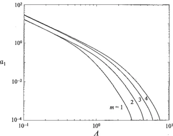
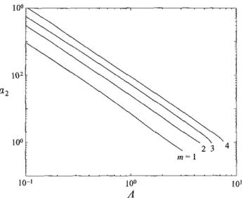
0:4 = — oc¡ for odd modes, and a¡~ = <x\ for even modes. (3.36) The constants OÍ\ and ccj are plotted in terms of A in figures 2 and 3; for the first

capillary mode, <xj" diverges at the capíllary instability limit, A = %, where our analysis breaks down, as will be remarked in §3.5.

The coefficients £í3, íf4 and fí5 in the amplitude equation (3.36) will depend on the

terms of orders sCl/2 and e2 in the expansions (3.1), which are considered now. When

taking into account (3.14), (3.21), (3.26)-(3.28) and (3.32), the solutions of (3.26), (3.5)—(3.13) for k = 1 and 2 are seen to be as given by

«i = AUiéQt + c.c, wi = A W ^1 + c e ,

qx - AQ,éQt + c e , /i = AF^' + c e , (3.37)

u2 = A2U22e2iat + c e + «20, w2 - A2W22e2iQí + ce. + w20, (3.38)

qt = A2Q22t2iQt + c e + \A\2Q20, f2 = A2F22emt + c.c. + \A\2F20> (3.39)

where the non-oscillatory (in the short time scale) components of the velocity field, i/20 and w20> will be considered in §5, while (UuWuQuFi), {U22,W22,Q22,F22) and

(620,^20) are as given by (A10)-(A19), in the Appendix. Notice that the problem (3.5)—(3.13) for k = 1 is solvable precisely because Hi is as given in (3.32), and that the problem (3.5)—(3.13) has a soíution for k = 2 only if neither Q\ = 2Q ñor £2} = 0

102F

10-2,

i<H

FIGURE 2. The coefficient «i in the leading term of the damping rate for the first four modes.

Q2

RGURE 3. The coefficient ctf/Q2 in the forcing term of the amplitude equation (3.3a) for the first four modes. The sign of a j is indicated.

Now H3, i/4 and H5 are calculated upon substitution of (3.1) and (3.36) into

(3.316) (witñ/2,---,^f as given in (A2)-(A4), in the Appendix) and setting to zero the

coefficients of eC, s2Cí/2 and s3, to obtain (after some tedious algebraic manipulations)

H3 = -a2A, H4 = 0, H5 = ia3Á\Á\2, (3.40)

where the real constants a2 and a3 are given by

(a2~2~2a¡/Q) í F0(z)Q0(l,z)áz = (1 + i ) f QQÁr,A)Qlr{r,A)rár/{2üY2

J-A JO

+ / [ 2 e0( l , z )2- f i2f o ( 2 )2- ( l + i)a1F1(z)2o(l,2)]dz-4fíU)FÍ(yí), (3.41)

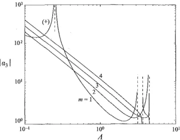
FIGURE 4. The coefficient «2 in the first correction to the damping rate for the first four modes. 2(a3/G) í F0(z)Qo(lí Z)dz- f [(2 - 3Í22)F0F22 - F^ + (2 - Í22)F0F20 - í j F ^

- 2 ^0( í , z ) ^2 2( l , z ) - ( F2 2 + F20)Q0(l,2)]Fodz+ í (F22 - F2o)W0(l,z)2d2

+

'-A .h

(11F0 + \W¿)F^ + 4(F0 + F»)FÜF0 - (6 + Í22)F03

-F0^o(l,z)2]F0dz/2. (3.42)

In order to obtain (3.41)—(3.42) we have taken into account that it/o, iWo» 60 and F0 are real (see (3.5), (A9o) and (A.9b)); we have also used (3.32), (3.35) and the

equations

/ f (UoUi + WoWfr&dz** f [-adl-mQoiUVQ-FiQoiUzHáz, (3.43)

J-A JO J-A

[iV¡r + Vi + W¿ + W¿)r + U¡/r] áráz

=^4F,0(A)F,¿{A)+ f [£32F2 + 2FÍQ0{l,z)]dz, (3.44)

J-A

which are obtained after some manipulations of the problems giving {Uo, WO,QO,FQ)

¡máiVitWuQuFi).

A plot of the constants a2 and a3 in terms of A is given in figures 4 and 5 for the

first four inviscid modes. Notice that for m = 1,0C3 diverges at the capillary instability limit, A — n, and at A ~ 0.249 (where 2Ü is also an inviscid frequency); there are other divergences of «3 that either correspond to higher-order modes or to valúes of A that are greater than %.

3.5. Validity limits of our weakly nonlinear description

1 U F " •• 1. . ) i

10-' 10° 101

A

FIGURE 5. The coefficient a3 in the cubic term of the amplítude equation (3.3a) for the first four modes. a3 Ís always negative except for the part of the plot corresponding to the first mode that is

indicated with the sign (+).

(a) If either 2Q or fí/2 is also an inviscid eigenfrequency, or more generally, if there are two additional inviscid eigenfrequencies, QÍ and Q2, such that Q+Q\ ±Ü2 = 0, then

our analysis is not valid because it ignores the coupled effect of other inviscid modes that may also be excited. In this case, two or three coupled amplitude equations, with quadratic nonlinearities, must be considered that exhibit chaotic behaviour (Mancebo, Nicolás & Vega 1996). Similarly, if there are three additional inviscid eigenfrequencies, Qu Q2 and ¡Q3 such that Q + Ü\ + Q% ± Q3 = 0, then we should

consider two, three or four coupled amplitude equations, with cubic nonlinearities. Higher-order parametric resonances do not affect the validity of our analysis in the time scales we are considering.

(b) Our analysis also breaks down if there is a second inviscid eigenfrequency such that either |í^i - Q\ ~ 5 oí \Qi - Q\ < $ (with 3 = a.\Cl¡2 + a2C, see §4)

because then the inviscid mode associated with Q\ is also excited and its coupled effect cannot be ignored. This may in fact occur for high-order inviscid modes as we see now. The frequency of the mth inviscid mode, Üm, is such that Q^/imn/lA)3, -» 1

as m —> co (see (A6)); then Üm+\ — Qm ~ m^2 as m —> oo. On the other hand, it

may be seen that ai ~ Ql/2 and a2 ~ Í34/3 as Ü —»• oo. Then our analysis is valid

only if we are exciting the mth inviscid eigenmode with m3C2 <C 1 (for £3„1+i — Qm

to be large as compared with <S), i.e. with QmC < 1. Otherwise we must take into

account the coupled effect of infinitely many inviscid eigenmodes (with frequencies •••, Qm-2, Í2m_i, Qm+u Qm+2> "X that add up to a pair of counterpropagating,

modulated capillary wavetrains that interact nonlinearly and exhibit dispersión and refíection at the disks. Any further discussion on these wavetrains is of course beyond the scope of this paper.

(c) The characteristic size of the Stokes boundary layers is of the order of {C¡Q)X¡1

(see §3.2) and must be small compared to A (the size of the liquid bridge) for the analysis above to make sense. That condition fails (in the interval 0 < A < %) in two limits: as A ~ C2 or A <C C2 (because Q ~ A"2^2 as A —* 0 for a fixed inviscid

first inviscid eigenmode, whose associated eigenfrequency is of the order of (n —A)1/2

as A —»• n. We shall not pursue these limits any further because they are somewhat distant from the main object of the paper.

4. The amplitude equation

The amplitude equation (3.3b), with Ht, * • •, H¿ as given by (3.32) and (3.40) may

be written as

E5^ =, -f i [(l+i)alCl/2+a2C] A+icc383A\A{2+ifiocÍ f^+e1£ü+t - (-l)'7_ei ( ü-T]+ HOT,

(4-1) where we are using (3.36), m is the order of the mode being excited and

HOT = O {eC^1 + e5 + fi{s2 + CL/2)) ,

as found after a somewhat carefuJ analysís. The real constants <xu a2, c¿3 and a j are

as gíven by (3.33)-(3.34) and (3.41)-(3.42) and plotted in figures 2-5 for the first four modes. Notice that «i and cc2 are aJways positive, while «3 and a j may be either

positive or negative, depending on the mode being excited and the slenderness. Notice that the forcing term vanishes if co+ = a>_ (i.e. the forcing frequencies of the

disks are equal) and either (i) m is even and /f+ = /L (i.e. an even mode is excited

and the disks are vibrated in phase, with the same amplitude) or (ii) m is odd and j8+ — — /í_ (i.e. an odd mode is excited and the disks are vibrated in antiphase, with

the same amplitude). In both cases, higher-order terms should be considered in (4.1) to calcúlate the forcing term, and the complex amplitude evolves on a still larger time scale.

We now define the small parameters S, s and \i as

5 - aiCV!1+a2C, £ - (¿/|«3|)l/2, /* = ^> í4-2)

and re-scale the complex amplitude A as

A = i{jS+B/ÍjM)eÍG)+T if a3 > 0, A = -i(j5+B/¡j5+¡)eiíü^ if a3 < 0, (4.3)

to rewríte (4.1) as

dB/dx = - ( 1 +ia>t)B + iB\B{2 + Af(l + iVei(ü3T), (4.4)

where we are ignoring HOT, we are assuming that /í+ ^ 0 and

a>i = (t»+ + a1Cl/2/5)a3/\ct3\, ™i = (aj_-fl)+)a3/|«3l, M - a+|0+|, (4.5)

JV = ( - l)m+l^/p+ if cc3 > 0, N = ( - l)m + 1/L/0+ if a3 < 0. (4.6)

Notice that the real parameters M, a>\ and to2 and the complex parameter N may be

seíected itidependently by appropriately choosing the forcing frequencies, amplitudes and phases. Two cases must be distinguished.

4.1. Periodic osciüations: /L. = 0 or co+ =

co_-If either N = 0 (i.e. only one disk is vibrated) or oj2 — 0 (i.e. the vibrating frequencies

of the disks are equal) then (4.4) may be written as

dB/dt = - ( 1 + ÍCO0B +iB|S|2 + AÍ!, (4.7)

where

We now briefly justify a well-known property of (4.7), namely that its solutions converge to a steady state as x —• co. To see that we first multiply (4.7) by B and add to the resulting equation its complex conjúgate to obtain

d|B|2/dT - ~2\B\2 + MiB + MXB. (4.9)

This equation readily iraplies that

\B\ ^ \M\\ as T -» co,

i.e. the orbits of (4.7) are bounded. Then, according to Poincaré-Bendixon theorem (Perko 1991), every orbit of (4.7) aproaches either a steady state or a closed curve of the phase plañe as T —• oo; but the latter cannot occur, according to Bendixon criterium (Perko 1991) (because if (4.7) is rewritten as a second-order system of real equations, áx/át = f{x), then the divergence of the vector field f is div / = —2 < 0 for all vectors x).

The steady states of (4.7) are readily calculated by means of the following pair of real equations:

|£|[cos<p + (¡B|2-<üi)sin<?>] - |Mi|, (4.10)

(|fí|2-coi) eos <p - sin q> = 0, (4.11)

where <p is the phase of B/M\. The variable q> may be eliminated from (4.10)-(4.11) to obtain the following cubic equation in \B\2:

|B|2tl + (|B|2-©1)2l = |Af1l2. (4.12)

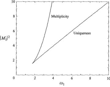
The bifurcation diagram of that equation is plotted in figure 6. The equation possesses exactly three solutions in the multiplicity región, two solutions in the boundary of that región, vvhich is given by

|M1|2-2[co1(co2+9) + (co2-3)3 / 2]/27, with coi > yfi, (4.13)

and a unique solution in the remaining part of the (tí)t, \M\ |2)-plane. Also, it is readily

seen that when (4.12) has three solutions, 0 < |B(i < \B\2 < ]B|3, the steady state of

(4.7) corresponding to |B|2 is unstable, and the other two are asymptotically stable;

when only one solution exists, it corresponds to an asymptotically stable steady state of (4.7). If |Mi|2 (resp. tuj) is kept fixed, the solutions of (4.12) may be plotted in

terms of a>í (resp. |M¡j2) by means of a curve that is monotonic if (MJ2 < (4/3)3/2

(resp. o), < yj3) or S-shaped if |Mi|2 > (4/3)3/2 (resp. a>i > ^3), as shown in figures 7

and 8. For a fixed valué of ¡M(¡2, the máximum valué of \B\ equals \Mi\ and it is

attained at a\ — \Mi\2.

Finally, notice that the asymptotically stable steady states of (4.7) correspond to orbitally asymptotically stable periodic solutions, of period 2n¡{Q + Sa>+), of

(2.1)-(2.9) (with the velocity and pressure fields in the bulk and the shape of the free boundary being given by (3.1)).

4.2. Quasi-periodic oscillations: /í_ =£ 0 and m+ =f= o)~

Now N ^ 0 and co2 =£ 0 in (4.4) (see (4.5) and (4.6)) and this equation must be

10

8

6

4

2

0 2 4 6 8 10

FIGURE 6. Bifurcaüon diagram of (4.12).

2.0

1.6

1.2

0.8

0.4

0

- 8 - 4 0 4 8

FIGURE 7. Solutions of (4.12) in íerms of a)i for \M\\ íixed. Asymptotically stable and unstable steady states are indicated with solid and dashed lines respectively.

if \o)2\ < 1, coi = 3.3, M = 2 and N = 1/2 then that parí of the S-shaped

curve in figure 8 between Mv = 1 and Mi = 3 is slowly followed (in the time

scale x ~ l/|co2¡) in the manner indicated by the arrows. These osciUations may

be approximately described by means of matched asymptotic expansions (Grasman 1987). For the sake of brevity we do not pursue this (fairly standard) matter any further.

In order to obtain the attractors (as T —• oo) of (4.4) for generic valúes of the parameters we have used a numerical continuation technique (Keller 1987) that allows us to follow continuous branches of periodic solutions when three of the four parameters (cou «>2» M and N) are kept íixed and the fourth one is varied. For the sake of brevity we only give a rough description of one of the bifurcaüon diagrams obtained in this way.

2.5

2.0

i.5

\B\

1.0

0.5

0 2 4 6 8 10

\M¿2

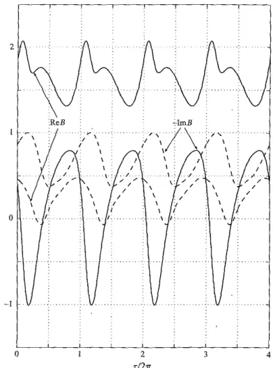
FIGURE 8. Solutions of (4.12) in terms of \M\\2 for ÍÜI fixed. The arrows indícate the path followed by relaxation oscülations of (4.4) when jro2| <.l,cot= 3.3, M = 2 and N ~ 1/2.

That bifurcation diagram corresponds to tO] = 3.3, M — 2 and a>2 — —1, for varying real valúes of the parameter N (that raay be assumed to be real without loss of generality because its phase may be annihilated by means of an appropriate translation in the time variable). If N = 0 then (4.4) lias two exponentially stable steady states, B = 0.217 - 0.622Í and B = 1.811 + 0.585Í (and a third unstable steady state). If 0 < N < Ni ~ 0.217 then (4.4) possesses two asymptotically stable periodic solutions of period 2n; those corresponding to N = 0.21 are plotted in figure 9. At N — JVj that stable periodic solution exhibiting larger valúes of

\B\ loses stability through a supercritical period-doubling bifurcation, and a new branch of asymptotically stable 47r-periodic solutions appears; the asymptotically stable solutions at N = 0.22 are plotted in figure 10. At N = N2 ^ 0.224 the

47c-periodic solution exhibits a new supercritical period-doubling bifurcation and if N2 < N < N3 — 0.227 then (4.4) possesses two asymptotically stable periodic

solutions, of periods 2n and Hn; those corresponding to N = 0.225 are plotted in figure 11. At N = iV3 the bifurcated 87ü-periodic solution disappears through

a reversed supeicritical period-doubling bifurcation and the branch of 47i-periodic solutions becomes asymptotically stable again. In the interval N3 < N < N4 ~ 0.271 several bifurcations of various types take place, which are not considered for the sake of brevity. If N > N4 then (4.4) has only one asymptotically periodic solution,

of period 2n, The bifurcation diagram is invariant under the symmetry N —> — N (because (4.4) is also invariant under the transformation N —* ~N, z —» T + 71/012)-Notice that all periodic solutions of (4.4) considered here generically correspond to quasi-periodic oscülations in the liquid bridge.

5. Streaming flow in the bulk

The terms of order e2 in the expansions (3.1) of the velocity field in the bulk, u2 and

w2, were not completely calculated in §3 (see (3.38)) for their slowly varying parís,

FIGURE 9. Asymptotically stable 2jr-periodic orbits of (4.4) (plotted with solid and dashed lines),

for ioi = 3.3, M = 2, co2 = - 1 and N = 0.21.

whích are independent of the short (capilíary) time variable, and may be seen as the leading-order terms of the components of the time-averaged (in the short time scale) velocity field in the bulk; they are given by

«20r + ^1120 -f" W20z = 0,

|*3|«2>i + W2o(tÍ20Z— W2Qr) = ~«70f + V(«2Qrr + «20zz + r~1«20r ~ r2« 2 o ) »

1CÍ3|W20T +W20(W20r-U20z) = "«70* + 7Í^20rr +^20zz +Í""1 W20.),

W20 - i-B|2gf (r), W 2 0 - O at z - ± ¿ ,

W20 = w ^ = ^702 = 0 at r = 0,

W2Ü = |Sl2g2(z), w20i- = !-B12g3(z) at r = 1,

(5.1) (5.2) (5.3) (5.4) (5.5) (5.6)

where z, a3 and 5 are as given in (3.4), (3.42) and (4.2)~(4.3), q^ is that parí of the

term of order e4 in the expansión (3.1) of the stagnation pressure field in the bulle, #7»

FIGURE 10. Asymptotically stable periodic orbits of (4.4), of periods 2% and 4n (plotted with

dashed and solid lines respectively), for co\ — 3.3, M — 2, (x¡i = —1 and JV = 0.22.

and the functions gf, gi and g3 are given by

y = \a2\C/(alC^2 + a2C),

gfOO = - [3(1 -iWoüor + c.c. + 4r-1\U0\2]^±A/2Q, (5.7)

g2(z) - [F^WQ -F0Üor + c.c.]r=], (5.8)

g3(z) - i [3(2íjv + 2f? - Q2F0)F¿ + ( ^ ' + F¡>) K] fü ~ [^brr^o]^ + ce. (5.9)

Notice that, according to the usual valúes of ctít a2 and tx3 (see figures 2, 4 and 5),

the constant y may be considered as an 0(1) quantity for realistically small valúes of C, e.g. C £ 10"5 (even though y -> 0 as C -y 0). Equations (5.1)-(5.3) and (5.5) are

obtained upon substitution of (3.1) into (2.1)—(2.3) and (2.5), setting to zero that part of the terms of order s2 in the resulting equations that is independent of the short

T '—f !—~—~~T~ ~—i "—T '——r

FIGURE 11. As in figure 10 but now the periods are 2TC and 8n, and N = 0.225.

In order to obtain (5.2) and (5.3) we have taken into account that

Í£2~' \A\2Ü0Wo [r~l(W20r - U20z) - (W20(- - t*2Qz)í-] + c.c. = 0,

~{iQ-i\A\2U0W0lw20r-u20z)z+ C.C.] £ 0 ,

as readily seen when taking into account that, according to (3.5), (A7)~(A9ÍZ) and (A9b), UQ and WQ are purely imaginary. If the left-hand sides of these two equations were non-zero (as happens to be the case for non-resonant oscíllations, see Nicolás et al, 1996a) then they should be added to the left-hand sides of (5.2) and (5.3) respectively; these two additional terms are obtained as the short-time averages of (AW$Q>Qt + c.c.)(usz — vv5r) and (AUQG1^ + c.c.)(w5z — wsr) respectively, where

us =iÜ'lAW0&Ql(u2üZ-W2Qr)+ cc. + q5r + NRT and w5 = ií2_1¿4£/0eiQí(u20r-W2<k) +

cc. + q¡z + NRT are the components of the velocity field at order e3 (and NRT

stands for non-resonant terms, as in the Appendix).

Since Uo is either symmetric or antisymetric in the z-variable, FQ is real and UQ and WQ are purely imaginary (see (3.5), (A9a) and (A9f?)), we have

FTGURE 12. The funcíion gj1" = g, associated with the first natural mode, giving the forcing radial

velocity in the boundary condition (5.4), for severa! valúes of the slenderness.

In adition, the net tangential radial flux at the disks is seen to satisfy

\B\2 f rg±{r)dr =-~\B\2 / |£/0(r,/l)|2dr/2fl < 0. (5.11)

Jo Jo

A plot of the forcing term gf = gj~ associated with the first natural mode is given in figure 12 for several valúes of the slenderness.

The model (5.1)—(5.6) provides the (Eulerian) short-time-averaged velocity that, for kinematical reasons, needs not coincide with the drift (or mass-transport) velocity, that is, the (Lagrangian mean) velocity associated with the short-time-averaged trajectories of material elements; notice that the drift velocity must be used for comparison with experiments. But, since our osciílating field is standing (that is, its phase is independent of position) in first approximation, both velocities do coincide (Batchelor 1967) and (5.1)—(5.6) also provides the drift velocity field.

Now, if either (i) only one disk is vibrated or (ii) both disks are vibrated with the same frequency then, as seen in §4.1, |B| evolves to a steady state as % —>> oo. If the initial transient is ignored, then \B\2 may be considered as a constant in (5.4)

(that may be calculated, as a steady state of (4.7), in terms of the non-dimensional frequency detuning tüi and forcing amplitude ¡Mj|; recall that (4.7) may exhibit up to three steady states). If, in addition, \B\2 is not too large (to avoid flow instabilities)

then the solution of (5.1)—(5.6) evolves to a steady state as T —> oo. If the eigenmode being excited and the slenderness are kept fixed, then the forcing function gf remains constant and that steady state depends only on the parameter

k = \B\2/y, (5.12)

as readily seen when dividing u2o and w2o by y, and g70 by y2 in (5.1)—(5.6).

0.3

0.2

0.1

W20(1,Z)

I5I2 -0.1

- 0 . 2

- 0 . 3 < - — ^ _ - — _ u _ — . ~ _ ^ _ _ — _ i

-1-0 -0,5 0 0.5 1.0 z

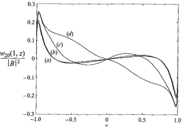
FIGURE 13. Axial velocity ai the interface for the steady streamirtg due to the first mode at A ~ 1. {a) { ) k = % (—-—) íc = 20 (mdistinguishable), (b) k = 200, (c) k = ÍO0O, (d) fc = 2000.

The resulting axial velocity at the interface, w2o{{,z)/\B\2, and the streamlines are

plotted in figures 13 and 14. Several remarks concerning these results are in order. (a) Both the axial velocity at the interface and the streamlines in figures 13 and 14 are quite representative of other numerical results obtained for higher-order natural modes and for other valúes of the slenderness.

(b) The flow pattern is always symmetric on the plañe z ~ 0; thus only one half of the liquid bridge is plotted in figure 14, even though numerical calculations were made in the whole domain, 0 < r < 1, — 1 < z < 1, to ensure that no symmetry breakíng appears in the range of k considered.

(c) The quantity w2o/|S|2 = w2o/yk and the streamlines are almost equal for fe = 2

and 20 (see figures 13 and 14a). This means that «20/7 and qio/y2 depend linearly

on k if 0 < k ^ 20 and thus satisfy the (Stokes) linear problem resulting from neglecting convective terms. This was to be expected because, in two-dimensional incompressible flows in finite containers resulting from steady forcing at the boundary, the zero-Reynolds-number limit frequently appíies up to fairly large valúes of the Reynolds number.

(á) For k = 2, 20 and 200 the flow pattern exhibits two small toroidal eddies near the corners, r — 1, z = +1, that push the liquid away from the disks along the interface, and two larger counter-rotating (toroidal) eddies in the bulk (that push the liquid towards the disks along the interface). Again, this was to be expected; the small eddies are due to the fact that the forcing radial velocity at the disks is positive in a small región near the corners (see figure 12), and the large eddies are due to the fact that the net forcing radial flux is negative (see (5.11)). These flow patterns are in rough qualitative agreement with the experimental observations by Mollot et al. (1993, figure 12).

1.0 o

FIGURE 14. Streamlines for the five cases ín figure 13. Flow patterns are always symmetríc and only one half of the capillary bridge is plotted.

5.1. The combined effect of vibration and thermocapillary stress

Let us now consider the combined effect of the steady forcing terms due to vibration and the thermocapillary stress in non-isothermal conditions. We shall consider a distinguished limit when (a) the temperature is independent of the fast (capillary) time í in first approximation, and (b) thermocapillary stress produces a velocity field in the bulk that is of the same order as that associated with the streaming flow considered above (that is, of the order of s2). As a consequence (c) the oscillating

considered. But the derivation below could be more easily followed íf the dependence on the slow time variable is ignored. For the sake of brevity, the derivation below is not given in full. See Nicolás et al. (1996a) for a more detailed derivation of a related asymptotic model that exhibits the same features as that below and applies to the non-resonant case.

In order to model thermocapillary effects, the tangential stress balance at the interface (2.7) must be replaced by

{Wr±uz){l-fl) + 2{ur~Wz)fz = -{CRe){\+fl)lí\ez+fzer) at r = / , (5.13)

where Re is the effective (or thermocapillary) Reynolds number, defined as Re — ff7(AT)R/pv2 (with AT a typical temperature increment in the íiquid bridge, crT =

da/dT the thermal gradient of surface tensión, p the density, v the kinematic viscosity and R the radius of the disks, as defined in §2), and 0 is a non-dimensional temperature (Q = (T - T0)/(Ti - T0), where T0 is the temperature of the disks and T± is a

characterístic temperature in the Íiquid bridge), that satísfies the energy conservation equation

o

+ ue

+ wO

= {c/p){e

+ r

e

+ e

) (5.14)

and boundary conditions

0 = 0 at z = ±A, (),. - / A = (1 + jl)1'1 g(z) at r - / . (5.15)

Here P — pvcp/ko (cp is specific heat, &0 is thermal conductivity) is the Prandtl number

and g = g(z) is the non-dimensional normal heat flux through the interface, that is assumed to be given and symmetric, i.e. g(—-z) = g(z). As is usual in the literature, we are assuming all properties of the Íiquid to be independent of temperature except for surface tensión, which depends linearly on temperature in first approximation. That dependence is taken into account only in the tangential stress balance boundary condition at the interface (where that dependence appears at leading order, in the right-hand side of (5.13), and not as a correction to somethíng larger). The thermal boundary conditions (5.15) are the simplest ones giving symmetric thermocapillary flows, which are of interest in materials processing as indicated in §1.

We shall consider the distinguished limit

Re ~ P - 1, (5.16) but our asymptotic model below may be seen to apply to larger valúes of the Reynolds

number, namely whenever

Re < C~l.

Notíce that if thís condition holds then the velocity and pressure fields associated with the thermocapillary stress are such that u, w and q are small (even though the thermocapillary Reynolds number may be large) and the thermocapillary flow can be considered as a perturbation of the quiescent state when analysing the oscillatory flow (with the non-dimensionalízation based on the capillary characterístic time we are using in this paper); thus the analysis in §3 remains valíd (except for the boundary condition (5.20) below).

Now, the temperature in the bulk is expanded as

6 = OQ(r>z,T) + s[A01éat+ c e ] + HOT (5.17)

(5.2)-(5.3)). Notice that (even though we are interested only in the leading-order term OQ) we aíso need to consider a first correction of order e, that oscülates in the fast (capillary) time scale, t ~ 1. If (3.1) and (5.17) are inserted into (5.14) and the coefficient of e is set to zero, then ©\ is seen to be as given by

0i = UiUodor + WQBQz)¡Q. (5.18)

Notice that temperature oscillations in the bulk are driven only by the oscillating velocity field through convective eífects; heat conduction comes into play to calcúlate temperature oscillation only in the oscillatory boundary layers (Le. in regions (a) and (b), see figure 1). Similarly if the non-oscillatory part (i.e. that part that is independent of the fast time variable t) of the coefficient of e2 is set to zero, and the defmition

(4.2) of g is used, then we obtain

0OT + W2ü£W + w20e0z = (y/P)(90rr + r-l90r + <W, (5.19)

where y is as defined in (5.7) (recall that y may be considered as a 0(1) quantity in practice); thus, in the limit (5.16) y/P may be considered as an 0(1) quantity and, according to (5.19), the time scale x ~ 1 coincides with the thermal time scale. In order to obtain (5.19), we have taken into account that Á(UQ0h. + WQ0ÍZ) + c.c. = O,

as readily seen when using (5.18) and the fact that UQ and WQ are purely imaginary (see (3.4), (A9a) and (A9b)) and 90 is real. If this additional term were not zero

(as happens when the oscillations are non-resonant, see Nicolás et al, 1996a) then it should be added to the left-hand side of (5.19); notice that this term is obtained as the short-time average of (^[/oeií3í + c.c.)(É>1(.eií3t + c.c.) + (J4Woeií3' + c.c.){0Isei£3t + c.c.).

Finally, when using the new boundary conditions (5.13) and (5.15) in the analysis of the Stokes and the interface boundary layers (see §§3.2 and 3.3), and applying the appropriate matching conditions with the solution in the bulk, then we obtain the new boundary conditions

w2o = 0, w ^ = -yRedÜ2 at r = 1, (5.20)

0Q - 0 at z - ±A, 0o, = g(z) at r = 1, (5.21)

where we have used the defmition of e (in (4.2)) and (5.10).

Now, the model posed by (4.7), (5.1)-(5.5.) and (5.19)-(5.21), with cou Mu y and gf

as given by (4.5), (4.8) and (5.7), gives the combined effect of the slowly varying forcing terms due to vibration and thermocapillary stress. For the numerical applications below we assume the non-dimensional heat flux through the boundary to be given by a Gaussian, Le.

g(z) = exp(-az2/2), (5.22)

as usually done in the literature to model the heat flux through the interface when considering applications to the float zone technique.

As above, we shall consider only steady flow patterns. Then we may consider B as a parameter (that may be calculated as a steady state of (4.7)). Also, the steady states depend only on the parameters k (see (5.12)) P and Re, and on the forcing functions gf (see (5.7) and figure 12) and g (see (5.22)).

400

>"20(l.g)

- 4 0 0

-1.0 -0.5 0 0.5 1.0

Z

1.2

0.8

0.4

-1.0 -0.5 0 0.5 1.0

z

FIGURE 15. Axial velocity and temperature at the interface for the steady fiow in the buik at A = 1

due to vibration of the first mode with k — 2000 and thermocapillary effects with P — 0.02: (ÍI) Re = 100, (&) Re = 500 and (c) Re = 2000.

(except near the corners, but this is a localized eíFect) if k < 200. That prediction is confirmed by some numericaí calcuíations that are not presented for the sake of brevity.

For larger valúes of k (e.g. k = 2000), counterbalancing is (a priori) possible because the streaming fiow due to vibration and the purely thermocapillary fiow exhibit essentially opposite structures near the interface. In order to elíucidate whether effective counterbalancing is feasible, the problem (5.1)—(5.5), (5.19)-(5.22) has been numerically integrated for A — 1, P = 0.02, k ~ 2000, a = 2 and three valúes of the thermocapillary Reynolds number, Re = 100, 500 and 2000. The axial velocity and the temperature at the interface and the streamlines are plotted in figures 15 and 16. Two remarks concerning these results are in order:

(a) As in figures 13 and 14, these ñow patterns are representative of counterbalanc-ing results for other (non-limitcounterbalanc-ing) valúes of the parameters. Also, the fiow pattern is always symmetric in figúrelo, where only one half of the liquid bridge has been plotted.

thermo-1.0 o

FIGURE 16. Streamlines for the three cases in figure 15. Flow patterns are always symmetric and only one half of the capillary bridge is plotted.

capülary stress untü the eddies near the córner become quite localized (see figure 16c). Nevertheless the máximum valué of the velocity at the interface remains unaffected (see figure 15). This is due to the fact that the boundary condition at the disks, (5.4), is independent of thermocapiUary effects, and illustrates the main diificulty that makes these streaming flows inconvenient to counterbalance thermocapiUary convection in the whole liquid bridge. Nameiy, the price for any possible counterbalancmg effect in the bulk is the introduction of large velocities near the corners.

Therefore nearly inviscid, almost-resonant, low-frequency vibration is not effective to counterbalance thermocapiUary flows in liquid bridges. In order to get effective counterbalancing, the forcing tangential stress at the interface coming from vibration, W20r(l>z) — \B\2g3{z) (see (5.6)) plays an essential role; it vanishes here (see (5.10))

Water Mercury 1 03x C

ítfxd

l t f x e itfXjlf 10-1 x k

MI

ÍO4 x a (cm)

103 x tc (s)

ÍO"2 x Ú (Hz)

102 x Afl (cm)

10 x vs (cm s_1)

10 x v¡ (cm s"1)

TABLE 1. Vibrating parameters and steady streaming results for A = 1, R = 1 mm, if the first eigenmode is excited by vibration of one disk.

(1996a). Also, if the vibrating frequency is large enough to excite a large number of capillary eigenmodes (i.e. Q ~ C~v > 1) then these modes add up to a pair

of progressive counterpropagating wavetrains along the interface, which have been analysed by Nicolás et al. (1996b), who have shown that the associated streaming flow is quite effective in counterbalancing symmetric and non-symmetric thermocapillary flows. In both cases the steady tangential stress at the boundary is non-zero and may be selected to have the right shape (by appropriately choosing the vibrating parameters) to counterbalance thermocapillary stress.

6. An application in laboratory dimensional parameters

For illustration, let us consider two capillary bridges, of water and mercury (p = 1 and 13.63 gm cm~3, a = 72 and 484dynescm-1 and v = 0.89 x 10~2 and 0.113 x

10~2 cm2 s_1 respectively, at 25°C). If the radius of the disks is R = 1 mm (a typical

* valué for mülimetric liquid bridges) then the small parameter C — {pv2/aR)^2 is as

given in table 1. If, in addition, the slenderness is A ~ 1 and the first eigenmode is excited then Q ~ 3.3 (obtained from the first equation of (A6), in the Appendix), the coefficients in the amplitude equations are ai ~ 0.09, a2 ^ 7, a3 — —2.5 and

a\/Q2 cu 0.25 (see figures 2-5)), and the small parameters <5, e and ft are as given

in table 1 (and obtained from (4.2)). Now, for our analysis to be valid, e\A\ <C 1. Then we take coi = \Mi\2 = 16 and 64 respectively in equation (4.12), whose upper

solution (there is also a lower, stable solution at these valúes of co¡ and |Mi|) is \B\2 = )Mi|2 = 16 and 64 respectively. If only the upper disk is vibrated then

M = |Afi| and \A\ = \B\ (see (4.3) and (4.8)), and /í+ and h are readily calculated

from (4.5), (5.7) and (5.12), to be as given in table 1. Now, the dimensional vibrating amplitude, a = 2¡x\fi+\R (see (2.11)), the characteristic time tc — {pR3/<r)1/2 and the

dimensional vibrating frequency, Q — (Q + 5(ú+)/27ttc (with co+ as given by (4.5)), are

readily calculated. Similarly, since the máximum of the eigenfunction F0 {given by

(A7) in the Appendix) equals 0.235, the máximum deflection of the interface in one oscillation is ¿1/J, — 2£\A\\Fo\maxR, Finally, with these small valúes of the parameter

h (59 and 280) the streamlmes of the associated streaming flow are qualitatively similar to those in figure 14{a, b), and the velocities in the small and large eddies in dimensional terms are vs = £2\B\2w\QR/tc and v¡ = E2\B\2w2QR/tc respectively, with

w¿ c¿ 0.2 and w|0 ~ 0.03 (see figure 13).

Notice that we are obtaining fairly large streaming velocities with very small oscillatory deflection of the interface. Our results suggest that only the first two patterns in figure 14 are obtained in millimetric liquid bridges if we maintain the

condition of small oscillatory defíection of the interface (that requires e\A\ to be appropriately small), excite the first mode and take A ~ \ (the physical properties of other liquids or liquid metáis are not different enough to those considered above to allow significantly smaller valúes of e). This might explain why only the first two patterns in figure 14 were obtained by MoUot et al. (1993) for low-viscosity liquids. The situation is different if we excite high-order modes (Nicolás et al. 1996a, b), significantly lower the slenderness A or increase the radius of the disks. In space platforms, R may be as large as 5cm; if, for example, mercury is used and \A\ = 17, then C — 8.5 x 10"5, s = 0.024 and k may be as large as 2000; then the last two

patterns in figure 14 can be also obtained.

7. Concluding remarks

We have considered the weakly nonlinear axisymmetric, nearly inviscid oscillations in a liquid bridge resulting from almost-resonant, axial vibrations of the disks. A cubic amplitude equation has been derived for the complex amplitude of the oscillating pressure and velocity fields and of the oscillating shape of the interface. That equation is a balance between inertia, damping, detuning from resonance, nonlinearity and forcing, and includes a second approximation in the damping term (in order to ensure a quantitatively good approximation for realistically large valúes of the capillary Reynolds number) and a first approximation of the remaining effects.

The coefficients of the amplitude equation have been calculated in terms of the slenderness and the inviscid mode being excited, and the large-time behaviour of the solutions have been discussed. In particular, we predict the liquid bridge to exhibit periodic oscillations when either only one disk is vibrated or both disks are vibrated with the same frequency. Typical response diagrams in terms of the forcing frequency exhibit hysteresis when the forcing amplitude is not too small; this hysteresis has not been detected experimentally (perhaps because most experiments in the literature seem to have been designed to confirm linear theories that do not predict that effect), but some recent experiments with pendant drops (De Paoli et al. 1995) showed the effect. If both disks are vibrated with different (but appropriately cióse) frequencies then we predict that generically the capillary bridge exhibits quasi-periodic oscillations with two frequencies, one of them aímost equal to the forcing frequencies and the other one of the order of the difference between them. Typical response diagrams now exhibit multiplicity and period doubüngs that, again, have not been detected experimentally.

The Stokes boundary layers near the disks produce a steady (or slowly varying) forcing radial velocity that has been also calculated. The resulting slowly varying flow have been considered in §5, where some experimental observations by Mollot et al. (1993) have been explained and other non-observed flow patterns have been predicted. Also, the combined effect of the steady forcing terms due to vibration and thermocapillary stress have been analysed in §5.1, to conclude that this streaming flow is not effective in counterbalancing thermocapillary convection. But our results suggested how to get the required effect (see Nicolás et al. 1996a, b).

Finally, let us recall that our analysis requires several limitations that were discused in §3.5.

Numerícal calculations in Sections 4.2 and 5 were performed by Mr. Marcos Vera and Dr. Damián Rivas respectiveiy. We are also indebted to Dr. Rivas for helpful discussions, and to the three anonimous referees for several criticisms and suggestions on an earlier versión of the paper that led to a significant improvement in the presentation. This research was supported by DGICYT and by the EEC Program on Human Capital and Mobility, under Grants PB-93-0046 and CHRX-CT-93-0413.

Appendix.

In this Appendix we give several groups of algebraic expressions that were omitted in §3 to facilítate the reading of this section. The first group deals with the integral expressions appearing in the solvability conditions (3.31b), which may be written as

h = S f f (Uouz + W0wx)rdrdz

J-A JO

- 8 / [fJQo + (f - D / r O o r ~ ( / - l ) ( ü " 0 « r + W0WT)]^áz

J-A

+ 2ecÍH{eiat f í UQ(r,A)[ÜQ(r^) - Uo(r,¿)]rdrd£ + c.c. j + HOT, (Al)

13 = - CzAéat í f [{Ul + üi + Wl + Wl)r + Vl¡r] drdz + NRT + HOT, (A 2)

J-A Jo

U= ( {s{fW0(l,z) + {f ~\)WoAUz))(AWZ{0,z)éQt+c.c.) +iQ(l-f/2)F0ft

J-A

+ (f-l)[ft{UUhz) + Uo(Uz))-fQQl.(l,z) + FQ-hF'¿}

- /

( / - l )

( ^ + ^ ) } /

d

- i í 3 ^ | ( / " l )

( l - f i

/ ) + ( / - l ) /

+ |/

(l+AJ

+ ^ V W ( 0 , z ) e

+ c . c . ) ^

- i [ft+&\AWZ{G,z)éQt + z.c)2]Xáz + ~ J ( / - l )3C ^ ( l ,2) d z

+ Í [ C / o r r ( / - l )2/ 2 - W o , /^( / - l ) ]r = 1( / - l + / „ ) d z - c /, f[zWo{U)áz

J-A J-A

+ C / [ /r+e( ^ ( 0 , z ) el Q Í+ c . c . ) ] U0(l,z)áz + HOT, (A3)

J5± = (ifí/^±ei í Q f _ U ± T ) + c.c.') í rQ0(r,±A)ár

±Cl/2s í Uo(r,A)\AUod^O)éat + c.c. + Cl/2üH(r,0)^eü2í(r,0))rár+íiOT, (A4) Jo *- • 1

where u and w (the veíocity components in the bulk) and / are as given in (3.1), U0> W0, «i, u2 and WQ are as given in (3.16H3.18) and (3.25), NRT stands for

being an integer), and

HOT = OÍJÍ + BC + E2C1 / 2 + £3). (A 5)

Also, in order to obtain (A1)-(A3) we have used the solution in the Stokes boundary layer near z = — A (not given in §3.2), the facts that U^r.A) = W0r(r,A) = 0, that

the ñinctions £/¿ and UQWQZ are even in the z-variable and that W¿(Qtz) = Wa(ítz)

is purely imagmary and F0 is real (see (3.5), (A9a) and (A9b); also, in order to obtain

(A 3) we have used the equation

if - l)/Qo(l, 2)dz = -ifí / [/•(/ - 1) + 2 /2 + (2/ - l)/zz]F0dz + ofou),

which is obtained upon substitution of (2.9), (2.11), (3.7) and (3.8), and integration by parts.

The linear eigenvalue problem (3.5)—(3.8), may be solved in a semi-analytical form, as first shown by Sanz (1985). The eigenfrequencies are the real Solutions of one of the following equations:

A tan A = ~S~] anrn or A cot A-\- J ^ anr„ — 0, (A 6) ji odd fi even

where

a0 = 1, a„ = 2Q2/(Q2qu - sa) if n ^ 1, (A 7)

q» = HLl rn = q»/(l2n - í), s» =/«(/J - l)/i(/B), /„ = nn(!A if n > 0, (A8)

and J0 and ii are the first two modified Bessel functions. If the first equation of (A 6)

holds (odd modes), Qo and F0 are given (up to a common constant factor) by

Qo = ^2 aMLr)cos[ln(z + A)], FQ = Asinz/cosA + ^ <Vncos[í„(z + A)], n odd « odd

(A 9a) while if the second equation of (A 6) holds (even modes), then

Qo = 5 3 aMlnr)oos[ln{z +A)]> F0 = ^cosz/sin.4 + ^ a ^ c o s ^ í z +yl)]. TI even n even

(A 96) £/0 and WQ are readíly calculated by means of the second and third equations of (3.5).

The functions Q\ and F\ appearing in (3.37)—(3.39) are as given by

& = - ( 1 - i)[bQo + dQQ/dA] + J2 bnloikr)cos[ln(z + A)]¡{2Q)V\ (A 10)

n odd

fi - - ( 1 - i) [6F0 + 8Fo/dA + 2A{dQ/dA - a1(2í2)I/2sin2/(í2 eos A)]

+ 5^6BrflcosPI,(z + ^)]/(2fi)1^ (A 11)

ÍI odd

if £3 is a solution of the first equation of (A 6), or

fíi = - ( 1 -i)[6fío + dQo/dA] + £ V o í W c o s ^ z + A)]/(2Q)^\ (A 12)

n even

Fy = - ( 1 - i)[M?0 + 5^/5/1 + 2A{dQ/dA - ax{2Q)^2) cosz/(£3 sin^í)]

if Q satisfies the second equation of (A 6); Ui and W\ are

Ui = [ieir + íl-iJaiUol/fi, Wi = [iQi2 + ( l - i ) « i W b ] / a

Here the constant b„ is given by

6n = 2Q{dQ/dA - al{2Q)í/2)qllan/{Q2ql1 - sn) for n = 0 , 1 , . . . ,

(A 14)

and the constants a)}, /„, íj¡„ r„ and s„ are as given in (A7)-(A8). The results in the

paper (i.e. the coefficients íf3, H4 and H5 of the amplitude equation (3.3b)) do not

depend on thé constant b. The remaining functions appearing in (3.37)-(3.39) are given by

Q21 = 2Q2cQ + 4£32 ¿ C2kJ0(2/kr) cos[2/fc(z + A)], (A 15) fe=í

Í ^ Í K Í Z W Í U ) - ^ ) ^

¡t=l

C/22 = Í622r/2Í2, ^2 2 = Í022,/2O,

020 = i>3 - goA

íao = -»4 cosz - £>3 - 5 3 g a ( l - 4 © -1 cos[2/t(z + ¿)],

{A 17) (A 18) (A 19) where

/

A t»

F0(z)2dz/4^ + ^ [ saea + 2(1 - 4 © ^ f í2 Í 2 f c] / (4Q2q2k - Sat) (1 - 4l¡)

Z>2 - vi cot y( - 1 + 8Í22 J 3 ra/(4fi2 Í 2 f c - s2fc), /(=o

D* =

Dd =

t a n A 5 2 ( l - 4 ikV g 2 f c + / |Fo(z)|2dz/2

^ E (

-

í ) "

* » + / l

o(z)!

dz/2

(yl — tan A),

(A eos A — sin/í),

and for n > 0, the constants í„, r„, q„ and s„ are as given in (A 8), while c„, d„, e„ and g„ are as given by

cn = [2DJD2 + (1 - ¿„2)4/2 + eH] /(4fl2a, - s„),

dn = - Í / K ( z ) Í T o ( l , z ) - Jio ( z ) ü ' or( l , z ) ] c O S [ /J I( z + ^ ) ] d z / ( ^ l í 3 ) ,

e „ = / [ ( 2 - 3 Q2) F o ( z )2+ W o a z ^ - F i í z ñ c o s P ^ z + ^ d z / l y l ,

g„= í [ ( f í2^ 2 ) | f0( z ) f2- | ^0( l , z ) ¡2+ | ^ ( z ) |2] c o s [ /( ((Z+ ^ ) ] d z / A

J-A

Notice that as 2Ü approaches a solution of the second equation of (A 6), D2 —> 0 and