A Fuzzy approach based on dynamic programming and metaheuristics for selecting safeguards for risk management for information systems

A Fuzzy Approach based on Dynamic Programming and Metaheuristics

for Selecting Safeguards for Risk Management for Information Systems

E. Vicente, A. Mateos and A. Jimenez-Mart´ın

Decision Analysis and Statistics Group, Departamento de Inteligencia Artificial, Universidad Politecnica de Madrid, Campus de Montegancedo s/n, Boadilla del Monte, 28660 Madrid, Spain

Abstract: In this paper we focus on the selection of safeguards in a fuzzy risk analysis and management methodology for information systems (IS). Assets are connected by dependency relationships, and a failure of one asset may affect other assets. After computing impact and risk indicators associated with previously identified threats, we identify and apply safeguards to reduce risks in the IS by minimizing the transmission probabilities of failures throughout the asset network. However, as safeguards have associated costs, the aim is to select the safeguards that minimize costs while keeping the risk within acceptable levels. To do this, we propose a dynamic programming-based method that incorporates simulated annealing to tackle optimizations problems.

1 INTRODUCTION

There are several risk analysis and management

methodologies for information systems (IS) that con­

form to International Organization for Standardiza­

tion (ISO) standars, specifically the ISO 27000 fam­

ily of standars. Some examples of these method­

ologies are MAGERIT, by the Spanish Ministry of

Public Administrations (Lo´pez Crespo et al., 2006);

CRAMM (CCTA, 2003), by the Central Computing

and Telecommunications Agency (UK); or NIST SP

800-30 (Stoneburner and Gougen, 2002), by the Na­

tional Institute of Standard and Technology (USA).

These methodologies do not, however, consider

uncertain valuations, but use precise values on differ­

ent, usually percentage, scales. Boolean values are

sometimes even used to indicate whether or not assets

are dependent on each other regardless of the degree

of such dependency. In no case is vague or impre­

cise information about the input parameters allowed.

In our opinion, this is an important drawback of these

methodologies.

In (Vicente et al 2013a) we proposed an exten­

sion of the MAGERIT methodology based on clas­

sical fuzzy computational models. This methodology

includes the following milestones:

1. Identification and Valuation of Assets

An asset is anything that is of value to the or­

ganization and therefore requires protection. A

few data, information or business process assets

often account for the total value of an organiza­

tion’s assets. These assets are called terminal as­

sets. Other assets (support assets such as hard­

ware, software, personnel, facilities, ...) are valu­

able insofar as they are beneficial to the terminal

assets, and they inherit the terminal asset value,

according to the resulting benefit. Thus, support

assets have no intrinsic value; they take their value

from terminal assets.

The identified assets of the organization are then

valued. Some assets may have a monetary value

(how much money the organization would lose if

this asset stopped working), whereas others re­

quire a qualitative assessment (if an asset stops

working the losses would be very high, low,

medium...).

As mentioned above, the support assets inherit

their values from terminal assets depending on

how they influence each other. So, we have to de­

termine the dependency relationships of the termi­

nal assets with respect to support assets, and also

dependency relationships between support assets.

2. Threat Identification

cases, threats can cause different impacts

depend-ing on what assets are affected. A detailed list of

threats is available in Annex C of ISO IEC 27005.

MAGERIT suggests two threat assessment

mea-sures: degradation, the damage that the threat can

cause to the asset, and frequency, how often the

threat materializes.

3. Identification and Valuation of impact and Risk

Indicators

It is then necessary to qualitatively identify the

consequences and establish impact and risk

indi-cators for the valued assets and threats. The

im-pact of a threat on an asset is the product of the

asset value multiplied by the respective

degrada-tion. Risk is the product of the impact of the threat

multiplied by the respective frequency.

4. Selection of Safeguards

Safeguards are measures for addressing threats.

They can be procedures, personnel policies,

tech-nical solutions or physical security measures at

the facilities. These safeguards can be

preven-tive, if they reduce the frequency of threats; or

palliative, if they reduce the degradation of assets

caused by threats (Lo´pez-Crespo et al., 2006).

As described below, experts use a linguistic term

scale (see Figure 1 and Table 1) to represent asset

values, their dependencies and the frequency and

as-set degradation associated with possible threats. Risk

analysis computations are then based on the

trape-zoidal fuzzy numbers associated with linguistic terms.

However, direct assignment based on a rigid

lin-guistic term scale is not always advisable since the

expert has no say in the number of linguistic terms

that the scale is to include and about the appearance of

their associate trapezoidal fuzzy numbers. In that case

we propose the use of the betting and lottery-based

method for fuzzy probability elicitation described in

(Vicente et al 2013c). Betting and lottery-based

meth-ods commonly used to assign probabilities can also

be used to assign fuzzy probabilities (Savage, 1954;

Finetti, 1964). In this section we briefly describe

these methods and show how a fuzzy number

rep-resenting the probability judgment can be extracted

from experts.

Betting Method. For two selected monetary values

x > y, the expert is given the option between either of

the two following gambles:

• b 1 : If event A happens, then you win x$.

Other-wise, you lose y$.

• b2: If event A does not happen, then you win y$.

Otherwise, you lose x$.

If the expert has no preference for either bet, the

respective expected utilities of both bets are equal,

and it follows that p(A) = x/(x + y). If the expert chooses one of the two gambles, then the expected utility of the selected gamble should be higher than for the rejected gamble. Then, the analyst has to up-date monetary values and offer the expert two new gambles. Thus, an interactive process is enacted un-til two alternative gambles are reached to which the expert is indifferent.

Lottery-based methods. For a given probability and monetary values x$ and y$, the expert is given the choice between the following lotteries:

• l1: If event A happens, then you win x$. Other-wise, you losey$.

• l2: You win x$ with probability p, or y$ with probability 1 —p.

If the expert has no preference for either of the lot-teries, then the respective expected utilities are equal, and it follows that p(A) = p. Otherwise, the expert must readjust the value p, keeping the same mone-tary values. This again generates an interactive pro-cess, enacted until a couple of lotteries are reached to which the expert is indifferent.

The betting and lottery-based methods assume that the expert is able to provide a specific value for the probability of an event. However, a more realis-tic scenario is where experts have an imprecise and vague idea of that value. Consequently, experts will have an interval rather than a precise value in mind at the point when they are indifferent to either bet or lot-tery, that is, for the lottery-based method there will be an interval [a, c] such that if p = [a, c], then the expert has no preference for either lottery l1 or l2. Similarly, the betting method can result in an interval of indif-ference [b,d\.

Current protocols for probability elicitation like the above recommend the use of several methods to test the consistency of the expert and the existence of bias. In this regard, the development of betting and lottery-based methods meets this recommenda-tion and establishes the following:

• If [a, c] n [b, d] = 0 , then the expert’s probabilistic judgment was inconsistent.

• If any of the intervals is contained in the other [a,c] C [b,d] (or [b,d] C [a,c]), then we as-sume that the trapezoidal fuzzy number (b, a, c, d) (or (a,b,d,c)) designates the expert probabilistic judgment.

• If [a, c] n [b, d] y^ 0 , is uncountable, and none of the intervals is contained in the other, then, as-suming that a < b < c < d, (a,b,c,d) designates the expert probabilistic judgment.

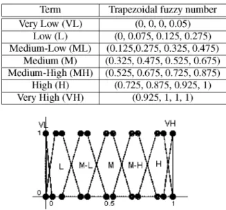
Table 1: Linguistic term scale.

Term

Very Low (VL)

Low (L)

Medium-Low (ML)

Medium (M)

Medium-High (MH)

High (H)

Very High (VH)

Trapezoidal fuzzy number

(0, 0, 0, 0.05)

(0, 0.075, 0.125, 0.275)

(0.125,0.275, 0.325, 0.475)

(0.325, 0.475, 0.525, 0.675)

(0.525, 0.675, 0.725, 0.875)

(0.725, 0.875, 0.925, 1)

(0.925, 1, 1, 1)

Figure 1: Linguistic term scale.

A = (a,b,c,d) with 0 < a < b < c < d < 1 and with a trapezoidal function in the vertices (a,0),(b,1),(c,1),(d,0) (Chen, 1996; Chen and Chen, 2003; Chen and Chen, 2009; Vicente et al., 2013b). Note that R is a subset of TF[0,1] if we consider the injection (Vicente et al 2013a) (|): R ^-> TF [0,1]; a « <\>(a) = (a, a, a, a) = a.

Consequently, the following operators proposed in (Xu et al 2010) accounting for trapezoidal fuzzy num-bers will be used to make computations:

Given A1 = (a1,b1,c1,d1), A 2 = (fl2,^2,C2,<i2) € TF[0,1], then:

• A1 © A2 = (a1 + «2 — a1a2,b1 + £>2 — b1b2,c1 +

C2 — c1C2,d1 -\-d2—d1d2) a n d

• A1 (g>A2 = ( f l1f l 2 j ^ 1 ^ 2 j C1C2,d1d.2).

© and eg) are two internal composition laws in TF[0,1] that verify the commutative and associative properties and both have a neutral element.

The assets of an IS are elements of value to the organization and therefore require protection (servers, files, personnel, facilities, hardware, software,...).

As cited before, these assets are interrelated (Lopez Crespo et al, 2006), forming an acyclic graph, where just a few data, information items or business process assets often account for the total value of an organization’s assets. These assets are called termi-nal assets. Other assets (support assets, such as hard-ware, softhard-ware, personnel, facilities,...) are valuable insofar as they are beneficial to the terminal assets. In other words, the support assets inherit their values from terminal assets depending on how they influence

each other, i.e., depending on the probability of that any failure in an asset being transferred to the termi-nal assets.

In general, we say asset Aj directly depends on asset A,-, denoted by A; —> Aj, if a failure in asset A; causes a failure in the asset Aj with any given prob-ability. This probability is usually referred to as the degree of direct dependency of Aj with respect to A,-. Note that in this fuzzy adaptation the degrees of di-rect dependency between assets will be represented by linguistic terms, which have associated trapezoidal fuzzy numbers. We denote these degrees of direct de-pendency by d(Ai,Aj).

These dependencies form a directed acyclic graph (to terminal assets), so that there may be intermediate assets between any asset A; and a terminal asset Ak which can propagate a fault generated in A,- through to the terminal A*. Our aim then is to compute the trans-mission probability between A; and A*. This proba-bility is called degree of indirect dependency between A; and A*, which is denoted by D(Ai,A]c) and can be computed as follows (Vicente et al 2013a).

We denote by P={P1,..., Ps} the set of paths in the network connecting A; with A*. These paths are a se-quence of arcs connecting a sese-quence of vertices, such that the start vertex and the last vertex are A; and A*, respectively. Then,

A) If all assets, excluding A,- and A*, in the paths in P are influenced by only one asset, then

LJ ( A i A h )

where D (A ,•, A k | Pj)

© D(AhAk\Pj) (1)

" ( A j j A j 1 ®d{Ah,A2) (g) ...®d(Ajn,Ak) and

J : v ' 71 J ->•

-+A

^A

).

B) Otherwise, we assume that the first r paths in P are formed by assets (excluding A,- and A*) influ-enced by only one asset, and the remaining s — r paths include at least one asset simultaneously in-fluenced by two or more assets. Then, for the r first paths, we proceed as in A), and we denote by S the set including the s — r remaining paths. We proceed with S as follows:

(i) Consider the set of non-terminal assets in S in-fluenced by two or more assets, denoted by 7, and the subset of I including assets uninflu-enced by any other asset in I, denoted by NI. (ii) We consider an asset Ar in NI. Then, we

(iii) Remove repeated paths f r o m S and keep only

one instance.

(iv) B u i l d / and NI again f r o m S.

(v) I f NI is not empty, go to ( i i ) . Otherwise, the algorithm finishes.

L e t us denote the resulting set o f paths b y S= {P[, •••iP'm\ w i t h m < s — r. Then, the degree o f dependency o f A^ regarding A; is

D(Ai,Ak) = © D(Ai,Ak\Pj) © D(Ai,Ak\Pi). (2)

7=1 l=1

Once we have computed the degree o f indirect dependency between all assets regarding the termi-nal assets, we can compute the accumulated values for non-terminal assets v~i. These values usually have three components (ISO/IEC serie 27000):

1. Availability. H o w much damage w o u l d i t cause i f the asset is not available or cannot be used? This is a typical services inspection.

2. Confidentiality. H o w much damage w o u l d i t cause i f the asset is disclosed to someone i t should not be? This is a typical data inspection.

3. Integrity H o w much damage w o u l d i t cause i f the asset is damaged or corrupt? This a typical data inspection. Data can be manipulated, be w h o l l y or partially false, or even missing.

Therefore,

7 ( \ D \ A { Afc) Cg) V£

k=1 il)

(3)

where / denotes the /th component.

Once assets have been valueted, the next step i n the risk analysis methodology is to identify possible threats and compute the corresponding impact and risk indicators for the IS.

Threats are characterized b y h o w often the threat materializes (frequency) f and b y the degradation D = (d1,d.2,d3) that the threat can cause to the three

asset components. Note again that the frequency and degradation levels w i l l be selected b y the expert f r o m the linguistic term scale and, consequently, a trape-zoidal fuzzy number w i l l be associated w i t h each o f them.

Then, the impact o f a threat on an asset Aj is

// — a^j (So v\

(i) *• (i

and the risk to the asset is

R, (0 /;,„ Cg) / .

(4)

(5)

The results of these operations will be fuzzy

num-bers belonging to TF[0,1], which, generally, do not

match up with the fuzzy numbers associated with the

linguistic terms of the scale. Thus, a similarity

func-tion must be used to identify the most similar

trape-zoidal fuzzy number in the linguistic term scale to the

fuzzy number output from computations.

Different similarity functions have been proposed

by several authors (Chen and Chen 2003, Chen and

Chen 2009, Gomathi and Sivaraman 2012, Xu et al

2010, Zhu and Xu 2012). In (Vicente et al 2013b) a

new similarity function was proposed on the basis of

the geometric distance between both fuzzy numbers,

the distance between their centroids and/or the ratio

between the common area and the joint area under the

membership functions.

Following the risk analysis and management

methodologies for IS, Section 2 deals with the

selec-tion of safeguards that can be enforced to reduce the

transmission probability of a failure throughout the

IS. The aim is to minimize costs while keeping the

risk at acceptable levels. To do this, we propose a

mixed technique based on dynamic programming and

metaheuristics, specifically, simulated annealing.

2 SELECTION OF PREVENTIVE

SAFEGUARDS

F r o m equations (3), (4) and (5) and the algorithm for computing degrees o f indirect dependency, we can de-rive the risk for the IS i n each component / given a

threat w i t h frequency / and degradation D = < di >

i n the support asset A; as

^ n ^ ^ ^

'(i) = iLDD{AiAk)eg)VK„ ®f®di, k=1

V]c(l) being the value (constant) assigned to the

termi-nal asset Ak i n the component /.

Safeguards are measures for addressing threats. They can be procedures, such as incident manage-ment and documanage-mentation; personnel policies, such as training and awareness o f employees operating on the IS; technical solutions, such as identification and authentication mechanisms based on biometrics; or physical security measures o f the facilities, such as temperature control systems.

In this section we propose a method for reducing the degrees of dependency from all support assets to terminal assets minimizing the costs for the company. As mentioned above, the probability of transmis-sion of failure D(Ai,Ak) is the result of fuzzy opera-tions with the probabilities of transmission of failure through intermediate assets linking the attacked sup-port asset with other asset.

In each of these intermediate assets, safeguards can be enforced to reduce the probability of transmis-sion of a failure. The effect induced for a safeguard in the probability of transmission of failures between two assets Au and Av can also be defined as a lin-guistic term, which is represented by a fuzzy number e"'v G TF[0,1], so that if the degree of direct depen-dency between the assets Au and Av is d(Au,Av), then, when we implement a safeguard with effect e"v, the degree of direct dependency is reduced to

d(A^A v )®(1e^v),

where 0 denotes the usual subtraction op-eration between trapezoidal fuzzy num-bers, i.e., (a1,0.2,0.3,0.4) © {b1,b2,b3,b4) = (fl1 — &4,fl2 - ^ 3 , ^ 3 — ^2,^4 — b1).

Note that 0 is not an internal composition law in TF[0,1], however,

• A,B G TF[0,1] => A(gi (1 © 5 ) G TF[0,1], • A 0 (1 © 5 ) < A with the partial order of the

trape-zoidal fuzzy numbers (i.e., A <B •$$• a1 <b1,02 < b2, «3 < b3, «4 < b4 ) and

• A 0 ( 1 0 B) decreases with B.

We consider the set of safeguards that hinder the direct transmission of failure between Au and Av, Su,v. Each safeguard Sup,v G Su'v has a monetary cost cp'v

over d(Au,Av), which is reduced to

d(Au,Av) 0 (1 Qep' ) .

The problem of keeping an acceptable level (low or very low) for the failure transmission probabilities among support and terminal assets with minimal costs can be represented as follows:

mm LLCp xp u,v p

S.t.

D{A~Ak) <UikVi,k ' xup'v G {0, 1 } V K , V , / ?

where i and k in the first set of constraints refer to non-terminal and terminal assets, respectively, [/& is a residual value accepted by the experts, xup'v are the de-cision variables (xp = 1 means that safeguard Sp is selected), and D(A{,Ak) is reassessed replacing values

d(Au,Av) by the affected values regarding the selected safeguards:

<f(Au,Av)0 0(1©2^'V) p

and an effect ep

where Au and/lv are two consecutive assets connected by an arc in some path between A; and A*.

Note that the fact that the usual order in TF [0,1] is a partial order constitutes a very restrictive constraint in our optimization problem, so we w i l l use the con-cept of similarity function to relax this constraint.

If we define a threshold a G [0,1] and a similar-ity function S, the constraint D(A,-, A*) < [/;* Vi, k can be replaced by S(D(Ai,Ajc),Unc) > oc. Thus, the re-strictiveness of the constraint increases proportionally to the threshold value and the feasible solution set w i l l be composed of solutions that verify these soft-ened/relaxed constraints.

Remember that indirect dependencies are recur-sively computed following the algorithm described in Section 1. Thus, the degree of dependency of the support assets further away from the terminals can be computed from the degree of dependency of the closest assets. Therefore, the problem can be solved in stages, and the principle of optimality in dynamic programming is verified: Given an optimal sequence of decisions, every subsequence is, in turn, optimal. Then we proceed as follows:

• Let L0 be the set of terminal assets.

• Consider L1 including support assets whose chil-dren belong to L0 only (L1 is not empty because the graph is acyclic). Identify safeguards that min-imize costs keeping the degrees of dependency over their children at an acceptable level.

• Consider L2 including support assets whose chil-dren belong to L0 U L1 only. Identify safeguards that minimize costs keeping the degrees of depen-dency over L0 under an acceptable level. Note that the degrees of indirect dependency from the chil-dren of L2 to terminal assets have already been computed in the previous stage, so we just need to identify the direct degree of dependency over assets in L0 U L1.

Simulated annealing (Kirkpartick et al 1983, Cerny 1985) is applied in each step of the algorithm to de-rive the optimal selection of safeguards. It is a trajec-torial metaheuristic which is named for and inspired by annealing in metallurgy.

An initial feasible solution is randomly generated. In each iteration a new solution y is randomly gen-erated from the neighborhood of the current solution, y G N(XJ). If the new solution is better than the cur-rent one, then the algorithm moves to that solution (x,-+1 = y), otherwise the movement to the worst solu-tion is performed with certain probability.

Note that accepting worse solutions allows for a more extensive search for the optimal solution and avoids trapping in local optima in early iterations.

The probability of accepting a worse movement is a function of both the temperature factor and the change in the cost function.

The initial value of temperature (T) is high, which leads to a diversified search, since practically all movements are allowed. As the temperature de-creases, the probability of accepting a worse move-ment falls. If the temperature is zero, then only better movements will be accepted, which makes simulated annealing work like hill climbing.

The pseudocode of simulated annealing for a min-imization problem is as follows:

• Generate an initial feasible solution X0. D o X* = X0, f* = f(x0), i = 0.

Select the initial temperature t0 = T (?,- tempera-ture in the step i)

• Repeat until stopping criterion is satisfied: - Randomly generate y G N(xi)

* If f{y) — f(xi) < 0, then • xi+1 = y

• If f(x*) > f{y), then x* =y,f* = f(y) * Else

• p ~ £/(0,1)

• If p < e-( / M-/ W ) A ' , thenx;+1 =y • Elsex;+1 =xi

– i = i-\-1

- Update temperature

3 AN ILLUSTRATIVE EXAMPLE

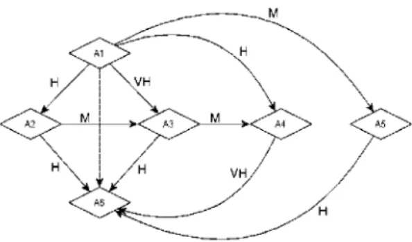
Let us consider the IS shown in Figure 2 with the

di-rect degrees of dependency assessed by the experts

considering the linguistic terms of Table 1, which has

only one terminal asset, A

.

Figure 2: Direct dependencies in the IS.

The set of paths in the analysis of the influence of A1 over A6 is P = {

• P1 : (A1 —> A2 —> A6), • P2 : (A1 —> A2 —> A3 —> A6), • P3 : (A1 —> A2 —> A3 —> A4 —> A6), • P4 : (A1 —?>A3 —> A6),

• P5 : (A1 —> A3 —> A4 —> A6), • P6 : (A1 —> A4 —> A6), • P7 : (A1 —> A5 —> A6)}.

Asset A3 is influenced by A1 and A2, and A4 is influenced by A1 and A3. Therefore, we proceed as in B) of the algorithm described in Section 2, with r = 2 and S= {P2,P3,P4,P5,P6}, as follows:

(i) I = {A3,A4} andNI = {A3}.

(ii) Select A3, then simplify paths P2, P3, A and P5 to - P2 : (A1 —> A3 —> A6),

- P3 : (A1 —> A3 —> A4 —> A6), - P4 : (A1 —> A3 —> A6) and - P5 : (A1 —> A3 —> A4 —> A6),

respectively, with <f(A1,A3) = D(A1,A3) = (d(A1,A2)®d(A2,A3)) ®d(A1A3). (iii) S= {P2,P3,P6 } since P'2 = P4 and P3 = P5. (iv) / = {A4} and NI = {A4}.

(v) Go to (ii).

(ii) Select A4, then simplify paths P'3 and P6 to - P3 : (A1 —> A4 —> A6), and

- P6 : (A1 —> A4 —> A6),

respectively, with d(A1,A4) = D(A1,A4) = (d(A1A3)®d(A3,A4)) ®d(A1,A4). (iii) S= {P^P3} sinceP^ = P6.

(iv) I = 0 y NI = 0.

Finally, S= {P^P3 and the degree of dependency of A6 regarding A1 is D(A1,A6) = D(A1,A6\P1) ©

DiMMP7) ®jHA^\P^)j^D(A^\Pf) =

(d(A1,A2) <g>d(A2,A6)) © (d(A1,A5) <g>d(A5,A6)) © (rf(A1,A3)(8)rf(A3,A6))e(rf(A1,A4)(8)rf(A4,A6))

The degree of dependency of A6 regarding A1 is D(A1,A6) = (0.980,0.999,0.999,1) if we consider the linguistic terms of Table 1 show in Figure 3.

Let us consider a threat on asset A1 with frequency f = M and degradation d = (H,H,H), then the risk to asset A1 is R1(l) = (0.23,0.415,0.485,0.675), / = 1,2,3.

We consider the asset network and the fuzzy direct dependencies shown in Figure 2 corresponding to an IS. Besides, the set of available safeguards of failure transmission between support assets are shown in Ta-bles 2-5.

We also consider the fuzzy threshold U = (0,0,0.1,0.2) below which the degree of dependency between all assets and terminal assets will be accept-able, and let a = 0.95. In other words, the similar-ity of the degree of dependency after applying the se-lected safeguards for the given U must be at least 0.95.

The set of solutions in each stage is represented by binary matrices, in which each row represents the safeguards of S"v, which prevents the failure transmis-sion from asset u to v considered in that stage.

We use the similarity function proposed by (Chen 1996): Given two trapezoidal fuzzy numbers A = ( a 1 , f l 2 j f l 3 j f l 4 ) a n d B = (b1,b2,b3,b4),

Table 2: Safeguards for A1.

4

S(A,B) = 1

I CLi — bi |

4

Although other similarity functions have been pro-posed in the literature (Chen and Chen 2003, 2009, Sridevi and Nadarajan 2009, Xu et al 2010, Hejazi et al 2011, Gomathi and Sivaraman 2012, Zhu and Xu 2012, Vicente et al 2013b), we have decided to use the geometric distance between both fuzzy numbers due to its low computational cost.

Dynamic programming is then executed as fol-lows:

First, note that L0 = {A6}, since the only terminal asset in the IS in Figure 2 is A6.

• Stage 1: L1 = {A4,A5}. We adjust the degrees of dependency

D(A4,A6) d(A4,A6) 0

VH 0 0 ( 1 0 ep' Xp ) LP

d(A5,A6) 0

0 ( 1 Qep xp ) p

and D(A5,A6)

0 (1 © e,p Xp )

_p

Tag

r1,2

13 1

r1,2 ^2 1,2 S3 r1,2 J4 01,2 5 1,2 6 1,2 7 r1,2 ^8 r1,2 J9 14 s14 1,4 S3 1,4 4 01,4 5 1,4 6 14 1,4 8 1,4 J9 1l,4 1,4 11 1l,4 S 2 Tag r,2,3

1 31

r,2,3 ^ 2

2,3 S3

2 4

S 2 5'

c2,3 6 r,2,3 c2,3 8 r,2,3 J9 Effect L M M H M M L L V L M H V H M M M H V H M M M M H H L M Table Effect M L M L M M L M M M L Cost 100 300 550 430 125 240 100 324 570 209 267 342 789 234 356 276 200 467 342 127 207 Tag r1,3

13 1

r1,3

, 32 1,3 S3 r1,3 J4 1 ,3 5 1 ,3 6 e ,3 1 7 1 ,5 131 r1,5

, 32

1,5 S3 1.5 4 1 ,5 5 1 ,5 6 r1,5

, 37

1 ,5 8 r1,5 J9 Effect M H H L M L V L M H M M M L M M H H M H M M

3: Safeguards for A2.

Cost 356 87 267 320 156 320 256 300 200 Tag r,2,6

13 1

r,2,6

, 32

2,6 S3 02,6 4 02,6 5 c2,6 6 r,2,6

, 37

c2,6 8 r,2,6 J9 1 2,6 r,2,6 1 2,6 02,6

51 3

Effect M L M L M L M L M M L M L M L M L M L Cost 356 324 110 345 87 345 200 230 345 187 321 345 543 356 206 342 Cost 348 187 254 367 567 390 256 307 235 124 400 278 260

H 0 0(1 0£p' ^p' )

such that S(D(A 4 ,A 6 ),U) > 0.95 and s (D(A 5 ,A 6 ),U) > 0.95,2J being the effect induced for the safeguard

-5,6

1,..., 10, ep the effect induced for the 4,6

5,6

safeguard S5p,6, p = 1 4,6

1 5 4,6

Table 4: Safeguards for A3. Tag (,3,4 ^ 1 c3,4 ^ 2 3,4 S3 c-3,4 J4 c.3,4 ^ 5 c-3,4 ^ 6 c.3,4 ^ 7 c.3,4 ^ 8 c.3,4 •59 Effect M H M M M H L L M Cost 345 650 200 367 388 453 189 256 345 Tag c-3,6 ^ 1 c,3,6 ^ 2 3,6 S3 c,3,6 J4 c-3,6 ^ 5 (,3,6 ^ 6 c-3,6 ^ 7 Effect M M M M M M M H Cost 267 356 378 324 345 231 453

Table 5: Safeguards for A4 and A5. Tag

4 1' c.4,6 ^ 2 4,6 S3 c.4,6 J4 e4,6 ^ 5 c.4,6 6 c.4,6 J7 c4,6 8 c.4,6 J9

1 4 , 6 5o Effect M M ML M M M M M M MH Cost 260 245 170 256 367 289 278 345 240 435 Tag 5 1' 5,6 ^ 2 5,6 S3 5,6 J4 „5,6 ^ 5 5 ,6 6 c.5,6 J7 e5,6 8 c.5,6 J9 e5,6 10 c.5,6

^ 1 1

c.5,6

J1 2

c.5,6

J1 3

c.5,6

J1 4

c.5,6

51 5

effect M M L ML M MH MH M ML L M M M L MH Cost 200 210 120 234 267 367 366 254 145 206 306 345 280 178 377

respectively, and x5p,6 = 1 or x5p,6 = 0 depending on whether or not the safeguard S5p,6, p = 1,...,15, minimizing the cost.

As L1 contains two elements, two optimization problems must be solved in this stage, associated with A4 and A5, respectively.

Regarding asset A4, solutions are represented by the vector x4,6 = (x41,6,x42,6,...,x41 ,06), see Table 5, where x4p,6 = 1 if the safeguard S4p,6 is selected. The respective optimization problem to be solved using simulated annealing is:

4,6 4,6 4,6 4,6

min

c x +

+ c x

S D(A 4 ,A 6 ),U > 0.95 Xp € { 0 , 1 } , p = 1,..., 10

(6) Cost o o o CM o o o

"i i i i r 200 400 600 800 Time

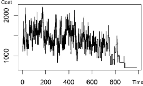
Figure 3: Objective function evolution in the optimum set-ting of D(A5,A6).

shown in the second row of Table 6, correspond-ing to vector x4'6 = (0,1,1,1,0,0,0,0,1,0). Regarding asset A5, solutions are now represented

5,6 5,6 5,6

by the vector x5,6 = (x51

5. The optimization problem to be solved is: x51 ,56), see Table

5,6 5,6

min c1 %1

5,6 5,6 • + c15x15 S.t.

S D(A 5 ,A 6 ),U > 0.95 Xp € {0,1},/? = 1,..., 15

(7)

The optimal solution and the associated costs are

The evolution of the objective function over time for the best solution found is shown in Figure 3. The optimal solution and the associated costs are shown in the first row of Table 6, corresponding to vector x5'6 = (1,0,0,0,0,0,1,0,1,0,0,0,0,0,0). The new degrees of dependency after the applica-tion of the selected safeguards and the respective similarity to the fixed threshold, U, are shown in the first two rows of Table 7.

The purpose of this paper is to describe how a mixture of dynamic programming techniques and metaheuristics can efficiently solve the problem and not to detail or compare the applied meta-heuristic (simulated annealing) with others. How-ever, we do think it is worthwhile to describe some parameters used in the implementation and to re-port a sensitivity analysis analyzing the effects caused by the changes to these parameters. - We randomly generate a sequence with binary

values and check if the similarity constraint is verified to derive the initial solution. The length of the binary sequence depends on the problem (15 when dealing with x5'6, 10 when dealing withx4'6...).

solution is not feasible (does not verify the sim-ilarity constraint), then it is discarded and an-other solution is generated in the neighborhood until a feasible solution is found.

The initial temperature assures acceptance probabilities of worse solutions close to 0.9 in the initial iterations of the algorithm. The ini-tial temperature is computed to obtain a high probability of acceptance ( > 0.9) of any neigh-bor of the initial solution, i.e., given the initial solution x0, the minimum value T is computed such that

e-(f(y)-fW)/T > 0.9, \/y e N(x0) and feasible,

Table 6: Optimal solutions and costs for each asset.

with:

f{y) — f(x0) > 0.

In other words,

T = max

yeN(x0) feasible

(f(y) — f(x0)) ln(0.9)

because if we have T > -(/(y)-/(*0))

_{Vy e}

ln(0.9)

JV(X0) and feasible, w i t h / f j ) — f(x0) > 0, then /«(0.9) < ~ u W - / W ; ; y-y g N(x0) and feasible, with f(y) — f(x0) > 0, and since e* is an increasing function, 0.9 < e T vy £ N(x0) and feasible, with f(y) — f(x0) > 0. The pseudocode, starting from x0 = (x0[1], ...,x0[«]), as follows:

* y = x0, T = 0, i = 1.

*• While i < n. Do y[i] = 1 —y[(\.

• If y is a feasible solution then, if ~i(0 9) > T, we have

T = (f(y) —/(x0)) /«(0.9) • y = x0, i = i+ 1.

The solution x0 has at most n feasible boring solutions. We have evaluated all neigh-boring solutions that are worse than the initial solution in those n steps.

In the unfortunate event that the initial solu-tion is the worst of its neighborhood, the initial value of the resulting T is null. Therefore we must start from another initial solution. This does not degrade the algorithm, because it can return to the neighborhood of the discarded so-lution at any time.

Thus the initial temperature that leads to the op-timal solution over A 5 (for optimization prob-lem (7)) is 3578.191.

Asset

^ 5

A4

A

A-2

A1

Solution

r5,6 r5,6 r5,6

4,6 4,6 4,6 4,6

S

, S

, S

,S

r r 3 , 6 r r 3 , 6 r r 3 , 6 r r 3 , 6

r*2,3 n2,6 n2,6 n2,6 r*3,6

(1,2 (1,3 (.1,4

Total cost

Cost

711

911

1275

1551

1236

5684

The temperature is maintained constant for L = 20 iterations and then it decreases after multi-plying by 0.95, so that, after h * L iterations, the temperature is th*L = 0-95h 0.

- The algorithm stops if / has not improved in the last 100 iterations.

Table 7 shows the best solutions reached after run-ning the algorithm with different values for a to minimize D(A5, A6). Note that if the constraint is more restrictive, allowing only minor differences with the threshold U, the set of safeguards for im-plementation will be larger. The same effect oc-curs when we use a more accurate (with a smaller support) threshold U. Therefore, experts must choose lower or higher levels of acceptable ac-curacy regarding the dependency between assets, i.e., the accepted risk considering this fact. • Stage 2: L2 = {A3}. The degrees of dependency

d{A3 A6) and d{A3 A4) are adjusted by minimiz-ing costs and incorporatminimiz-ing the soft constraint

© SD(A.3 ,A 6 ),U > 0.95, where

D(A3,A6) =

Lf(A

A

)g>

d(A3,A6)(g> g> (1Qep' Xp )

v>=1

g> (1ef/x

/) ) <g>D(A

,A

)

P

=1

Note that D(A4,A6) was

in Stage 1, D(A4,A6)

computed VH g> (1©«2 >

®{1Qt

)®{1Qt

)

(0.016,0.072,0.104,0.269). The optimization

problem to be solved in this stage is

3,6 3,6 mm C1 X1

3,4 3,4

c 1 1

3,6 3,6 .

. + C

X

+

3,4 3,4 • 1 Co -^Q

SD(A 3 ,A 6 ),U > 0.95 Xp'6G{0, 1},p= 1,...,7 Xq € {0,1} ,q= 1, ...,9

Table 7: D(A^,A(,) and associated costs for different a levels.

oc

0.8 0.9 0.95 0.98

D(A5,A6)

(0.05,0.23,0.27,0.46) (0.02,0.09,0.12,0.30) (0.01,0.07,0.11,0.28) (0.00,0.03,0.06, 0.20)

Similarity

0.81 0.93 0.95 0.98

Cost

554 653 711 1021

shown i n the t h i r d r o w o f Table 6, correspond-ing to vectors x3'6 = ( 1 , 0 , 0 , 1 , 0 , 1 , 1 ) and x3'4 = ( 0 , 0 , 0 , 0 , 0 , 0 , 0 , 0 , 0 ) . The new degree o f depen-dency after the application o f the selected safe-guards and the corresponding similarity to the fixed threshold, U, are shown i n the t h i r d r o w o f Table 7.

• Stage 3: L3 = {A2}. The degrees o f

depen-dency d(A2,A3) and d(A2,A(,) are adjusted m i n i

-m i z i n g costs and incorporating the soft constraint

s (D(A 2 ,A 6 ),U) > 0.95 , where

D(A2,A6) =

<f(A2,A3)©

d(A2,A6)®> i3 / T „ ~ 2 , 6 2,6 N

© [lQep xp ) © 2,3 2,3

© ( l e e ? Xp'3) ®D(A3,A6) P=\

Note that D(A3,A(,) was computed i n Stage 3,6

2, D(A3,A$) = [d(A3,A(,) © ( 1 0 e{ ) ® ( 1 0

3,6 3,6 3,6

£4' ) © ( 1 © e6' ) © ( 1 © e7' )] © [d(A3 A4)) ©

D(A4,A6)} = (0.008,0.059,0.096,0.301).

The optimal solution and the associated cost are

shown i n the fourth r o w o f Table 6,

correspond-ing to vectors x2'3 = ( 0 , 0 , 0 , 0 , 0 , 0 , 1 , 0 , 0 ) and

x2'6 = ( 1 , 0 , 0 , 0 , 1 , 0 , 1 , 0 , 0 , 1 , 0 , 0 , 0 ) . The new

degree o f dependency and similarity to U, are

shown i n the fourth r o w o f Table 8.

• Finally, L\ = {A\}. The degrees o f dependency

d(A\,A2), d(A\,A3), d(A\,A^) and d(Ai,A$) are

adjusted m i n i m i z i n g the cost and considering the

soft constraint S [D(Ai,A(,),u\ > 0.95, where

D\ A1 Afi,)

1,2 1,2

d(AhA2)(g>l ®(lQep' xp' )\®D(A2,A6)

d(A\ A3) © ( © (ieep'3xp'3) ) © £ ) ( A3, A6)

d(Ai,Ai)® I © (lQep' Xp ) I ©£>(A4,Ag)

rf(Ai,A5)© ( © ( T © 4 '54 '5) ) ©D(A5,A6)

N o t e that D(A2,A6), D(A3,A6), D(A4,A6) and

Table 8: New degrees of dependency after applying safe-guards.

Asset

A5 A4 A3 A2

A i

D(Aj,A6)

(0.015,0.077,0.114,0.280) (0.016,0.072,0.104,0.269) (0.008,0.059,0.096,0.301) (0.008,0.057,0.094,0.316) (0.005,0.045,0.082,0.327)

Similarity U

0.953 0.959 0.956 0.953 0.951

Figure 4 : Risk i n each component of A1 before and after implementation of optimal safeguards

D(A$,A(,) were computed i n previous stages, D(A2,A(,) = [d(A2,A(,) © ( ( 1 © g j ' ) ©

2,6 2,6 _2,6 1

(1 © £5' ) © ( 1 © ej ) © ( 1 © e^Q))] ©

\d(A2A3) © ((ioe-j ) ) © D(A3,A(,)] =

(0.008,0.057,0.094,0.316),

D(A3,A6) = (0.008,0.059,0.096,0.301),

D(An,A(,) = (0.016,0.072,0.104,0.269) and D(A$,A(,) = (0.01,0.07,0.11,0.28).

The optimal solution i n this stage is shown i n the last r o w o f Tables 6 and 7.

After implementing the best safeguards, the risk caused b y the previously considered threat over asset A\ i n each component is

tfi ₍₀ = (0.001,0.018,0.039,0.22), / = 1,2,3.

The risks associated with this threat before and af-ter implementation of safeguards are illustrated along with the risk threshold in Figure 4.

4 CONCLUSIONS

Although a metaheuristic could be used to solve this optimization problem, dynamic programming combined with simulated annealing was used because of the special structure of the constraint set. This leads to a more computationally efficient solution to the safeguard selection problem. Also the fuzzy environ-ment allows experts to provide imprecise and vague failure propagation probabilities.

Another way to reduce system risk is to act on the probability of threats to each asset materializing or re-ducing the degradation of assets caused by threat ma-terialization. This is a multiobjective problem (degra-dation has three components), which will be consid-ered in future research.

ACKNOWLEDGEMENTS

The paper was supported by Madrid Regional Gov-ernment project S-2009/ESP-1685 and Spanish Min-istry of Science and Innovation project MYTM2011-28983-C03-03.

REFERENCES

Cerny, V. (1985). Thermodynamical Approach to the Trav-eling Salesman Problem: An Efficient Simulation Al-gorithm, Journal of Optimization Theory and Appli-cations, 45, 41-51.

Chen, S.-M. (1996). New Methods for Subjective Mental Workload Assessment and Fuzzy Risk Analysis, Cy-bernetics Systems, 27, 449-472.

Chen, S.-J. and Chen, S.-M. (2003). Fuzzy Risk Analysis Based on Similarity Measures of Generalized Fuzzy Numbers. IEEE Transactions on Fuzzy Systems, 11, 45-56.

Chen, S.-J. and Chen, S.-M. (2009). Fuzzy Risk Analy-sis Based on the Ranking of Generalized Trapezoidal Fuzzy Numbers. Applied Intelligence, 26, 1-11. CCTA Risk Analysis and Management Method (CRAMM),

Version 5.0. London: Central Computing and Telecommunications Agency (CCTA), 2003. Finetti, B. (1964). Foresight: its Logical Laws, its

Sub-jective Sources. In: H.E. Kyburg and H.E. Smokler (eds.), Studies in Subjective Probability. New York: Wiley.

Gomathi, V.L. and Sivaraman, G. (2012). A Novel Simi-larity Measure between Generalized Fuzzy Numbers. International Journal of Computer Theory and Engi-neering, 4, 448-450.

ISO/IEC Serie 27000 International Organization for Stan-dardization.

Hejazi, S. R., Doostparast, A. and Hosseini, S.M. (2011). An Improved Fuzzy Risk Analysis based on a New Similarity Measures of Generalized Fuzzy Numbers. Expert Systems with Applications, 38, 9179-9185.

Kirkpatrick, S., Gelatt., C.D. and Vecchi, M. P. (1983). Optimization by Simulated Annealing. Science, 220 (4598), 671-680.

Lo´pez Crespo, F., Amutio-Go´mez, M.A., Candau, J. and Man˜as, J.A. (2006). Methodology for Information Sys-tems Risk. Analysis and Management (MAGERIT ver-sion 2). Book I, Book I I and Book III. Madrid: Minis-terio de Administraciones Pu´blicas.

Savage, L. J. (1954). The Foundations of Statistics. New York: Wiley.

Sridevi, B. and Nadarajan, R. (2009). Fuzzy Similarity Measure for Generalized Fuzzy Numbers. Interna-tional Journal of Open Problems in Computer Science and Mathematics, 2, 111-116.

Stoneburner, G. and Gougen, A. (2002). NIST 800-30 Risk Management. Guide for Information Technology Sys-tems. Gaithersburg: National Institute of Standard and Technology.

Vicente, E., Jime´nez, A. and Mateos, A. (2013a). A Fuzzy Approach to Risk Analysis in Information Systems. Proceedings of the 2nd International Conference on Operations Research and Enterprise Systems, 130-133.

Vicente, E., Mateos, A. and Jime´nez, A. (2013b). A New Similarity Function for Generalized Trapezoidal Fuzzy Numbers. Lecture Notes on Computer Science, 7894, 400-411.

Vicente, E., Jime´nez, A. and A. Mateos, A. (2013c). An in-teractive method of fuzzy probability elicitation in risk analysis, Intelligent Systems and Decision Making for Risk Analysis and Crisis Response, New York: CRC Press, 223-228.

Xu, Z., Shang, S., Qian, W. and Shu, W. (2010). A Method for Fuzzy Risk Analysis based on the New Similarity of Trapezoidal Fuzzy Numbers. Expert Systems with Applications, 37, 1920-1927.