Spatially-variant noise filtering in magnetic resonance imaging: A consensus-based approach

Spatially-variant noise filtering in magnetic resonance imaging: A

consensus-based approach

Luis González-Jaime , Gonzalo Vegas-Sánchez-Ferrero , Etienne E. Kerre

Santiago Aja-Fernández

A B S T R A C T

In order to accelerate the acquisition process in multiple-coil Magnetic Resonance scanners, parallel tech-niques were developed. These techtech-niques reduce the acquisition time via a sub-sampling of the k-space and a reconstruction process. From a signal and noise perspective, the use of a acceleration techniques modify the structure of the noise within the image. In the most common algorithms, like SENSE, the final magnitude image after the reconstruction is known to follow a Rician distribution for each pixel, just like single coil systems. However, the noise is spatially non-stationary, i.e. the variance of noise becomes x-dependent. This effect can also be found in magnitude images due to other processing inside the scanner. In this work we propose a method to adapt well-known noise filtering techniques initially designed to deal with stationary noise to the case of spatially variant Rician noise. The method copes with inaccurate estimates of variant noise patterns in the image, showing its robustness in realistic cases. The method employs a consensus strategy in conjunction with a set of aggregation functions and a penalty function. Multiple possible outputs are generated for each pixel assuming different unknown input parameters. The consensus approach merges them into a unique filtered image. As a filtering technique, we have selected the Linear Minimum Mean Square Error (LMMSE) estimator for Rician data, which has been used to test our methodology due to its simplicity and robustness. Results with synthetic and in vivo data confirm the good behavior of our approach.

1. Introduction

Magnetic Resonance Imaging (MRI) acquisitions suffers from different sources of degradations and artifacts that corrupt the original signal. One of the most dominant sources of degradation is noise. Thermal noise in MR scans is mainly originated by the subject or object to be imaged, followed by electronics noise dur-ing the acquisition of the signal in the receiver chain. Since noise is related to stochastic motion of free electrons, it is intrinsically im-bricated with the acquisition process and therefore it is unavoid-able. Some modern acquisition sequences are particularly affected by noise, like those ones in which the signal is attenuated, such as diffusion sequences with high b-values. It is also the case in those

techniques that demand large amounts of data: in order to reduce the acquisition time, the number of excitations (NEX) is also re-duced. As a consequence, the noise power is increased proportion-ally to the square root of the speedup.

The degradation pattern introduced by noise affects the visual image quality and can negatively lead to an adequate interpreta-tion and analysis of the data. Not only visual inspecinterpreta-tion is affected by the presence of noise, but also many common post-processing tasks (image registration, tissue segmentation, diffusion tensor es-timation) and the obtaining of precise measures and quantitative imaging bio-markers.

of well-known image processing techniques to cope with features specific of MRI. Many examples can be found in the literature, such as the Conventional Approach (CA) [26], Maximum Likelihood (ML) [31], linear estimators [1], or adapted Non-Local Mean (NLM) schemes [24,34].

In the simplest case, when single-coil acquisitions are consid-ered, the complex spatial MR data is typically assumed to be a complex Gaussian process, where real and imaginary parts of the original signal are corrupted with uncorrelated Gaussian noise with zero mean and equal variance a1. Thus, the magnitude

sig-nal calculated as the envelope of the complex sigsig-nal is known to be Rician distributed [18,19]. This Rician model has been the stan-dard in MRI modeling for many years, and it has been the base for a myriad of filtering techniques as well as noise estimation algo-rithms [1,22,24,34].

With the advent of multiple-coil systems to reduce acquisi-tion time, Parallel Magnetic Resonance Imaging (pMRI) algorithms are used, predominating among them Sensitivity Encoding (SENSE) [29] and GeneRalized Auto-calibrating Partially Parallel Acquisi-tions (GRAPPA) [17]. From a statistical point of view, the recon-struction process carried out by pMRI techniques is known to af-fect the spatial stationarity of the noise in the reconstructed data; i.e. the features of the noise become position dependent. Instead of assuming a single er2 value for each pixel within the image, the variance of noise varies with x, i.e. er2(x) [2,5].

If SENSE is considered, the reconstruction process yields to the magnitude value of a complex Gaussian, and therefore, the final magnitude signal can still be considered Rician distributed, but with a different er2(x) for each x [2,5,13]. This way, many al-gorithms proposed for single coils systems can still be used if SENSE is considered, as long as the non-stationarity of the noise is taken into account. However, the estimation of the spatial pat-tern of er2(x) is an issue that presents serious difficulties and some prior information is needed, such as the sensitivity maps in each coil. Unfortunately, this information is not always avail-able. Recently, some estimation methods have adopted a non-parametric approach to estimate these non-stationary noise maps. These methods do not rely on a specific processing pipeline; the only requirement is that a statistical model has to be adopted for the acquisition noise: Gaussian, [2,16,23,27], Rician [2,7,12,21,25], or nc-x [28,32].

In this paper we propose a novel approach to noise filtering in MRI assuming non-stationary Rician noise in which the parameter

a depends on the position, er(x). That is the case, for instance of

SENSE acquisitions, but not only. It can also be found, for instance, in GRAPPA if the data from each coil is merged using a spatial matched filter instead of the sum of squares. The filtering method is based on the consensus of different realizations of a given signal estimator for different er2 values. The idea is to generate a wide variety of candidates that are merged in a global solution with-out the need of a er2(x) estimation. Since the representative inputs are not known in advance, we use a set of aggregation functions to merge the realizations. Then, for each pixel, a penalty step will select the aggregated value that presents less dissimilarities with respect to the inputs, as proposed in [9,10]. The final image is ob-tained with the information conob-tained in the different candidates, showing a consistent spatially-variant behavior.

The work here presented is not a novel filtering method per se, but a methodology to adapt well-known statistical-based filters to a particular problem in which input parameters are unknown. It can be seen as an extension of the consensus framework for image processing proposed in two previous works: [15], where a general non-stationary Gaussian model where assumed; and in [14], where the uncertainty to deal with is the model of the noise that corrupts the image. The former approach deals with non-stationary noise in a similar way we do in this paper, while the latter considers

stationary noise. The main advantage of the approach we propose in the current work, is that the existence of a well-defined prior noise model increases the amount of information available, which translates in a decrease of the uncertainty of the problem.

As a restoration algorithm, we consider the Linear Minimum Mean Square Error (LMMSE) estimator for Rician noise in [1], due to its simplicity and robustness, which is the natural extension of the Wiener filter to Rician noise. However, the method can be ap-plied to other signal estimators.

The paper is organized as follows. Section 2 introduces the non-stationary Rician model in MRI as well as the LMMSE estima-tor and the consensus method. The aggregation and penalty func-tions are also explained. In Section 3 the proposed approach is pre-sented. Then, in Section 4 different experiments are discussed for synthetic and real MR magnitude images using the new approach with LMMSE, to present our conclusions in Section 5.

2. Background

The method proposed in this paper is grounded in three dif-ferent topics: (1) the non-stationary Rician model present in some MRI acquisitions; (2) the LMMSE estimator for Rician data and (3) the consensus methodology for decision taking when some infor-mation is missing. Next, we review the three of them.

2.1 The non-stationary Rician noise model in MRI

In MRI acquisitions, due to the reconstruction process and some post-processing done by the scanner, the noise in the final magni-tude image can turn non-stationary, i.e. the variance of noise er2 becomes dependent on the position x: er2(x). This is the case when pMRI techniques are used.

Although the formulation of any specific pMRI method is be-yond the scope of this work, as an illustration, let us assume that the reconstruction process combines the data of the different coils using a weighted sum to obtain the single complex image [2,4]:

L

SK(x) = ^i»/( x ) S f ( x ) . (1)

where £Uj(x), / = l,--- ,L is a set of reconstruction weights that may depend on several parameters, such as the sensitivity of the coils; Sf(x) are the sub-sampled signals acquired in each coil and Sw(x) the reconstructed signal. This model, for instance, is the one we find in the case of pMRI data reconstructed with SENSE in its original formulation. The linear operations over the Gaussian data generate correlated Gaussian data, affecting the stationarity of the noise in the resulting image, which becomes corrupted with com-plex Additive Colored Gaussian Noise whose variance depends on the position [2,4]:

Sn(x) =An(x) +Nn(x- CT|(X)), (2)

where Nn(x; o^(x)) = A/¡?(x; a | ( x ) ) + j -JV^(x; a | ( x ) ) is no

longer white, neither stationary. The final magnitude image is obtained by using the absolute value:

M(x) = |SK(x)| (3)

The magnitude image can be modeled as follows:

M(x) = |SK(x)

(/o(x) +Nr(x; 0 , a 2 ( x ) ) )2+ Nj( x ; 0 , a2( x ) )2, (4)

being M(x) the noisy magnitude image, /0(x) a noise-free recon-structed signal and JV(x) = JVr(x) + j • N¡(x) some complex Gaus-sian noise with zero mean and x-dependent variance er2(x).

2.2. The LMMSE estimator for Rician noise

The selected noise filtering technique is the LMMSE signal esti-mator for the stationary Rician distribution, as proposed in [1]. It estimates the original signal /0(x) from the noise magnitude data, M(x) that follows the model described in Eq. (4), using the local information and the original variance of noise a2. The original es-timator is defined over the square signal as follows

T2(x) = [K(x) • JVP(x) + (1 - K ( x ) ) • <M2(x)}x] - 2 a2, (5)

with

4 a2( ( J V P ( x ) }x- a2)

The operator (M"(x))x is the nth local sample moment of M(x) in a neighborhood r¡(x) around each pixel, defined as:

1 (M"(X))X:

\rj(x)\

J2

"(P)-

pei)(x)

When non-stationary noise is considered, the parameter a2 be-comes x-dependent, and it must be replaced in Eq. (5) and Eq. (6) by a2(x).

The function K(x) in Eq. (5) can be seen as a confidence mea-sure of how data fits the considered model. In those pixels where

K(x) -^ 1 (in the edges of the image, for instance, where the

lo-cal variance is high), the data is far from the model, and there-fore the final image /o(x) -> M(x) - 2a2. Since the model is not trusted, the output is just the data (with some bias removed). On the other hand, in those areas where K(x) -> 0 (homogeneous ar-eas, for instance), the model totally fits the data and the best pos-sible output is given by an unbiased version of the averaged data, i.e., /o(x) -* (M2(x))x - 2a2. This K(x) function will be later used to control the consensus procedure.

2.3. Decision based on consensus

A consensus strategy is used in a particular problem when the best solution among the possible ones is not known in advance. Thus, we choose the solution that produces less error among the provided solutions. With consensus techniques we can obtain a global solution that combines all the single inputs instead of us-ing a sus-ingle one as solution for the whole process [9,10]. The main drawback of this decision-taking philosophy is that we have no prior information about whether all the candidates are represen-tative or just some of them. This is our motivation to use a set of aggregation functions that previously merges the input candidates. The whole consensus strategy consists in two phases: an ag-gregation phase and a selection phase. For the agag-gregation phase, we chose the family of parameterized averaging aggregation func-tions formed by the Ordered Weights Averaging (OWA) operators since they offer more flexibility when combining weighted infor-mation. An OWA operator of dimension n, defined by Yager in [36], is a mapping Fw: [0, 1]" -> [0, 1], where w = ( w j , . . . , w„) s

n n

[0,1 ]" with J2 w¡ = 1 and such that fw(*i,...,xn) = J2 Wjbj with

i=i j=i {fa,}" the sorted vector in decreasing order obtained from {Xj}"_r

For instance, b\ = maXj (x¡) and b„ = min, (x¡). Consequently, y =

Fw(xi,... ,x„) is in [0, 1].

The possible operators to consider are unmanageable and we are not aware of the best candidate, so we can only assume a sub-set of operators based on our experience, [FWj}qj=i. In other words,

the choice of the different sets of q aggregations to be used will depend on the specific problem under consideration.

From this set of q aggregation functions and together with the inputs (xi, ...,x„) we obtain a new set that corresponds with the possible outputs of our method, [yj}qj_i. From the possible outputs,

only one of the candidates can be used as a solution. Hence, in the

selection phase, it is necessary to transform this set of outputs

in only one that represents the largest number of inputs. For this purpose, a penalty function is used to select the aggregation value y, that minimizes the penalty with respect to the inputs and is given as a solution.

A penalty function measures the disagreement or dissimilarity between the n candidates, (xj, ...,x„), and the outputs of the q aggregation functions, {y¡}q_r The penalty-based function [9,10] is defined as P : [0, l ]n + 1 -* R+ = [0,oo) such that:

1. P(xu...,xn;y) > 0 for allxj^.^Xn s [0,1],ye [0,1];

2. P(x-[,.. .,x„;y) = 0 if Xj = y for all i = { 1 , . . . , n}; 3. P(x-[,.. .,x„;y) is quasi-convex in y for any (xj,.. .,x„).

So, the consensus is achieved by calculating the minimum penalty among all the values obtained from the OWA operators:

: argminP(xi. ,x„-y). (8)

So, we can consider any function P (x, y) that meets the three exposed conditions. Among the possible functions that could be

n

suitable for this problem [9] we have used P(x,y)= J2 |Xj-y|. j=i Other functions could also be used in this problem, as previously studied in [14]. Alternative functions can be found in [20] and [6], Accordingly, a consensus strategy is based on testing several functions until we find the one providing the least dissimilar result with respect to the values of the inputs. Moreover, as we can ex-pect the result provided depends on the set of q aggregation func-tions and the penalty function P (x, y) that we use in each case.

3. A consensus-based LMMSE filter for MRI data

For our work we will consider those MRI signals corrupted with non-stationary Rician noise, as those generated after a SENSE ac-celeration and reconstruction. Our aim is to estimate the original signal (without noise) from the original data without any knowl-edge of the value of parameter a(x). To that end, we will assume the non-stationary noise model described in Eq. (4). Although many strategies can be adopted, we have selected the LMMSE es-timator in Eq. (5) as the filtering technique, because of its sim-plicity and for having a formulation that can be directly adapted to the consensus techniques. As an initial assumption, we consider that the value of the noise a2(x) cannot be accurately estimated from the data. Thus, we cannot initially calculate a value for K(x) in Eq. (6), since it depends on this parameter.

Fig. 1. Proposed scheme for Altering of non-stationary noise using a LMMSE estimator for Rician noise. A consensus approach for multiple inputs as a function of if(x) is considered.

values of K¡(x), i = 1 , . . . , n we try to reach a consensus for an unique K(x) value:

K2(x)

K„(x)

Consensus + K(x).

The different K¡(x) are calculated using different configurations of the input parameter set, namely a er2 value and the size of the neighborhood where the local moments are calculated, Wsi =

|?7¡(x)|, see Eq. (7). The function K(x) here is used as a pixel con-fidence: it gives a measure of how the data fits the model. Since an initial estimation of er2(x) is not available, different candidates

Kj(x) calculated with different a2 values will contribute to the final decision.

The complete scheme of the proposed method is depicted in Fig. 1. The whole consensus-based algorithm is as follows:

in this issue the Aggj is calculated by minimizing the penalty-based function

Kfinal W = al"gminAggi J2 \K' W ~ ASSj (x) (9)

4. Finally, the estimation of the original signal is calculated using the LMMSE estimator from Eq. (5), using the confidence estima-tion Kñmi(x) and a spatial variance estimation er2(x) calculated from Eq. (6) as:

?5(x)

(M2(x)>x - /(M2(x)>2 - ( l - Kf i n a l( x ) ) • «M4(x))x - <iVP(x)}x)

2 _'

(10)

4. Experiments

4.1 Materials and methods

A set of confidence matrices {iQ}"=1 is calculated using Eq. (6) with different values for the noise variance (a2) and

the neighborhood size (Ws¡). A reference set {er¡2}" j can be built from an initial reference variance. For instance, a refer-ence variance can be estimated using any noise estimator al-ready existing in the literature [1,3]. This estimation is done as-suming a single er2 value for the whole image, which will not be accurate for all pixels, but it gives a global reference value. A set of multiple W2}"=1 can be obtained by sampling an inter-percentile interval around the estimated value. Other strategies can be also adopted when some information on the underlying variance is known.

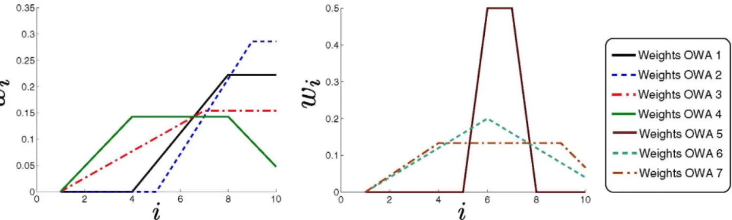
A set of aggregation functions merges all the information from (ÍQ}" r Then a set of aggregated confidence matrices {Aggj}k is generated by applying OWA operators with different weight-ing vectors. A set of seven representatives OWA operators was used, whose weighting vectors are depicted in Fig. 2. Note that the weights distributions follow trapezoidal shapes with differ-ent tilt grades. They give higher weights to the lower values of the sorted input. This way, the output of the OWA operator provides a higher confidence value when the majority of candi-dates agree. There are also null weights that correspond to the input omission.

In order to build íQ¡nai(x), we select the Aggj that best suits and less disagrees with respect to the initial {JfJjLj. In order to help

We tested the proposed method with two different data sets as it is shown in Fig. 3: (1) synthetic noise-free MR slices from the BrainWeb data set [11]; (2) one in vivo Tl MR magnitude image acquired in a GE Signa 1.5T EXCITE, FSE pulse sequence, 8 coils, TR = 500ms, TE = 13.8ms, image size 256 x 256 and FOV: 20 cm x 20 cm.

First, the synthetic images are corrupted with non-stationary noise following the model in Eq. (4). Three different spatial pat-terns, Q(x) are considered to model the spatial variation of er(x), shown in Fig. 4. The noise variance is calculated from these pat-terns for different signal-to-noise ratio (SNR) simply by a linear scaling:

CT(X) =a0 + g(x) -oi,

where er0 ar>d o\ are constants. The different patterns used are:

1. An unrealistic highly variant synthetic noise pattern, Fig. 4(a). Although it is very unlikely that a pattern like this occurs in real acquisition, this 4-section scheme will give a very good in-sight of the behavior of the filtering schemes.

2. A synthetic Gaussian-shaped noise pattern, Fig. 4(b). This pat-tern follows the shape of some real patpat-terns found in SENSE acquisitions [4,5].

0.4

•<S> 0 . 3

0.2

0.1

./•* ^£L

f

-- •

-- •

v

-Weights

-Weights

•Weights

-Weights

-Weights

-Weights

•Weights

\

OWA1

OWA 2

OWA 3

OWA 4

OWA 5

OWA 6

OWA 7 )

4 . 6 %

10

Fig. 2. Weighting quantification for the 7 OWA operators used in the paper, considering ten elements.

(a) Coronal (512 x 512) (b) Sagital (512 x 512) (c) In vivo (256 x 256)

Fig. 3. MRI slices used in the experiments. Images (a) and (b) comes from the BrainWeb data-set; (c) is a real in vivo acquisition from a multi-coil GE Signa 1.5T EXCITE.

r

0.6

L

0.2

(a) Extreme

(b)Slim

(c) SENSE

Fig. 4. Non-stationary noise patterns used with the synthetic MR images. Q(x) range is [0, 1]. It was scaled to obtain images with several SNRs.

For the experiments, a neighborhood size Ws = [7 x 7], and a

range often different central values for a2 are considered. Our

ap-proach was compared with the following state-of-the-art Rician-based filtering schemes:

• The original LMMSE estimator (Original LMMSE) as proposed in [1], assuming a single a2 value for the whole image. A 7 x 7

square window is used for the sample moments estimation. • The Non-local-mean (NLM) algorithm without the Rician bias,

as proposed in [24] (Rice NLM). The essence of the NLM algo-rithm consists on a weighted average that considers the dis-tance and intensity between the target pixel and all observed pixels. The original idea was proposed by [8] for Gaussian noise. The required parameters for this approach are the radio search window (ftsearch = 11); the radio similarity window (J?sim =3); the degreejof filtering ( / = 1.2-CT) and an estimation of the variance (a2).

• The Chi-square unbiased risk estimator (CURE), as proposed in [22]. It considers the squared-magnitude magnetic resonance image data to derive an unbiased expression for the expected mean-squared error to remove noise, which are well modeled as independent non-central chi-square random variables on two degrees of freedom. The task is done in the wavelet-domain for its compromise between the execution speed and perfor-mance. It uses the un-normalized Haar wavelet transform (Haar CURE), where each wavelet sub-band is treated independently. The other required parameter is the variance estimation, a2.

For the sake of comparison, the following methods will also be used:

- X - Noisy

- © - Ideal LMMSE

- H - Consensus

- 0 - Consensus (o-'(x))

- ^ - Original LMMSE

- # - Rice NLM

•Jf- Haar CURE

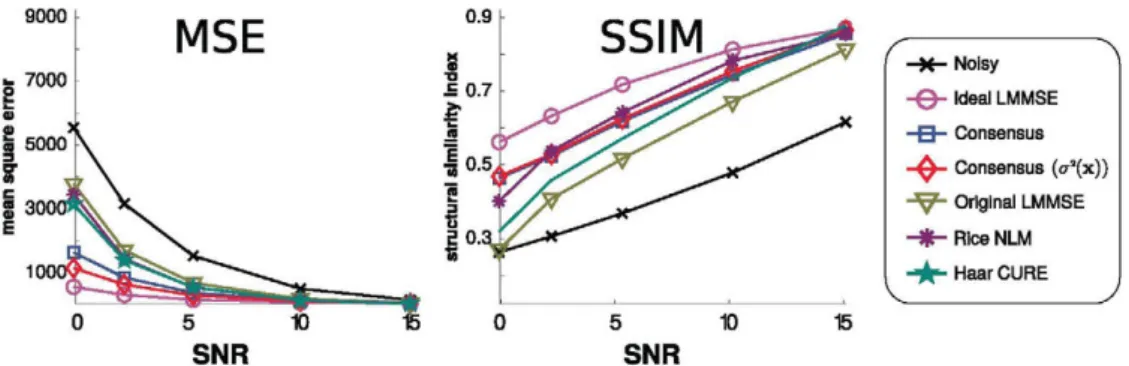
Fig. 5. Results from the first experiment: the synthetic MR magnitude image from Fig. 3(a) is corrupted with Rician noise with different SNRs generated with the noise map

in Fig. 4(a). The average of 100 realizations is considered.

upper bound of the proposal: it is the best possible solution the LMMSE can achieve.

• The LMMSE described in Eq. (5) needs an estimate of er2(x) to remove the bias of the estimated signal and a value of /<f¡nai(x) for filtering. Thus, the accuracy of the final estimated signal will depend on these two parameters. In order to isolate the behavior of the filtering and the bias reduction steps, we will show the results of the complete approach together with those in which the íQ¡nai(x) is used, but the bias is removed with the original er2(x). The former will be label as Consensus, and the latter as Consensus (a2(x)).

The restoration performance was quantified by using the Mean Square Error (MSE) and the Structural Similarity Index (SSIM) by [35]. The former measure is used to quantify the error reduction due to the filtering. It is not bounded and a higher MSE means worse quality. On the other hand, the SSIM index gives a measure of the structural similarity between the ground truth and the esti-mated image. It is bounded in [0, 1]; the closer to one, the better the image. Both measures are only applied on areas of interest in the image, this means that the background is excluded. Each ex-periment is repeated 100 times to present a significant statistical analysis.

4.2. Experiments with synthetic data

The first experiment evaluates the behavior in an extreme case with an unreal noise shape. To that end the coronal synthetic slice in Fig. 3(a) is corrupted with a non-stationary noise following the unrealistic map in Fig. 4(a). Results can be found in Fig. 5. Note that most of the methods show a poor behavior for low SNR, being the Ideal LMMSE the one with the smaller MSE and the highest SSIM. Our proposal shows also a good behavior that converges to the ideal one for high SNR. However, note that the method shows some error due to the the removal of the bias: the Consensus that uses the original er2(x) is slightly better in terms of MSE, but very similar in terms of SSIM. This means that there is some numerical error, but the underlying structure is preserved. In Fig. 6 we show a visual example for SNR = 2.21. Most of the methods works poorly on the areas with the higher noise values, but the proposal keeps the structures without any over-blur of the edges.

In the second experiment, the sagittal synthetic slice from Fig. 3(b) is corrupted with Rician noise. This time, we adopt a more realistic pattern for er(x), the slim noise map in Fig. 4(b). Due to the shape of this map, in which there is a great decay of the values of er(x) far from the center, the resulting SNR values are higher. Results for different SNRs are depicted in Fig. 7, and a visual ex-ample for SNR = 16.59 can be found in Fig. 8. Due to the higher levels of SNR, the behavior of all the filters improve, when com-pared to those of the first experiment. This time, the Consensus

Table 1

Average running times for 100 executions of the different al-gorithms and different experiments carried out.

Experiment 1 (Fig. 5) 2 (Fig. 7) 3 (Fig. 9)

Original LMMSE Consensus Haar CURE Rice NLM

0.061 ms 1.302 ms 5.828 ms 87.106 ms

0.072 ms 1.405 ms 6.710 ms 96.602 ms

0.060 ms 1.306 ms 5.727 ms 80.173 ms

approach quickly converges to the ideal value. When the SNS in-creases, CURE becomes better than to our approach. However, note that the consensus approach is limited by the selected filter, the LMMSE in this case. Nevertheless, in all the cases, our approach improves the original LMMSE with a single a value.

For the third experiment, a SENSE reconstruction is simulated from the synthetic slice in Fig. 3(a). An 8-coil system is simulated using artificial sensitivities for each coil, so that the image in the ith coil can be seen as [5]

/ , ( x ) = C , ( x ) x /0( x ) , Z = l , - . . , 8 ,

with Q(x) the sensitivity map in the /th coil. Each coil is cor-rupted with Gaussian noise with a single a value, and a correla-tion between coils is assumed {p = 0.25). The k-space is then sub-sampled by a factor 2 x and reconstructed using Cartesian SENSE. Different values of a are considered. The resulting magnitude sig-nal has a noise map similar to the one in Fig. 4(c). Results for dif-ferent SNRs are depicted in Fig. 9 while a visual example can be found in Fig. 10. This time, most of the methods show a similar behavior, with small differences between them in terms of MSE. Those differences are clearer for the SSIM index. We can clearly appreciate that CURE outperforms the rest of the approaches, fol-lowed by the NLM. Once more, note that the performance of the Consensus approach is limited by the selected filter. Note also that the case without noise estimation totally converges into the ideal one. On the other side, it is important to note that, as the SNR increases, the performance differences decrease between the algo-rithms.

Finally, we want to point out that this consensus-based ap-proach not only shows a great behavior dealing with non-stationary noise, but it also exhibits good running times. In Table 1 we present the average time of the 100 executions considered for each algorithm.1 Not that the original LMMSE is a very fast method, closely followed by our approach. On the other hand, the Rice NLM obtains high running times with respect to the rest of the filters. This issue must be taken into account if the filters are going to be used in large data sets.

(a) Noisy (b) CURE (c) Rice NLM (d) Consensus

MSE=3174, SSIM=0.31 MSE=1410, SSIM=0.46 MSE=1440, SSIM=0.54 MSE=874, SSIM=0.52

Fig. 6. Visual results of the Altered image obtained from the synthetic MR magnitude image from Fig. 3(a) with the extreme noise map in Fig. 4(a), with a SNR = 2.21.

250

- K - Noisy

- © - Ideal LMMSE

- Q - Consensus

- A - Consensus (o"!(x)) - ^ - Original LMMSE

- * - Rice NLM

•+- Haar CURE

J

17 18

SNR

Fig. 7. Results from the second experiment: the synthetic sagittal MR magnitude slice from Fig. 3(b) is corrupted with Rician noise with different SNRs generated with the em slim noise map in Fig. 4(b). The average of 100 realizations is considered.

(a) Noisy (MSE = 135.74, SSIM = 0.66) (b) CURE (MSE = 48.86, SSIM = 0.87)

(c) Rice NLM (MSE = 67.97, SSIM = 0.84) (d) Consensus (MSE=40.02, SSIM = 0.88)

MSE

10 12 14 16

SNR

18 20

SSIM

12 14 16

SNR

18 20 22

- H - Noisy

- © - Ideal LMMSE

- B - Consensus

• A - Consensus (CT'(X))

- ^ - Original LMMSE

- * - Rice NLM

- ^ - Haar CURE

Fig. 9. Results from the third experiment: the synthetic sagittal MR magnitude slice from Fig. 3(b) is used to simulate a SENSE reconstruction with different SNRs. The

average of 100 realizations is considered.

(a) Noisy ( M S E = 141, S S I M = 0.59) (b) CURE ( M S E = 27, SSIM = 0.93)

(c) Rice NLM ( M S E = 58, SSIM = 0.88) (d) Consensus ( M S E = 42, SSIM = 0.88)

Fig. 10. Visual results of the Altered image obtained from a SENSE image, generated from the synthetic MR magnitude image from Fig. 3(a), with a SNR = 15.66. An 8-coil

system is considered.

4.3. Experiments with real data

Finally, in order to test the proposed method with real data, we use the multi-coil in vivo acquisition in Fig. 3(c). For simplicity, the fully sampled k-space has been acquired, and the sensitivity map has been estimated for each of its 8 coils. The data in each coil was sub-sampled to simulate a 2 x acceleration, and the final magnitude image has been reconstructed using an offline SENSE algorithm. Since the initial er2(x) is not available for this image, a prior estimation is done assuming stationary noise [1] as

(T2=mode{(JVi(x)2>x}.

The Wm)m=i elements are selected from the range 1% to 103% of the estimated a, that is, the interval [0.0001 -a2, , 1.0609 - a2] . Since there is no golden standard available for comparison, we only

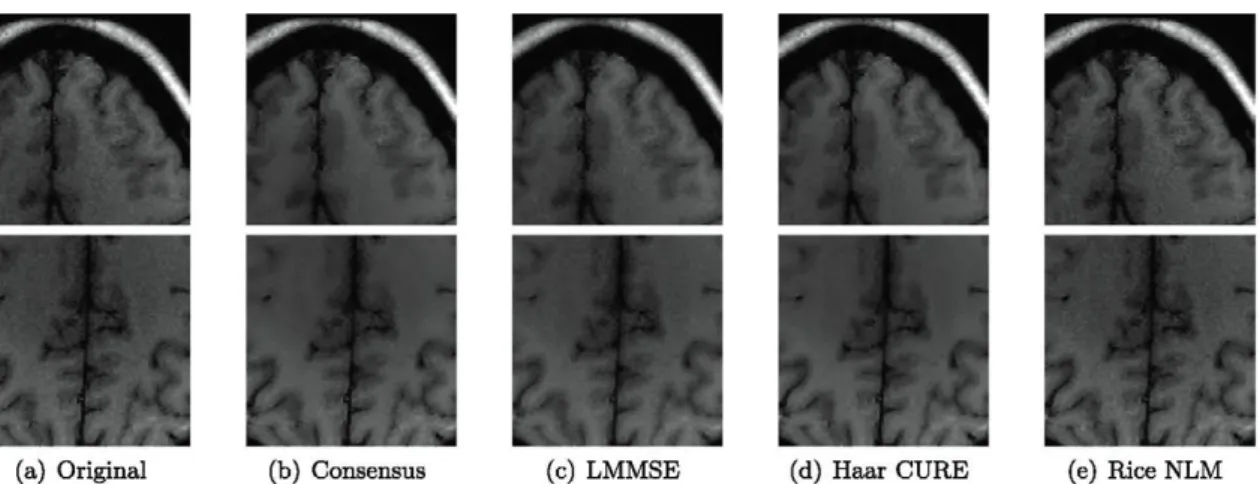
show visual results in Fig. 11 for the different filters considered. The consensus LMMSE and the Haar CURE obtain the best results among the restored images, although consensus LMMSE slightly obtains better results in homogeneous areas. On the other hand, the restored Rice NLM image still keeps some noisy pattern, while the original LMMSE over-filter the data, producing some blur (this effect is emphasized close to the borders).

5. Conclusions

•

(a) Original (b) Consensus (c) LMMSE (d) Haar CURE (e) Rice NLM

Fig. 11. Visual results for the in vivo data set in Fig. 3(c): details from the Altered images.

clearer example of this kind of noise in MR data can be found in pMRI acquisitions, but not only. The proposed method is applied together with some existing filtering method. In this paper, the LMMSE signal estimator for stationary Rician noise is considered. This filter on its own will fail when applied over a spatially variant cr2(x), since it is intended for a single a2. However, the

combina-tion of the LMMSE with the proposed consensus approach is able to take into account the non-stationarity of the data. The algorithm also assumes our incapability to proper estimate the input data, in this case the map of noise and the optimal size of the window in which the local moments are calculated.

Results of the experiments done using synthetic and real data show how the proposed method highly improves the behavior of the stationary LMMSE, and its performance is very similar to the optimal case assuming a non-stationary LMMSE with er2(x) per-fectly known. In many cases, the new approach even outperforms Rician filters that in the past have shown even a better perfor-mance than the LMMSE itself. The method is particularly useful in those cases when the variability of er2(x) is high and extreme. That will depend on the position and calibration of the acquisition coils.

As we have previously stated, this philosophy of work can be easily extended to other filtering techniques in MRI. This exten-sion will allow other algorithms to better cope with non-stationary noise, but not only. They can also be adapted to automatically se-lect the better set of input parameters, or to cope with deviation from the statistical model, to perform a different filtering around important structures and edges or even to combine the results of different kind of filters into a single output.

The main drawback of the method is that the number of oper-ations increases, since the method carries out a filtering procedure for each input set. The more the input possibilities, the greater the number of times the filtering is repeated. The good news here is that each of the iterations is totally independent of the others, and therefore the method can easily be highly parallelized.

Acknowledgements

This work was supported by European Commission under Con-tract no. 238819 (MIBISOC Marie Curie ITN) and Ministerio de Ciencia e Innovación for grant TEC2013-44194. The authors also ac-knowledge Centro de Técnicas Instrumentales, Universidad de Val-ladolid and Doctor W. Scott Hoge from Brigham and Womens Hos-pital, Boston for MRI acquisitions. Gonzalo Vegas-Sánchez-Ferrero acknowledges Consejería de Educación, Juventud y Deporte of Co-munidad de Madrid and the People Programme (Marie Curie

Ac-tions) of the European Union's Seventh Framework Programme (FP7/2007-2013) for REA grant agreement no. 291820.

References

[1] S. Aja-Fernández, C. Alberola-López, C.-F. Westin, Noise and signal estimation

in magnitude MRI and Rician distributed images: a LMMSE approach, Image Process., IEEE Trans. 17 (8) (2008) 1383-1398.

[2] S. Aja-Fernández, T. Pieciak, G. Vegas-Sanchez-Ferrero, Spatially variant noise

estimation in MRI: a homomorphic approach, Med. Image Anal. 20 (2015) 184-197.

[3] S. Aja-Fernández, A. Tristán-Vega, C. Alberola-López, Noise estimation in

sin-gle- and multiple-coil magnetic resonance data based on statistical models, Magn. Reson. Imaging 27 (10) (2009) 1397-1409.

[4] S. Aja-Fernández, G. Vegas-Sanchez-Ferrero, Statistical analysis of noise in MRI,

Springer Science, Switzerland, 2016.

[5] S. Aja-Fernández, G. Vegas-Sánchez-Ferrero, A. Tristán-Vega, Noise estimation

in parallel MRI: GRAPPA and SENSE, Magn. Reson. Imaging 32 (3) (2014) 281-290.

[6] G. Beliakov, S.James, A penalty-based aggregation operator for non-convex

in-tervals, Knowl. Based Syst. 70 (2014) 335-344.

[7] P. Borrelli, G. Palma, M. Comerci, B. Alfano, Unbiased noise estimation and

de-noising in parallel magnetic resonance imaging, in: IEEE International Confer-ence Acoustics, Speech and Signal Processing (ICASSP), 2014, pp. 1230-1234.

[8] A. Buades, B. Coll, J.M. Morel, A review of image de-noising algorithms, with a

new one, Multi-scale Model. Simulation 4 (2) (2005) 490-530.

[9] T. Calvo, G. Beliakov, Aggregation functions based on penalties, Fuzzy Sets Syst.

161 (10) (2010) 1420-1436.

[10] T. Calvo, R. Mesiar, R.R. Yager, Quantitative weights and aggregation, Fuzzy

Syst. IEEE Trans. 12 (1) (2004) 62-69.

[ 11 ] C.A. Cocosco, V. Kollokian, R.K.-S. Kwan, G.B. Pike, A.C. Evans, Brainweb: online interface to a 3D MRI simulated brain database, Neurolmage, volume 5, 1997.

[12] I. Delakis, O. Hammad, R.I. Kitney, Wavelet-based de-noising algorithm for

im-ages acquired with parallel magnetic resonance imaging (MRI), Phys. Med. Biol. 52 (13) (2007) 3741.

[13] O. Dietrich, J.G. Raya, S.B. Reeder, M. Ingrisch, M.F. Reiser, S.O. Schoenberg,

In-Auence of multichannel combination, parallel imaging and other reconstruc-tion techniques on MRI noise characteristics, Magn. Reson. Imaging 26 (6) (2008) 754-762.

[14] L. González-Jaime, E.E. Kerre, M. Nachtegael, H. Bustince, Consensus image

method for unknown noise removal, Knowl. Based Syst. 70 (2014) 64-77.

[15] L, González-Jaime, M. Nachtegael, E.E. Kerre, G. Vegas-Sánchez-Ferrero,

S. Aja-Fernández, Parametric image restoration using Consensus: an applica-tion to nonstaapplica-tionary Noise Altering, in: J.M. Sanches, L. Mico, J.S. Cardoso (Eds.), Pattern Recognition and Image Analysis, Lecture Notes in Computer Sci-ence, volume 7887, Springer Berlin Heidelberg, 2013, pp. 358-365.

[16] B. Goossens, A. Pizurica, W. Philips, Wavelet domain image denoising for

non-stationary noise and signal-dependent noise, in: IEEE International Con-ference on Image Processing, 2006, pp. 1425-1428.

[17] M.A. Griswold, P.M. Jakob, R.M. Heidemann, M. Nittka, V. Jellus, J.M. Wang,

B. Kiefer, A. Haase, Generalized autocalibrating partially parallel acquisitions (GRAPPA), Magn. Reson. Med. 47 (6) (2002) 1202-1210.

[18] H. Gudbjartsson, S. Patz, The Rician distribution of noisy MRI data, Magn.

Re-son. Med. 34 (6) (1995) 910-914.

[19] R.M. Henkelman, Measurement of signal intensities in the presence of noise in

MR images, Med. Phys. 12 (2) (1985) 232.

[20] J.-P. Liu, S. Lin, H.-Y. Chen, C¿. Xu, Penalty-based continuous aggregation

[21] R.W. Liu, L. Shi, W. Huang, J. Xu, S.C.H. Yu, D. Wang, Generalized total varia-tion-based MRI Rician de-noising model with spatially adaptive regularization parameters, Magn. Reson. Imag. 32 (6) (2014) 702-720.

[22] F. Luisier, T. Blu, P.J. Wolfe, A CURE for noisy magnetic resonance images:

chi-square unbiased risk estimation, Image Process. IEEE Trans. 21 (8) (2012) 3454-3466.

[23] M. Maggioni, A. Foi, Nonlocal transform-domain de-noising of volumetric data

with group-wise adaptive variance estimation, IS&T/SPIE Electronic Imaging, International Society for Optics and Photonics, 2012. 82960O-82960O-8

[24] J.V. Manjon, J. Carbonell-Caballero, J.J. Lull, G. Garcia-Marti, L Marti-Bonmati,

M. Robles, MRI de-noising using Non-Local Means, Med. Image Anal. 12 (4) (2008) 514-523.

[25] J.V. Manjon, P. Coupe, A. Buades, MRI noise estimation and de-noising using

non-local PCA, Med. Image Anal. (2015).

[26] G. McGibney, M.R. Smith, An unbiased signal-to-noise ratio measure for

mag-netic-resonance images, Med. Phys. 20 (4) (1993) 1077-1078.

[27] X. Pan, X. Zhang, S. Lyu, Blind local noise estimation for medical images

recon-structed from rapid acquisition, in: SPIE Medical Imaging, 2012, p. 83143R.

[28] T. Pieciak, G. Vegas-Sánchez-Ferrero, S. Aja-Fernández, Variance stabilization of

noncentral-chi data: application to noise estimation in MRI, Biomedical Imag-ing: From Nano to Macro, 2016 IEEE International Symposium on, 2016.

[29] K.P. Pruessmann, M. Weiger, M.B. Scheidegger, P. Boesiger, SENSE: sensitivity

encoding for fast MRI, Magn. Reson. Med. 42 (5) (1999) 952-962.

[30] P.M. Robson, A.K. Grant, A.J. Madhuranthakam, R. Lattanzi, D.K. Sodickson,

C.A. McKenzie, Comprehensive quantification of signal-to-noise ratio and g-factor for image-based and fi-space-based parallel imaging reconstructions, Magn. Reson. Med. 60 (4) (2008) 895-907.

[31] J. Sijbers, A.J. den Dekker, P. Scheunders, D. Van Dyck, Maximum-likelihood

estimation of Rician distribution parameters, Med. Imaging, IEEE Trans. 17 (3) (1998) 357-361.

[32] K. Tabelow, H.U Voss, J. Polzehl, Local estimation of the noise level in MRI

using structural adaptation, Med. Imag. Anal. 20 (1) (2015) 76-86.

[33] P. Thunberg, P. Zetterberg, Noise distribution in SENSE- and

GRAPPA-recon-structed images: a computer simulation study, Magn. Reson. Imaging 25 (7) (2007) 1089-1094.

[34] A. Tristán-Vega, V. García-Pérez, S. Aja-Fernández, C.F. Westin, Efficient and

ro-bust nonlocal means de-noising of MR data based on salient features match-ing, Comput. Methods Prog. Biomed. 105 (2) (2012) 131-144.

[35] Z. Wang, A.C. Bovik, H.R. Sheikh, E.P. Simoncelli, Image quality assessment:

from error visibility to structural similarity, Image Process. IEEE Trans. 13 (4) (2004) 600-612.

[36] R.R. Yager, On ordered weighted averaging aggregation operators in