Comparison
of
airborne
laser
scanning
methods
for
estimating
forest
structure
indicators
based
on
Lorenz
curves
Rubén
Valbuena,
Jari
Vauhkonen
,
Petteri
Packalen,
Juho
Pitkänen,
Matti
Maltamo
a b s t r a c t
Thepurposeofthisstudywastocompareanumberofstate-of-the-artmethodsinairbornelaserscan-ning(ALS)remote sensingwithregardstotheircapacitytodescribetreesizeinequalityandotherindi-catorsrelatedtoforeststructure.The indicatorschosenwerebasedontheanalysisoftheLorenzcurve:Ginicoefficient(GC),Lorenzasymmetry(LA),theproportions ofbasalarea(BALM)andstemdensity(NSLM)stockedabovethemeanquadraticdiameter.Eachmethodbelongedtooneof theseestimationstrategies:(A)estimatingindicatorsdirectly;(B)estimatingthewholeLorenzcurve;or(C)estimatinga completetreelist.Acrossthesestrategies,themostpopularstatisticalmethodsforarea-basedapproach(ABA)wereused: regression,randomforest(RF),andnearestneighbourimputation.ThelatterincludeddistancemetricsbasedoneitherRF (NN–RF)ormostsimilarneighbour(MSN).Inthecaseoftreelistesti-mation,methodsbasedonindividualtreedetection(ITD) andsemi-ITD,bothcombinedwithMSNimpu-tation,werealsostudied.Themostaccuratemethodwasdirectestimationby bestsubsetregression,whichobtainedthelowestcross-validatedcoefficientsofvariationoftheirrootmeansquarederror CV(RMSE)formostindicators:GC(16.80%),LA(8.76%),BALM(8.80%)andNSLM(14.60%).Similarfigures[CV(RMSE)16.09%, 10.49%,10.93%and14.07%,respectively]wereobtainedbyMSNimputationoftreelistsbyABA,amethodthatalsoshoweda numberofadditionaladvantages,suchasbetterdistributingtheresidualvariancealongthepredictiverange.Inlightofour results,ITDapproachesmaybeclearlyinferiortoABAwithregardstodescribingthestructuralpropertiesrelatedtotreesize inequalityinfor-estedareas.
1. Introduction
Indicators describing forest structure can be a valuable support tool in decision-making and forest management planning. Maps of forest structure indicator estimates can be used as a reference to evaluate the success of regeneration groups, plan the location of the next selective cuttings or evaluate the need for thinning (Burger, 2009). Because of its complete three-dimensional
charac-terization of vegetation, airborne laser scanning (ALS) remote
sensing allows for evaluating properties related to forest structure
in broad forest areas (Lefskyetal.,2005;Maltamoet al.,2005).
These properties can be exploited to study forest successional
stages(Falkowskietal.,2009;Valbuenaetal.,2013a),theriskof
wild fire propagation (Andersenetal.,2005;Halletal.,2005) or
wind-throwdamage(Suárezetal.,2008),orcharacteristicsrelated
tohabitatquality(Lefskyetal.,2002;Martinuzzietal.,2009).
LexerødandEid(2006)pointed out a number of motivations for
using indicators derived from Lorenz curves to describe forest
structure.Inaforest,theLorenzcurveexpressesdominance
rela-tions by comparing relative cumulated proportions of basal area
and stem density accounted for each tree (Valbuenaetal.,2012).
Ginicoefficient(GC), Lorenzasymmetry (LA), the proportions of
basalarea(BALM)andstemdensity(NSLM)stockedabovethe
which have been suggested for describing tree size inequality and
the balance among forest subpopulations. TheGChas been
demon-strated to more reliably describe tree size distributions than other indicators based on product moments (Knox et al., 1989) or
infor-mation theory (Valbuena et al., 2012). For this reason,Bollandsås
and Næsset (2007) and Duduman (2011)usedGCas a basis to
dis-criminate among differently-shaped diameter distributions. TheGC
is the ratio between the second and first L-moments, and therefore a second order descriptor of concentration, i.e. relative dispersion (Hosking, 1990). The attention has recently been turned to study-ing tree size inequality by L-moments, especially with regards to their relations with ALS datasets (Ozdemir and Donoghue, 2013; Valbuena et al., 2013b). Furthermore, the coefficient ofLA
devel-oped by Damgaard and Weiner (2000) was employed by
Valbuena et al. (2013a) for characterizing the relation between
dominant and subdominant cohorts in multi-layered forests.LA
is a join description ofBALMandNSLM, two important structural
characteristics of forests closely related to one another. In forestry
practice,BALM and NSLMhave traditionally applied when using
structural stocking guides in decision-making (Gove, 2004). Previous research aiming at estimating these indicators from ALS were mainly based on parametric modelling, including best subset (Valbuena et al., 2013b) and beta regression (Valbuena et al., 2013a). Most difficulties were found in the variance structure observed on the prediction, and also on the complexity of the
rela-tion ofLAwith ALS metrics. These issues may be solved when using
non-parametric approaches based on nearest neighbour
imputa-tion (k-NN).Maltamo et al. (2006) and Hudak et al. (2008)outlined
a number of advantages in using non-parametric procedures, which can make them preferable depending on each application. The method of most similar neighbour (MSN) imputation has already
become operational for ALS-estimation of forest variables
(Maltamo and Packalen, 2014). Based on a canonical correlation
analysis, MSN imputes thekmost similar relations of covariability
between response and predictors found within the training dataset (Moeur and Stage, 1995). Furthermore, random forest (RF) is also becoming increasingly popular in ALS remote sensing (Falkowski et al., 2009; McInerney et al., 2010; Yu et al., 2011). RF consists in bootstrapping the training data and computing a regression tree at each iteration, i.e. recursive partitioning by a succession of binary splits of predictor thresholds determined under the criterion of residual sum of squares minimization (Hastie et al., 2009). A
com-bination of RF andk-NN is an approach where a distance metric
used ink-NN is determined based on RF proximity matrix (NN–
RF) (Crookston and Finley, 2008).Hudak et al. (2008)found NN–
RF to be more robust than other nearest neighbour methods for imputing species-specific basal area and stem densities. We there-fore hypothesised that a similar outcome may be obtained for Lor-enz curve descriptors, as they simultaneously describe the relations between basal area and stem density (Valbuena et al., 2012).
These methods can be employed with the purpose of obtaining the estimation of a complete tree list, an alternative which may be beneficial when the interest is on knowing the shape of the diameter distribution, for instance in complex multilayered forest structures. Bollandsås and Næsset (2007)used an area-based approach (ABA) with partial least squares regression to estimate discrete quantiles
along the diameter distribution, using theGCas a basis for stratifying
the dataset into homologous diameter distribution types. Alterna-tively, estimating Weibull model parameters allowed inferring diameter distributions presenting a wide range of simple shapes without prior stratification (Gobakken and Næsset, 2004; Maltamo et al., 2007).Maltamo et al. (2006)introduced the use of MSN impu-tation in ALS estimation, later including the impuimpu-tation of discrete quantiles (Packalén and Maltamo, 2008), which tolerated the use of complex diameter distribution shapes without theoretical param-eterization. Both diameter and basal area-weighted distributions
have been estimated with the intention of improving ALS prediction of forest variables (Gobakken and Næsset, 2004; Maltamo et al., 2007). However, no previous research has been devoted to applying this method on the Lorenz curve, which is a joint description of the intrinsic relation between a diameter distributions and its basal area-weighted (Gove and Patil, 1998; Valbuena et al., 2012).
Individual tree detection (ITD) methods have also traditionally been a source for supplying tree lists. ITD methods are based on seg-mentation of individual tree crowns from a canopy height model (CHM). The performance of the ITD algorithms typically depends on tree density and spatial distribution of trees, i.e. clustering pat-terns (Vauhkonen et al., 2012). They usually have the disadvantage of underestimating the understory, although this may not matter for estimating many important forest parameters such as basal area or volume (Persson et al., 2002; Pitkänen et al., 2004). More informa-tion on the understory may be obtained with improved tree detec-tion algorithms (Lähivaara et al., 2013), direct point cloud segmentation (Li et al., 2012), using full-waveform ALS information (Reitberger et al., 2009), or analyzing combined leaf-on and leaf-off acquisitions in deciduous forests (Hill and Broughton, 2009). Maltamo et al. (2004), Lindberg et al. (2010), Vauhkonen et al. (2010) and Vastaranta et al. (2012)combined ABA and ITD with the purpose of overcoming this difficulty and improving estimation
accuracy. Moreover,Breidenbach et al. (2010)introduced the idea of
semi-ITD, in which all trees measured inside a given segment are considered to be represented by that segment, and not just the dom-inating tree. All these methods have been commonly evaluated by means of the improvement obtained in total forest estimates.
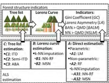
In this article we compare these state-of-the-art ALS estimation methods, with the objective of evaluating them with regards to their capacity for assessing characteristics of forests related to tree size inequality, and the balance between overstory and understory layers. Indicators derived from the study of the Lorenz curve were selected for this purpose, further clarifying their relations with ALS metrics. We compared the results obtained with three different estimation strategies consisting of: (A) direct indicator estimation; (B) non-parametric estimation of the Lorenz curve, and posterior indicator derivation; or (C) estimating a complete tree list, from which the Lorenz curve and derived indicators were later derived (Fig. 1). Many different methods were tested for each strategy, with the purpose of selecting the most appropriate methodological combination for this type of forest structure-related response.
2. Materials and methods
2.1. Study area and remote sensing predictors
The study was carried out in 800 ha of forest situated at the municipality of Kiihtelysvaara in the province of North Karelia
(Finland; approx. lat.: 62°310N; lon.: 30°100E; 130–150 m above
sea level). Main tree species in the area were Scots pine (Pinus
syl-vestrisL.) and Norway spruce (Picea abies(L.) Karst.), with a minor proportion of broadleaved species. The ALS data were acquired on 26 June 2009, using an ALTM Gemini sensor (Optech, Canada). The flight was performed at a height of about 600 m above terrain level
with a maximum scanning angle of 26°, rendering a 320 m swath
width with a 55% side lap between strips. A pulse repetition rate of 125 kHz, yielded a high-resolution dataset with nominal scan
density of 11.9 pulses m2. Returns we classified as ground by
iter-atively filtering lower returns into a Delaunay-triangulated
irregu-lar network (c.f.Axelsson, 2000). Ground points were interpolated
into a digital terrain model (DTM) of 0.5-m pixel size.
By subtracting the DTM value beneath each individual ALS echo, their altitudes above ground level were obtained as a prior step for predictor computation. ALS predictors were moment, order and quantile statistics (Magnussen and Boudewyn, 1998), L-moments and their ratios (Hosking, 1990) and canopy cover metrics (McGaughey, 2012) computed from these ALS echo altitudes. This set of predictors was generated with the assistance of software FUSION (version 3.1, USDA Forest Service), and statistical analyses were carried out in R environment (R Development Core Team, 2011). The initial predictor dataset was reduced using least absolute
shrinkage and selection operator (LASSO;Hastie et al., 2009), as
detailed inValbuena et al. (2014). As common in ABA methods,
the same metrics were used to estimate them at plot level, for model training, and over a grid of cells covering the whole ALS surveyed area, for wall-to-wall prediction of the target response (Næsset, 2002).
2.2. Lorenz curve and forest structure indicators
Field survey was completed between May and June 2010, and consisted of stratified sampling with a total of 79 squared plots whose positions were subjectively determined to assure full cover-age of variability range in the forest response. Plot size was either
2020, 2525 or 3030 m, varying in relation to stem density
for practical purposes. The forest mensuration campaign
deter-mined diameter at breast height (dbhi, cm) with a calliper, tree
height (hi, m) with a Vertex hypsometer (Haglöf UAB, Sweden),
and species (spi, dummy variable), for every individual tree (i)
within plot with eitherdbhi P 5 orhi P 4. Stem volumes (
v
i,m3) were obtained as detailed by Vauhkonen et al. (2014). The
position of every individual tree recorded in the field was deter-mined in relation to the ALS dataset, using the least squares
method described byKorpela et al. (2007). Basal areas were
calcu-lated for single stems (bai, m2), and quadratic mean diameters
computed at plot level (QMD, cm) as thedbhwhich corresponds
to the mean basal area (ba, m2). By ordering the individual trees
in ranks (r) of decreasingdbh, the Lorenz curves were computed
at plot level as the cumulative proportion of the total basal area
M(xr) in relation to the cumulative proportion of stem densityxr
accounted from each of them (Valbuena et al., 2012). The indica-tors of forest structure were all based on this Lorenz curve, using
the rationale detailed byValbuena et al. (2013b).
The first indicator of forest structure wasGC, i.e. the Gini
coef-ficient of the plot leveldbhdistribution, also called L-coefficient of
variation (Hosking, 1990). The second indicator wasNSLM, the
pro-portion of number of stems which are larger than the weighted
mean (QMD). In other words,NSLMis the share of stem density
stocked above theQMD, which is the value of the Lorenz plot’sx
-axis at the inflexion point of the curve xQMD (Valbuena et al.,
2013a). The third indicator was the corresponding value for the
y-axisM(xQMD), which is the proportion basal area larger than the
QMD(BALM;Gove, 2004). It was also considered to average the lat-ter two indicators into a single one describing the skewness of the
Lorenz curve. A fourth indicator of Lorenz asymmetry (LA) was
therefore computed, using the concept developed for forestry by Valbuena et al. (2013a)as modified version of the original indicator
designed byDamgaard and Weiner (2000).
It is noteworthy to reflect on the properties of these indicators, with the intention of assisting the readers in interpreting the results of this study. The dependent variables considered are dimensionless indices and proportions, and therefore they all the-oretically range [0, 1]. However, this range is in practice limited a
number of factors. For instance, the upper limit atGC= 1
(mathe-matically provided by a maximally bimodal distribution), corre-sponds to a forest situation which is likely to be ecologically implausible (Valbuena et al., 2013a). Moreover, the quadratic
rela-tion betweendbhiandbaiimposes a finite lower limit to theQMD,
and therefore to the probability density of the basal area-weighted distributions (Gove and Patil, 1998). As a result, the theoretical
range of values for BALMandNSLM is in practice much shorter.
For instance,Gove (2004)demonstrated thatBALMhas a maximum
range between [0.58, 0.99] for anydbhdistribution conforming to a
Weibull function, which is a common condition for real forests. A
similar situation occurs forNSLM, as some probability density must
always be above theQMD, and the position of the Lorenz curve’s
inflexion cannot range the whole extent of thex-axis in practice.
Furthermore,Valbuena et al. (2013b)reflected on the inverse
rela-tion between BALM and NSLM, which makes them cancel each
other out in their averagedLAindicator, therefore further reducing
the plausible range of values forLA.
2.3. Strategies for ALS estimation of Lorenz indicators
With the purpose of predicting the described indicators of forest structure by means of ALS remote sensing, a number of approaches were followed and compared. They all may be grouped in three main types of strategies, as each of them obtained the predictions by either (A) estimating the target indicators directly, (B) estimat-ing the whole Lorenz curve, or (C) estimatestimat-ing a full tree list (Fig. 1). All these approaches are intrinsically related, as the Lorenz curve
expresses the quadratic relationship between thedbhdistribution
and its area-based weighted counterpart (Gove and Patil, 1998). In strategy A, ALS metrics were related with each response variable
yA= (GC,LA,BALM,NSLM) at plot level. Strategy B consisted in
estimating regular quantiles along the whole Lorenz curveyB=
{-M(.05),M(.10),. . .,M(.90),M(.95)}, and use them for deriving the
same indicators afterwards. BeingM(xr) the Lorenz curve of trees
ordered by decreasing sizes, M(.05) is the relative proportion of
the total basal area which is stocked in the 5% largest trees,
M(.10) is for the largest 10%, etcetera. Furthermore, methods
fol-lowing strategy C yielded an estimation along the wholedbh
fre-quency distribution at discrete 1 cm-wide diameter classes. In
other words, yC= {Ndbh=1,Ndbh=2,. . .,Ndbh=50,Ndbh=51} where Ndbh=i
was the proportion in number of stems for the diameter classi.
The same Lorenz-based indicators were also generated at plot level from these estimated tree lists, and therefore the final outcome of any of these approaches was a final estimate for each indicator
^
y¼GCc;LAc;BALMd ;NSLMd : ð1Þ
All the methods considered were compared by means of their capacity for reliably predicting the targeted final indicators of
computed for each plotj= 1, 2,. . .,mfrom the field data. The
pre-dicted indicators y^j¼ GCdj;LAcj;BALMdj;NSLMdj
were all obtained in a leave-one-out cross validation (LOOCV) fashion, as detailed
for each method. Each of these target indicatorsy^jwere also
gen-erated from the outcome of those methods aiming at deriving
either a Lorenz curve (B) or adbh distribution (C), following the
same approach as for the field data. In other words, for the purpose of this study we focused on the capacity of the methods to detect
properties related to dbh inequality, regardless of their capacity
fordbhestimation itself. LOOCV procedures involved, in all cases,
the full process of indicator generation: training, including both distance metric calculation and imputation (Packalén et al., 2012), and also tree list and Lorenz curve generation. The
discrep-ancy between the observed (yj) and predicted (y^j) values could
therefore be evaluated by their mean difference (bias), and also by their root mean squared error (RMSE). By dividing by the observed mean values, we also obtained relative figures for the bias (bias%), and also the coefficient of variation of the RMSE
[CV(RMSE)%]. Coefficients of determination (R2) were also
employed to compare the relation betweenyjandy^j, from the sums
of squares ratio between residualsðyjy^jÞand the total observed
varianceðyjyjÞ.
Many different estimation methods were tested for each of these strategies (Fig. 1). The ABA method was employed across all strategies, in the sense of relating ALS metrics at plot level. Best subset regression method based on the linear model (LM) was selected as parametric approach for direct indicator estimation.
Non-parametric approaches included random forest (RF) and k
-NN methods. For the latter, two types of distance metrics were considered when computing the nearest neighbours. The most similar neighbour (MSN) method, which computes the distance based on canonical correlation, was the first type. On the other hand, the second type was based on using the RF algorithm for computing the distance metric in the imputation (NN–RF). Finally, MSN imputation was the statistical method involved in all approaches following the strategy C of full tree list estimation, though the reference response differed in each case, as detailed below. Another important difference is that imputation in ABA was done at plot level, whereas in ITD and semi-ITD it was carried out the scale tree crowns (segment level).
2.3.1. Area-based approaches (ABA)
2.3.1.1. Best subset linear model (LM). Best subset regression was
carried our following the methodology described by Valbuena
et al. (2013b) for a different study area. A set of models was obtained containing all plausible combinations with a number of p= 1,. . ., 5 predictors. The best model was therefore selected under the criterion of lowest Akaike information criterion, using the
ver-sion corrected (AICc) for finite samples bySugiura (1978). This
pro-cedure was carried out separately for each response variable
y= (GC,LA,BALM,NSLM). Accuracy assessment was carried out by
LOOCV, so that an estimate for each plot j was obtained after
removing it from the training dataset.
2.3.1.2. Random Forest (RF). Boosted recursive partitioning was
car-ried out with the packagerandomForest(version 4.6-7;Liaw and
Wiener, 2002). The RF iterations were fitted by regression, so that the variable and threshold for dichotomous split at each node were selected under the criterion of minimum residual sum of squares. All plausible candidate predictors were boosted, i.e. randomly per-muted, at each node of the tree. New additive terms (tree branches) kept growing recursively according to an exponential loss function (Hastie et al., 2009). A 0.2 fraction of the remaining predictors was excluded at each iteration, and the out-of-bag error, i.e. the residual measured against the samples that did not appear at each bootstrap, was estimated for the resulting RF. This
successive branching iterated until this out-of-bag error became smaller than the standard error of the minimum error rate of all forests. As a result, each forest consisted of 500 regression trees form which their mode is selected for the final RF imputation, or a random selection from equal modes in case of ambiguity. Accu-racy assessment was carried out by LOOCV as well, so that a new
RF was trained from each subset after removing one plotj.
2.3.1.3. Methods based on k-NN imputation. Nearest neighbour methods, i.e. estimation based on computing statistical distance metrics to reference sample plots, were carried out with the pack-age yaImpute (version 1.0-18; Crookston and Finley, 2008). The
choice of the optimalkis a compromise between bias and precision
in the estimation (Eskelson et al., 2009). We decided to setk= 3,
after observing the evolution of a LOOCV RMSE for increasingk.
The final imputed value was a weighted average of theknearest
neighbours, according to their distance in the feature space. Accu-racy assessment was also done by LOOCV, computing new
canon-ical vectors after removing each plotj, to avoid its potential effect
on the canonical correlation itself (Packalén et al., 2012).
The distance metric used in nearest neighbour determination was calculated following two methods: the random forest algo-rithm (NN–RF) and the canonical correlation components (MSN). Either method consists in transforming the feature space, i.e. the predictor dataset, with the purpose of maximizing the explained variability against the given response. In order to allow direct com-parison, algorithm parameters in NN–RF remained unchanged
from those described for RF. PackagerandomForestwas therefore
used withinyaImpute(methodrandomForest). BeingyBa
multivar-iate response, in practice this implies a modification of the RF algo-rithm for computing a separate random forest for each segment of the Lorenz curve (Crookston and Finley, 2008). Then, the imputa-tion in NN–RF was done based on the RF proximity matrix. In MSN, on the other hand, the imputation was done based on the canonical correlation components (Moeur and Stage, 1995). In Lor-enz curve estimation, components are computed for the multivar-iate response a whole (Valbuena et al., 2014). The weighted
average of thekmost similar neighbours was computed according
to their distance in the projected canonical correlation space (Packalén and Maltamo, 2008).
The use of canonical correlation analysis to calculate the dis-tance metric for imputation makes the MSN method well suited to situations requiring a multivariate response (Packalén et al., 2012). For this reason, Packalén and Maltamo (2008) included the complete tree list as reference dataset during the imputation,
in order to obtain discrete estimates along the wholedbh
distribu-tion. In this study, we considered the possibility for computing the target forest structure indicators from a MSN-estimated complete list (this method is denoted as ABA withing those in strategy C). Thus, the MSN method for ABA estimation was employed across all strategies, and therefore the difference laid on the response
being imputed from the neighbours (yA,yBoryC). BeingyCa large
number of dependent variables that would leave insufficient degrees of freedom for canonical correlation analysis, it was used for imputation stage while the components themselves where
computed with y= (GC,LA,QMD), as these can suffice to obtain
accurate predictions of diameter distributions (Maltamo et al., 2009).
2.3.2. Individual tree detection (ITD) and semi-ITD (S-ITD)
Table 1
Accuracy assessment results for estimation methods based on the strategy of (A) direct indicator estimation (seeFig. 1). LM: linear regression model (A1); RF: random forest (A2); NN–RF: nearest neighbour based on RF (A31); MSN: most similar neighbour (A32).
Method Gini coefficient (GC) Lorenz asymmetry (LA)
RMSE CV(RMSE)% Bias Bias% RMSE CV(RMSE)% Bias Bias%
A1: LM 0.076 16.80 5.56104
0.12 0.053 8.76 6.45105
0.01
A2: RF 0.105 23.44 1.57103 0.35 0.056 9.27 7.40
104 0.12
A31: NN–RF 0.130 28.81 1.03101
2.28 0.066 10.87 5.00104 0.08
A32: MSN 0.100 22.16 5.10103
1.13 0.078 12.91 4.97103
0.82
Basal area >QMD(BALM) Stem density >QMD(NSLM)
RMSE CV(RMSE)% Bias Bias% RMSE CV(RMSE)% Bias Bias%
A1: LM 0.068 8.80 9.71105
0.12 0.064 14.60 2.20105
0.01
A2: RF 0.078 10.10 2.80103
0.36 0.076 17.15 6.43104
0.15
A31: NN–RF 0.095 12.30 2.35103 0.30 0.078 17.86 6.80
103 1.54
A32: MSN 0.093 12.04 4.20103
0.55 0.082 18.64 7.92103
1.79 0. 3 0. 5 0.7 LM
Observed GC
Predicted
GC
R2= 0.69 RMSE = 16.8 %
LM
Observed LA
Predicted
LA
R2= 0.28 RMSE = 8.76 %
LM
Observed BALM
Predicted
BALM
R2= 0.31 RMSE = 8.8 %
0.2 0.4 0.6 0.8 0.45 0.55 0.65 0.75 0.6 0.7 0.8 0.9 0.2 0.3 0.4 0.5 0.6 LM
Observed NSLM
Predicted
NSLM
R2= 0.55 RMSE = 14.6 %
RF
Observed G C
Predicted
GC
R2= 0.44 RMSE = 23.3 %
RF
Observed L A
Predicted
LA
R2= 0.20 RMSE = 9.25 %
RF
Observed B A L M
Predicted
BALM
R2= 0.09 RMSE = 10.1 %
0.2 0.4 0.6 0.8 0.45 0.55 0.65 0.75 0.6 0.7 0.8 0.9 0.2 0.3 0.4 0.5 0.6 RF
Observed N S L M
Predicted
NSLM
R2= 0.36 RMSE = 17.4 %
NN−RF
Observed G C
Predicted
GC
R2= 0.26 RMSE = 28.2 %
NN−RF
Observed L A
Predicted
LA
R2= 0.16 RMSE = 10.8 %
NN−RF
Observed B A L M
Predicted
BALM
R2= 0.02 RMSE = 12.2 %
0.2 0.4 0.6 0.8 0.45 0.55 0.65 0.75 0.6 0.7 0.8 0.9 0.2 0.3 0.4 0.5 0.6 NN−RF
Observed N S L M
Predicted
NSLM
R2= 0.43 RMSE = 17.3 %
0. 2 0. 4 0.6 0. 2 0. 4 0. 6 0.8 0. 2 0. 4 0. 6 0.8 MSN
Observed GC
Predicted
GC
R2= 0.53 RMSE = 22.2 %
0.5 0 0.6 0 0.70 0.4 5 0.5 5 0.6 5 0.75 0.4 5 0.5 5 0.6 5 0.75 0.4 5 0.5 5 0.6 5 0.75 MSN
Observed LA
Predicted
LA
R2= 0.03 RMSE = 12.9 %
0. 6 0. 7 0. 8 0.9 0. 6 0. 7 0. 8 0.9 0. 6 0. 7 0. 8 0.9 0. 6 0. 7 0. 8 0.9 MSN
Observed BALM
Predicted
BALM
R2= 0.14 RMSE = 12 %
0.2 0.4 0.6 0.8 0.45 0.55 0.65 0.75 0.6 0.7 0.8 0.9 0.2 0.3 0.4 0.5 0.6
0. 2 0. 3 0. 4 0. 5 0.6 0. 2 0. 3 0. 4 0. 5 0.6 0. 2 0. 3 0. 4 0. 5 0.6 0. 2 0. 3 0. 4 0. 5 0.6 MSN
Observed NSLM
Predicted
NSLM
R2= 0.39 RMSE = 18.6 %
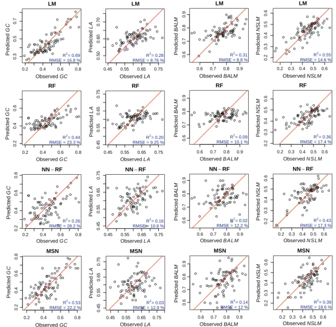
Fig. 2.Observed vs. predicted cross-validation plots for estimation methods based on the strategy of (A) direct indicator estimation (seeFig. 1). Each row correspond to an estimation method (Table 1), and columns are distributed by forest response indicator: Gini coefficient (GC), Lorenz asymmetry (LA), and proportions of basal area (BALM) and number of stems (NSLM) larger than the quadratic mean diameter. The line is the 1:1 correspondence between the values observed in the field data and the ALS-predicted values. Coefficients of determination (R2
with at least seven of the eight neighbours exceeding the height value of the centre pixel by more than five meters, were replaced with the median of the values of the neighbour pixels exceeding that threshold.
Segmentation of the CHM into individual tree crowns was based on adaptive filtering (Pitkänen et al., 2004). The CHM was first low-pass filtered using Gaussian kernels with the size of the smoothing window increasing as a function of CHM height. The segments were created around the local maxima using watershed segmenta-tion with a drainage direcsegmenta-tion following algorithm (Pitkänen, 2005). Pixels lower than two meters were masked out from the crown segments and small segments, at most three pixels in size, were combined to one of the neighbour segments based on the smallest average gradient on the segment boundary between two segments. The method and the applied parameters are described
in more detail byPackalén et al. (2013). This single-tree detection
algorithm produced altogether 3228 segments when applied to all plots of the study area. The total number of trees measured in the field was 5747, so that the success rate of the algorithm was about 56% on average. Altogether 58% of the segments contained exactly one tree, 39% more than one tree, and 3% were empty. The reader
may refer toVauhkonen et al. (2014)for more details on the
out-come obtained by this tree detection method.
The linkage between the resulting ITD segments and the field information was carried out using MSN imputation, as detailed in Vauhkonen et al. (2014). The imputations of both the ITD and S-ITD methods were based on the same segmented data, but the type of the response variable varied. Response variables in the ITD were
y= (spi,dbhi,hi,
v
i) of the largest treeiper segment. In the S-ITD,spe-cies-specific sums of volumes within each segment were used as response variables. The imputations were also carried out in a
LOO-CV fashion, i.e. the segments belonging to the same plotjas the
tar-get segment were not available as nearest neighbours, and neither they were involved in the distance metric computation. For all methods involved in strategy C, the resulting estimated tree lists
^
yC¼ N^dbh¼1;N^dbh¼2;. . .;N^dbh¼50;N^dbh¼51
n o
were aggregated at plot
level into final indicator estimates y^¼GCc;LAc;BALMd ;NSLMd ,
which were the final results compared against those in strategies A and B.
3. Results
3.1. (A) Direct indicator estimation
The first estimation strategy attempted to predict each of the
target indicators (yA) directly as univariate response (A; see
Fig. 1). Plot level LOOCV results for the resulting LM regression
estimation, RF,k-NN imputations based on RF proximity matrix,
and MSN are shown inTable 1. A more detailed evaluation of the
predictions can also be assisted by the scatterplots inFig. 2. The
LM best subset regression models (A1) obtained the lowest RMSE
and highest R2 figures in all cases: GC [R2= 0.69;
CV(RMSE) = 16.8%], LA [R2= 0.28; CV(RMSE) = 8.6%], BALM
[R2= 0.31; CV(RMSE) = 8.8%], and NSLM [R2= 0.55;
CV(RMSE) = 14.6%]. Moreover, all the LM models were unbiased, and they were found significant in their respective hypothesis
test-ing. The reader may refer to Appendix A for a more detailed
description on the best subset regression results.
In the methods based on recursive partitioning (A2 and A31), for all variables the mean squared error stabilized approximately after permuting 200–300 trees, and therefore the fixed number of 500 for the random forest was sufficient. In RF (A2), coefficients
of determination were larger for GC (R2= 0.44) and NSLM
(R2= 0.37), than forLA(R2= 0.18) andBALM(R2= 0.10). As a
conse-quence, the latter indicators showed unsatisfactory observed vs. predicted plots for RF (Fig. 2). This contingency was solved when
the RF proximity matrix was used fork-NN imputation in NN–RF
(A31), which clearly partitioned the residual variability more evenly along the full range. RF-NN was therefore more reliable than RF despite of obtaining higher RMSEs.
Comparing the two distance metrics considered for the nearest neighbour methods (A31 and A32), there was not a clear prefer-ence as results varied for each type of response. More accurate
pre-dictions were obtained with MSN (A32) forGC[CV(RMSE) = 22.2%],
while NN–RF (A31) was preferred in the case of LA
[CV(RMSE) = 10.9%], for instance. In accordance with results obtained with other methods, coefficients of determination were
higher in the cases ofGCandNSLM, thanLAandBALM. In most
cases, methods based onk-NN imputation showed a more even
distribution of residuals along the range of estimation (Fig. 2).
3.2. (B) Lorenz curve estimation
The second estimation strategy consisted in predicting discrete
quantiles of the Lorenz curve (yB) as a multivariate response with
methods based in nearest neighbour imputation (B; seeFig. 1).
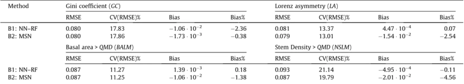
Table 2shows the comparison between the indicators obtained with the field data and those derived from the Lorenz curves estimated by imputation from the rest of plots. In this case, none of the distance metrics was demonstrated clearly superior to the other. The improvement obtained in estimating the whole Lorenz curve (B1
and B2) affected each indicator differently. In the case ofGC, better
results were obtained both for NN–RF [R2= 0.75; CV(RMSE) = 15.2%]
and MSN [R2= 0.65; CV(RMSE) = 17.9%], compared to A31 and A32.
In contrast, results forLAby NN–RF [R2= 0.06; CV(RMSE) = 12.1%]
and MSN [R2< 0.01; CV(RMSE) = 13%] were worse than those
obtained by direct estimation. Observed vs. predicted plots were also obtained in a LOOCV fashion. Both methods showed a tendency
to overestimate plots with lowBALM (Fig. 3), which effectively
signaled that most uncertainty in the prediction was in the quantiles
with higher variabilityM(.05.30). This occurred in MSN (B2) as
well, despite of z-standardizing the response.
3.3. (C) Tree list estimation
The last estimation strategy consisted in predicting the
frequen-cies at the full range ofdbhclasses, therefore producing a complete
tree list from which the Lorenz curve was afterwards generated, as
if it was the field data itself (C; seeFig. 1). Results obtained for each
Lorenz indicator derived at plot level from the resulting tree lists
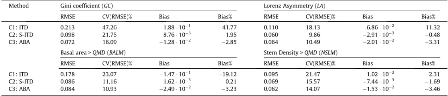
are shown in Table 3and Fig. 4. The ITD method (C1) notably
underestimated GC (41.7%) and overestimated QMD (24.87%).
This bias in determiningQMDaffectedBALMmore severely than
NSLM(Table 3), but the overall underestimation in their averaged
LAdemonstrated the ITD method unreliable for predicting the
tar-get indicators of forest structure. As it was expected, involving the understory in the semi-ITD approach (C2) improved the results
obtained by ITD. Using S-ITD, RMSEs forGC,LA,BALMandNSLM
decreased 54%, 45%, 52% and 28% respectively, compared to ITD. The best advantage was nonetheless to obtain unbiased estimates,
hence correcting the ITD underestimations observed forGCandLA.
In any case, the best results were achieved by ABA, which imputed tree lists directly at the plot level using MSN (C3). ABA for tree list imputation at plot level by MSN also obtained some of the lowest
RMSE and highestR2figures:GC[R2= 0.74; CV(RMSE) = 16.1%],LA
[R2= 0.15; CV(RMSE) = 10.5%],BALM[R2= 0.27; CV(RMSE) = 10.9%],
andNSLM[R2= 0.60; CV(RMSE) = 14.1%]. Generally speaking, the
4. Discussion
4.1. Comparing among indicators
A comparison among indicators in terms of the RMSE figures obtained can only be carried out after reflecting on the limits in the dynamic ranges that their values can obtain in real forests
(see Section2.2). The easiest way is to keep in mind the empirical
standard deviations observed in the training dataset, which were
0.137 forGC, 0.063 forLA, 0.082 forBALM, and 0.097 forNSLM.
Any comparison by RMSE and bias must account for this difference,
as the larger practical range of values forGCmakes this indicator
more prone to relative errors than e.g.LA. On the other hand, this
property also makesGCmore likely to obtain higher coefficients
of determinationR2. Considering, for instance, thatBALMandNSLM
present similar empirical variability, the former was notably more feasible to be determined by ALS remote sensing. A reason explain-ing this effect may be the fact that ALS metrics often have more explanatory power for forest variables dependent on basal area than those related to stem density (Næsset, 2002; Lefsky et al., 2005). Overall, obtaining reliable estimations was demonstrably possible for all the indicators considered, and therefore selecting the appropriate indicator of forest structure depends more on the
purpose and target forest properties than for their relation to ALS metrics.
4.2. Comparing among statistical methods
All the statistical methods considered obtained statistically sound results in terms of their RMSEs and, therefore, a number of other reasons for choosing either one may be pointed out. High-est accuracy figures in the prediction were obtained by LM regres-sion (A1), which was not surprising as this method minimized squared residuals directly for each the target indicator. However,
it can be observed inFig. 2that the residual variance followed a
pattern of underestimating high values ofGCandLA, and
overesti-mating low ones. On the other hand, the residual variance was more evenly distributed along the dynamic range of each indicator
when methods based on directk-NN imputation, which may
there-fore be preferred in such case.
RF did not seem to render special advantages for direct
indica-tor estimation, except in the case of LA, for which accuracies
obtained in A2 were comparable to those for LM (A1). The reason
for this may be the complexity of theLA indicator, asValbuena
et al. (2013b)found its separate components – namelyBALMand
NSLM– to have relations with several ALS metrics of opposite signs
NN−RF
Observed GC
Predicted
GC
R2= 0.63 RMSE = 18.7 %
NN−RF
Observed BALM
Predicted
BALM
R2= 0.18 RMSE = 10.4 %
NN−RF
Observed NSLM
Predicted
NSLM
R2= 0.36 RMSE = 20.2 %
NN−RF
Observed LA
Predicted
LA
R2= 0.08 RMSE = 12.1 %
MSN
Observed GC
Predicted
GC
R2= 0.65 RMSE = 17.9 %
MSN
Observed BALM
Predicted
BALM
R2= 0.11 RMSE = 11.3 %
MSN
Observed NSLM
Predicted
NSLM
R2= 0.31 RMSE = 19.8 %
0.2 0.4 0.6 0.8 0.45 0.55 0.65 0.75 0.6 0.7 0.8 0.9 0.2 0.3 0.4 0.5 0.6
0.2 0.4 0.6 0.8 0.45 0.55 0.65 0.75 0.6 0.7 0.8 0.9 0.2 0.3 0.4 0.5 0.6
0.2
0.4
0.6
0.8
0.6
0.7
0.8
0.9
0.2
0.3
0.4
0.5
0.6
0.50
0.60
0.70
0.2
0.4
0.6
0.6
0.7
0.8
0.9
0.2
0.3
0.4
0.5
0.6
0.45
0.55
0.65
0.75
MSN
Observed LA
Predicted
LA
R2= 0.00 RMSE = 13 %
Fig. 3.Observed vs. predicted cross-validation plots for estimation methods based on the strategy of (B) Lorenz curve estimation (seeFig. 1). Each row correspond to an estimation method (Table 2), and columns are distributed by forest response indicator: Gini coefficient (GC), Lorenz asymmetry (LA), and proportions of basal area (BALM) and number of stems (NSLM) larger than the quadratic mean diameter. The line is the 1:1 correspondence between the values observed in the field data and the ALS-predicted values. Coefficients of determination (R2
) and coefficients of variation of the RMSE (denoted as RMSE) are listed for each plot.Table 2summarizes the RMSEs that correspond to each of these plots.
Table 2
Accuracy assessment results for estimation methods based on the strategy of (B) Lorenz curve estimation (seeFig. 1). NN–RF: nearest neighbour based on random forest (B1); MSN: most similar neighbour (B2).
Method Gini coefficient (GC) Lorenz asymmetry (LA)
RMSE CV(RMSE)% Bias Bias% RMSE CV(RMSE)% Bias Bias%
B1: NN–RF 0.080 17.83 1.06102
2.36 0.081 13.37 4.47104
0.07
B2: MSN 0.080 17.86 1.73103
0.38 0.079 13.01 1.54102
2.54
Basal area >QMD(BALM) Stem Density >QMD(NSLM)
RMSE CV(RMSE)% Bias Bias% RMSE CV(RMSE)% Bias Bias%
B1: NN–RF 0.087 11.27 1.39103
0.18 0.093 21.14 4.95104
0.11
B2: MSN 0.087 11.25 1.06102
1.38 0.087 19.79 2.01102
(either direct or indirect). In such type of cases, recursive partition-ing may allow to express the relations of ALS metrics against each of those components, explaining different portions of variance sep-arately at different branches of a regression tree (Hastie et al., 2009). This may also explain why direct estimation of LA was one of the few cases in which NN–RF estimation was more accurate than MSN. Otherwise, the generality was for MSN to outperform
NN–RF. This result differs from those obtained by Hudak et al.
(2008) for other type of forest variables. On the other hand, Packalén et al. (2012)found NN–RF to perform better than MSN
for univariate responses, while the latter was more beneficial in the multivariate case.
4.3. Comparing among estimation strategies
In principle, direct indicator estimation (strategy A) can be, by definition, expected to obtain the lowest RMSE figures across all methodologies compared. However, tree list estimation by MSN from ALS metrics obtained at plot level was demonstrably beneficial with regards to estimating some of the indicators of for-0.2 0.4 0.6 0.8
0.1
0.3
0.5
ITD
Observed G C
Predicted
GC
R2= 0.51 RMSE = 47.3 %
0.45 0.55 0.65 0.75
0.40
0.50
0.60
0.70
ITD
Observed L A
Predicted
LA
R2= 0.01 RMSE = 18.1 %
0.5 0.7 0.9
0.4
0.6
0.8
ITD
Observed B A L M
Predicted
BALM
R2= 0.16 RMSE = 23.1 %
0.2 0.3 0.4 0.5 0.6
0.3
0.4
0.5
0.6
ITD
Observed N S L M
Predicted
NSLM
R2= 0.11 RMSE = 21.5 %
0.2 0.4 0.6 0.8
0.2
0.4
0.6
S−ITD
Observed G C
Predicted
GC
R2= 0.52 RMSE = 21.8 %
0.45 0.55 0.65 0.75
0.45
0.55
0.65
0.75
S−ITD
Observed L A
Predicted
LA
R2= 0.20 RMSE = 9.86 %
0.6 0.7 0.8 0.9
0.5
0.6
0.7
0.8
0.9
S−ITD
Observed B A L M
Predicted
BALM
R2= 0.13 RMSE = 11.2 %
0.2 0.3 0.4 0.5 0.6
0.2
0.3
0.4
0.5
0.6
S−ITD
Observed N S L M
Predicted
NSLM
R2= 0.49 RMSE = 15.6 %
0.2 0.4 0.6 0.8
0.2
0.4
0.6
ABA
Observed G C
Predicted
GC
R2= 0.74 RMSE = 16.1 %
0.45 0.55 0.65 0.75
0.45
0.55
0.65
0.75
ABA
Observed L A
Predicted
LA
R2= 0.15 RMSE = 10.5 %
0.6 0.7 0.8 0.9
0.6
0.7
0.8
0.9
ABA
Observed B A L M
Predicted
BALM
R2= 0.27 RMSE = 10.9 %
0.2 0.3 0.4 0.5 0.6
0.2
0.3
0.4
0.5
0.6
ABA
Observed N S L M
Predicted
NSLM
R2= 0.60 RMSE = 14.1 %
Fig. 4.Observed vs. predicted cross-validation plots for estimation methods based on the strategy of (C) tree list estimation (seeFig. 1). Each row correspond to an estimation method (Table 3), and columns are distributed by forest response indicator: Gini coefficient (GC), Lorenz asymmetry (LA), and proportions of basal area (BALM) and number of stems (NSLM) larger than the quadratic mean diameter. The line is the 1:1 correspondence between the values observed in the field data and the ALS-predicted values. Coefficients of determination (R2
) and coefficients of variation of the RMSE (denoted as RMSE) are listed for each plot.Table 3summarizes the RMSEs that correspond to each of these plots.
Table 3
Accuracy assessment results for estimation methods based on the strategy of (C) tree list estimation (seeFig. 1). ITD: individual tree detection (C1); S-ITD: semi-ITD (C2); ABA: MSN tree list estimation at plot level (C3).
Method Gini coefficient (GC) Lorenz Asymmetry (LA)
RMSE CV(RMSE)% Bias Bias% RMSE CV(RMSE)% Bias Bias%
C1: ITD 0.213 47.26 1.88101
41.77 0.110 18.13 6.86102
11.32
C2: S-ITD 0.098 21.75 8.76103 1.95 0.060 9.86
2.91103
0.48
C3: ABA 0.072 16.09 1.28102
2.85 0.064 10.49 2.01102
3.31
Basal area >QMD(BALM) Stem Density >QMD(NSLM)
RMSE CV(RMSE)% Bias Bias% RMSE CV(RMSE)% Bias Bias%
C1: ITD 0.178 23.07 1.47101
19.12 0.095 21.47 1.02102
2.31
C2: S-ITD 0.086 11.16 1.62103
0.21 0.069 15.57 7.44103
1.69
C3: ABA 0.084 10.93 2.49102
3.23 0.062 14.07 1.53102
est structure considered in this study. This can happen if the appli-cation of a given study benefits from having detailed information on the entire diameter distribution (Gobakken and Næsset, 2004; Maltamo et al., 2007). This seems to be the case for the structural indicators selected. Additionally, many stand attributes, such as basal area, number of stems, volume, or timber assortments and their value (Vauhkonen et al., 2014), can be flexibly calculated from the same tree list model which is constructed for the purpose of forest structure characterization. When comparing the MSN estimation, which was common for all strategies, RMSE results obtained in tree list estimation (C3) improved those obtained by Lorenz curve estimation (B2) and direct indicator estimation (A32), generally speaking. Consequently, the results presented in this article may reveal that approaches for tree list estimation (strategy C) could as well be advantageous in describing tree size inequality and the balance between understory and overstory.
The strategy of estimating the whole Lorenz curve (B;Fig. 1)
obtained accuracies in between the other two. No benefit was observed in comparison to estimating its corresponding diameter distribution, and therefore strategy C is preferred. One reason can be an accumulation of methodological errors, for instance when splitting the continuous Lorenz curve into discrete quantiles, or while retrieving the curve’s inflexion point. Further research could consider using narrower bin sizes, or predicting basal
area-weighted and unweighted distributions simultaneously
(Gobakken and Næsset, 2004; Maltamo et al., 2007), in pursue of the final Lorenz curve. In light of these results, there is no interest in estimating the full Lorenz curve when pursuing a prediction of target indicators. There may, however, still be interest in studying
the canonical components themselves (e.g.Lefsky et al., 2005), as
they can provide with information on the importance of different ALS metrics at diverse portions of the Lorenz curve, therefore relat-ing them to relations among vertical strata (Valbuena et al., 2014).
4.4. Individual tree detection vs. area-based estimation
The adaptive filtering used for ITD was devoted to detecting the presence of small trees as well as large ones, as the amplitude of the filter was roughly proportional to crown size at different tree layers (Pitkänen et al., 2004). In spite of this, the results obtained
with ITD were negatively biased forGC(Table 3). Thus, understory
ingrowth below the dominant canopy remained undetected, and hence tree size inequality was clearly underestimated. The
under-estimation inLAalso revealed that understory trees are more likely
missed when they are smaller (Valbuena et al., 2013a). When the interpretation is based on 2.5-dimensional CHMs, small trees are inherently missed when overtopped by larger ones (Vauhkonen et al., 2012). AlthoughVauhkonen et al. (2014)showed that this affected only to 13% of the total stem volume, the effect on forest structure indicators is clearly higher. The relatively low rate of suc-cess in tree detection for the specific the method employed, and the fact that failure in tree detection happened with higher proba-bility on suppressed trees than dominant ones, led to underesti-mated tree size inequality. Thus the success achieved by semi-ITD, which improved the ITD results by simply accounting for all the trees enclosed within a segment, is logical and expected. Our results, however, do not preclude other ITD methods with higher tree detection rates of success to obtain better estimations of forest structure indicators. Further research could therefore consider other ITD techniques, such as those based on point segmentation (Li et al., 2012).
Plot level imputation of tree lists following the ABA method obtained the lowest RMSEs for most indicators among all the tree list methods tested (Table 3). This may indicate that segmenting and interpreting a 2.5-dimensional CHM burdens the evaluation of structural properties from forests. However, this was not the
case for LA, a result we found most intriguing. Also Vastaranta
et al. (2012)found that the preference for either ABA or ITD may depend on the target forest response. The reason may be grounded
on the fact that LA is an indicator on the relative relationships
between over and understory both in terms of stem density and basal area (Valbuena et al., 2013b). Consequently, although semi-ITD seemed insufficiently reliable for determining tree size
inequality (GC), it can provide a reasonable idea on the relations
of dominance among individual trees in multilayered forests. How-ever, we found that computing ALS metrics at the plot level to be more informative than using CHM segments, in terms of the indi-cators chosen. We therefore recommend the use of ABA above ITD when analyzing structural properties of complex diameter distri-butions, unless the purpose of a given study requires the detail given at tree crown scale, e.g. research on individual tree competition.
4.5. Effect of scale in estimation of Lorenz-based indicators
The effect of scale on the Lorenz indicators considered was one
important issue already mentioned inValbuena et al. (2013a). As
this study was carried out using plots differing in size, there could be a potential small influence of the scale on the results. However, as plot size was determined according to stand density, the num-ber of trees included at each of them can be considered roughly similar. Therefore, even though the 79 cases used for these estima-tions differ in plot area, they are equal in terms of sample size. Moreover, the scale used also affects different ALS metrics in a dis-similar way, and it is not clear whether these effects are synergetic for the Lorenz indicators and the ALS metrics, affecting the estima-tion itself. In any case, for the purpose of this study we have con-sidered it to be small effect affecting equally across all the methods and strategies considered. Whether these indicators are more affected by the scale or the sample size, or this effect is also affecting the ALS estimation of Lorenz indicators, are questions to be clarified in future research.
5. Conclusions
Results were statistically sound for all the methods based on ABA, and therefore the choice of method may depend more on the properties of the outcoming estimates, such as the distribution of the residual variance. When MSN imputation was used to com-pute an entire diameter distribution, the accuracy of the resulting indicators was higher than when estimating the Lorenz curve or approaching those same indicators directly. Therefore, tree list estimation can be of interest in studies focused on the structural properties of forests. Lorenz curve estimation may be
advanta-Table A1
Description of metrics computed from ALS return heights (seeMcGaughey, 2012).
Predictor Description
P05 5th percentile P70 70th percentile
L.CV coefficient of variation (ratio between second and first L-moments)
L4 Fourth L-moment
MAD.median Median absolute deviation from the median Skew Third product moment (skewness)
Cover Percentage of all returns above a height threshold of 1 m Cover.mode Percentage of all returns above their mode
Cover.f.mode Percentage of first returns above their mode Cover.mean/
f
Ratio between the percentage of all returns above their mean and the total number of first returns, in percentage Cover.mode/
f
geous if interested in a deeper exploration on the relations of dom-inance among canopy strata, but not for indicator estimation. Finally, although the semi-ITD approach may correct the biasing underestimation of tree size inequality obtained by ITD, any approach involving CHM segmentation was demonstrably inferior to plot level training, with regards to estimating forest structure indicators based on the Lorenz curve.
Acknowledgments
Rubén Valbuena’s work was funded by Metsähallitus Grant and the Foundation for European Forest Research (FEFR). This study was also partly funded by the strategic funding of the University of Eastern Finland.
Appendix A. Detail on results for best subset selection models (LM)
In regression modelling, the selection of independent variables was carried out by imposing a maximum number of five predictors and the criterion of lowest AICc. The resulting models obtained
AICc values of 181.32,238.36,198.85 and 206.18
respec-tively forGC,LA,BALMandNSLM. It is worth noting that this
crite-ria yielded best subset models with five predictors, except in the
case ofLAwhich included only three. These final models were:
GC¼b0þb1L:CVþb2P05þb3Co
v
erþb4Co
v
er:modeþb5Cov
er:f:mode ðA:1ÞLA¼b0þb1L4þb2MAD:medianþb3Co
v
er:mode=f ðA:2ÞBALM¼b0þb1L4þb2MAD:medianþb3Skewþb4
Co
v
erþb5Cov
er:f:mode ðA:3ÞNSLM¼b0þb1P70þb2Co
v
erþb3Cov
er:modeþb4Co
v
er:mean=fþb5Cov
er:mode=f ðA:4ÞTable A1includes a legend explaining these predictors, whereas Table A2lists the regression estimates and results of hypothesis testing.
References
Andersen, H., McGaughey, R.J., Reutebuch, S.E., 2005. Estimating forest canopy fuel parameters using LIDAR data. Remote Sens. Environ. 94 (4), 441–449. Axelsson, P.(, 2000. DEM Generation from laser scanner data using adaptive TIN
models. Int. Arch. Photogramm. Remote Sens. 33 (Part B4), 110–117. Bollandsås, O.M., Næsset, E., 2007. Estimating percentile-based diameter
distributions in uneven-sized Norway spruce stands using airborne laser scanner data. Scand. J. For. Res. 22 (1), 33–47.
Breidenbach, J., Næsset, E., Lien, V., Gobakken, T., Solberg, S., 2010. Prediction of species specific forest inventory attributes using a nonparametric semi-individual tree crown approach based on fused airborne laser scanning and multispectral data. Remote Sens. Environ. 114 (4), 911–924.
Burger, J.A., 2009. Management effects on growth, production and sustainability of managed forest ecosystems: past trends and future directions. Forest Ecol. Manage. 258 (10), 2335–2346.
Crookston, N.L., Finley, A.O., 2008. YaImpute: an R package forjNN imputation. J. Stat. Softw. 23 (10), 1–16.
Damgaard, C., Weiner, J., 2000. Describing inequality in plant size or fecundity. Ecology 81 (4), 1139–1142.
Duduman, G., 2011. A forest management planning tool to create highly diverse uneven-aged stands. Forestry 84 (3), 301–314.
Eskelson, B.N.I., Temesgen, H., Lemay, V., Barrett, T.M., Crookston, N.L., Hudak, A.T., 2009. The roles of nearest neighbor methods in imputing missing data in forest inventory and monitoring databases. Scand. J. For. Res. 24 (3), 235–246. Falkowski, M.J., Evans, J.S., Martinuzzi, S., Gessler, P.E., Hudak, A.T., 2009.
Characterizing forest succession with lidar data: an evaluation for the Inland Northwest, USA. Remote Sens. Environ. 113 (5), 946–956.
Gobakken, T., Næsset, E., 2004. Estimation of diameter and basal area distributions in coniferous forest by means of airborne laser scanner data. Scand. J. Forest Res. 19 (6), 529–542.
Gove, J.H., 2004. Structural stocking guides: a new look at an old friend. Can. J. Forest Res. 34 (5), 1044–1056.
Gove, J.H., Patil, G.P., 1998. Modeling the basal area-size distribution of forest stands: a compatible approach. Forest Sci. 44 (2), 285–297.
Hall, S.A., Burke, I.C., Box, D.O., Kaufmann, M.R., Stoker, J.M., 2005. Estimating stand structure using discrete-return lidar: an example from low density, fire prone ponderosa pine forests. Forest Ecol. Manage. 208 (1–3), 189–209.
Hastie, T., Tibshirani, R., Friedman, J.H., 2009. The Elements of Statistical Learning. Data Mining, Inference, and Prediction. Springer, New York.
Hill, R.A., Broughton, R.K., 2009. Mapping the understorey of deciduous woodland from leaf-on and leaf-off airborne LiDAR data: a case study in lowland Britain. ISPRS J. Photogramm. Remote Sens. 64 (2), 223–233.
Table A2
Summary of results for regression estimates and their hypothesis testing.
Regression coefficient Gini coefficient (GC) Lorenz asymmetry (LA)
Estimate SE t-Student p-value Estimate SE t-Student p-value
b0 3.10 0.39 7.89 <0.001*** 0.71 6.61102 10.77 <0.001***
b1 5.44 0.45 11.95 <0.001*** 0.20 3.20102 6.52 <0.001***
b2 2.32 0.73 3.16 0.002** 7.88103 2.89103 2.73 0.008**
b3 3.91102 3.00103 13.08 <0.001*** 9.61104 4.80104 2.00 0.048*
b4 5.90102 9.08103 6.50 <0.001***
b5 4.16102 9.21103 4.51 <0.001***
R2adj. RSE F-Fisher p-value R2adj. RSE F-Fisher p-value
0.72 7.24102 41.47 <0.001*** 0.34 5.13
102 14.39 <0.001***
Basal area >QMD(BALM) Stem density >QMD(NSLM)
Estimate SE t-Student p-value Estimate SE t-Student p-value
b0 1.14 0.25 4.61 <0.001*** 0.32 0.19 1.72 0.089
b1 0.38 6.95102 5.41 <0.001*** 7.11103 2.73103 2.61 0.011*
b2 1.75102 5.15103 3.39 <0.001*** 1.19102 1.24103 9.62 <0.001***
b3 0.29 4.74102 6.17 <0.001*** 1.17102 2.30103 3.92 <0.001***
b4 1.19102 2.03103 5.56 <0.001*** 1.10102 1.63103 6.74 <0.001***
b5 1.16102 3.34103 3.48 <0.001*** 8.21103 1.28103 6.42 <0.001***
R2
adj. RSE F-Fisher p-value R2
adj. RSE F-Fisher p-value
0.37 6.48102 10.44 <0.001*** 0.59 5.13
102 23.70 <0.001***
SE: standard error. RME: residual standard error.R2
adj.: coefficient of determination adjusted by degrees of freedom. Levels of significance: NS = not significant (p-value > 0.05).
<0.01.
*<0.05.
** <0.01. ***
Hosking, J.R.M., 1990. L-Moments: analysis and estimation of distributions using linear combinations of order statistics. J. R. Stat. Soc. Ser. B (Methodological) 52 (1), 105–124.
Hudak, A.T., Crookston, N.L., Evans, J.S., Hall, D.E., Falkowski, M.J., 2008. Nearest neighbor imputation of species-level, plot-scale forest structure attributes from LiDAR data. Remote Sens. Environ. 112 (5), 2232–2245.
Knox, R.G., Peet, R.K., Christensen, N.L., 1989. Population dynamics in loblolly pine stands: changes in skewness and size inequality. Ecology 70 (4), 1153–1167. Korpela, I., Tuomola, T., Välimäki, E., 2007. Mapping forest plots: an efficient method
combining photogrammetry and field triangulation. Silva Fenn. 41 (3), 457– 469.
Lähivaara, T., Seppänen, A., Kaipio, J.P., Vauhkonen, J., Korhonen, L., Tokola, T., Maltamo, M., 2013. Bayesian approach to tree detection based on airborne laser scanning data. IEEE Trans. Geosci. Remote Sens. 52 (5), 2690–2699.
Lefsky, M.A., Cohen, W.B., Parker, G.G., Harding, D.J., 2002. Lidar remote sensing for ecosystem studies. Bioscience 52 (1), 19–30.
Lefsky, M.A., Hudak, A.T., Cohen, W.B., Acker, S.A., 2005. Patterns of covariance between forest stand and canopy structure in the Pacific Northwest. Remote Sens. Environ. 95 (4), 517–531.
Lexerød, N.L., Eid, T., 2006. An evaluation of different diameter diversity indices based on criteria related to forest management planning. Forest Ecol. Manage. 222 (1), 17–28.
Li, W., Guo, Q., Jakubowski, M., Kelly, M., 2012. A new method for segmenting individual trees from the lidar point cloud. Photogramm. Eng. Remote Sens. 78, 75–84.
Liaw, A., Wiener, M., 2002. Classification and regression by randomForest. R News 2 (3), 18–22.
Lindberg, E., Holmgren, J., Olofsson, K., Wallerman, J., Olsson, H., 2010. Estimation of tree lists from airborne laser scanning by combining single-tree and area-based methods. Int. J. Remote Sens. 31 (5), 1175–1192.
Magnussen, S., Boudewyn, P., 1998. Derivations of stand heights from airborne laser scanner data with canopy-based quantile estimators. Can. J. Forest Res. 28 (7), 1016–1031.
Maltamo, M., Packalen, P., 2014. Species specific management inventory in Finland. In: Maltamo, M., Naesset, E., Vauhkonen, J. (Eds.),Forestry Applications of Airborne Laser scanning: Concepts and Case Studies. Managing Forest Ecosystems, vol. 27. Springer, Dordrecht.
Maltamo, M., Eerikäinen, K., Pitkänen, J., Hyyppä, J., Vehmas, M., 2004. Estimation of timber volume and stem density based on scanning laser altimetry and expected tree size distribution functions. Remote Sens. Environ. 90 (3), 319– 330.
Maltamo, M., Packalén, P., Yu, X., Eerikäinen, K., Hyyppä, J., Pitkänen, J., 2005. Identifying and quantifying structural characteristics of heterogeneous boreal forests using laser scanner data. Forest Ecol. Manage. 216 (1), 41–50. Maltamo, M., Malinen, J., Packalén, P., Suvanto, A., Kangas, J., 2006. Nonparametric
estimation of stem volume using airborne laser scanning, aerial photography, and stand-register data. Can. J. Forest Res. 36 (2), 426–436.
Maltamo, M., Suvanto, A., Packalén, P., 2007. Comparison of basal area and stem frequency diameter distribution modelling using airborne laser scanner data and calibration estimation. Forest Ecol. Manage. 247 (1–3), 26–34.
Maltamo, M., Næsset, E., Bollandsås, O.M., Gobakken, T., Packalén, P., 2009. Non-parametric prediction of diameter distributions using airborne laser scanner data. Scand. J. Forest Res. 24 (6), 541–553.
Martinuzzi, S., Vierling, L.A., Gould, W.A., Falkowski, M.J., Evans, J.S., Hudak, A.T., et al., 2009. Mapping snags and understory shrubs for a LiDAR-based assessment of wildlife habitat suitability. Remote Sens. Environ. 113 (12), 2533–2546.
McGaughey, R.J., 2012. FUSION/LDV: Software for LIDAR Data Analysis and Visualization. Version 3.10. Pacific Northwest Research Station. USDA Forest Service, Seattle, WA.
McInerney, D.O., Suarez-Minguez, J., Valbuena, R., Nieuwenhuis, M., 2010. Forest canopy height retrieval using LiDAR data, medium-resolution satellite imagery and kNN estimation in Aberfoyle, Scotland. Forestry 83 (2), 195–206. Moeur, M., Stage, A.R., 1995. Most similar neighbor: an improved sampling
inference procedure for natural resource planning. Forest Sci. 41 (2), 337–359.
Næsset, E., 2002. Predicting forest stand characteristics with airborne scanning laser using a practical two-stage procedure and field data. Remote Sens. Environ. 80 (1), 88–99.
Ozdemir, I., Donoghue, D.N.M., 2013. Modelling tree size diversity from airborne laser scanning using canopy height models with image texture measures. Forest Ecol. Manage. 295 (1), 28–37.
Packalén, P., Maltamo, M., 2008. Estimation of species-specific diameter distributions using airborne laser scanning and aerial photographs. Can. J. Forest Res. 38 (7), 1750–1760.
Packalén, P., Temesgen, H., Maltamo, M., 2012. Variable selection strategies for nearest neighbor imputation methods used in remote sensing based forest inventory. Can. J. Remote Sens. 38 (5), 557–569.
Packalén, P., Vauhkonen, J., Kallio, E., Peuhkurinen, J., Pitkänen, J., Pippuri, I., Strunk, J., Maltamo, M., 2013. Predicting the spatial pattern of trees with airborne laser scanning. Int. J. Remote Sens. 34 (14), 5154–5165.
Persson, Å., Holmgren, J., Söderman, U., 2002. Detecting and measuring individual trees using an airborne laser scanner. Photogramm. Eng. Remote Sens. 68 (9), 925–932.
Pitkänen, J., 2005. A multi-scale method for segmentation of trees in aerial images. In: Hobbelstad, K., (Ed.). In: Proceedings of the SNS-meeting at Sjusjøen – Forest Inventory and Planning in Nordic Countries. NIJOS-report 09/05, Norwegian Institute of Land Inventory, Oslo, Norway.
Pitkänen, J., Maltamo, M., Hyyppä, J., Yu, X., 2004. Adaptive methods for individual tree detection on airborne laser based canopy height model. Int. Arch. Photogramm., Remote Sens. Spatial Inform. Sci. 36 (Part 8/W2), 187–191. R Development Core Team, 2011. R: A Language and Environment for Statistical
Computing.
Reitberger, J., Schnörr, C., Krzystek, P., Stilla, U., 2009. 3D segmentation of single trees exploiting full waveform LIDAR data. ISPRS J. Photogramm. Remote Sens. 64 (6), 561–574.
Suárez, J.C., García, R., Gardiner, B.A., Patenaude, G., 2008. The estimation of wind risk in forest stands using ALS. J. Forest Plann. 13 (Silvilaser Special Issue), 165–186. Sugiura, N., 1978. Further analysts of the data by akaike’ s information criterion and
the finite corrections. Commun. Stat. – Theory Methods 7 (1), 13–26. Valbuena, R., Packalén, P., Martín-Fernández, S., Maltamo, M., 2012. Diversity and
equitability ordering profiles applied to study forest structure. Forest Ecol. Manage. 276, 185–195.
Valbuena, R., Packalén, P., Mehtätalo, L., García-Abril, A., Maltamo, M., 2013a. Characterizing forest structural types and Shelterwood dynamics from Lorenz-based indicators predicted by airborne laser scanning. Can. J. Forest Res. 43 (11), 1063–1074.
Valbuena, R., Maltamo, M., Martín-Fernández, S., Packalén, P., Pascual, C., Nabuurs, G.J., 2013b. Patterns of covariance between airborne laser scanning metrics and Lorenz curve descriptors of tree size inequality. Can. J. Remote Sens. 39 (S1), S18–S31.
Valbuena, R., Packalén, P., Tokola, T., Maltamo, M., 2014. Canonical correlation analysis for interpreting relations of airborne laser scanning metrics along the Lorenz curve of tree size inequality. Baltic Forestry 20 (2) (in press). Vastaranta, M., Kankare, V., Holopainen, M., Yu, X., Hyypä, J., Hyypä, H., 2012.
Combination of individual tree detection and area-based approach in imputation of forest variables using airborne laser data. ISPRS J. Photogramm. Remote Sens. 67 (1), 73–79.
Vauhkonen, J., Korpela, I., Maltamo, M., Tokola, T., 2010. Imputation of single-tree attributes using airborne laser scanning-based height, intensity, and alpha shape metrics. Remote Sens. Environ. 114 (6), 1263–1276.
Vauhkonen, J., Ene, L., Gupta, S., Heinzel, J., Holmgren, J., Pitkänen, J., Solberg, S., Wang, Y., Weinacker, H., Hauglin, K.M., Lien, V., Packalén, P., Gobakken, T., Koch, B., Næsset, E., Tokola, T., Maltamo, M., 2012. Comparative testing of single-tree detection algorithms under different types of forest. Forestry 85 (1), 27–40. Vauhkonen, J., Packalen, P., Malinen, J., Pitkänen, J., Maltamo, M., 2014. Airborne
laser scanning based decision support for wood procurement planning. Scand. J. Forest Res., 29 (in press).