Temperature regulation of a pilot-scale batch reaction system via explicit model predictive control

Temperature regulation of a pilot-scale batch

reaction system via explicit model predictive control

Javier Sanchez-Cossio, Juan David Ortega-Alvarez

Universidad EAFIT Medell´ın, Colombia

Email:{jsanch10, jortega}@eafit.edu.co

Carlos Ocampo-Martinez

IEEE Senior Member

Institut de Rob`otica i Inform`atica Industrial (CSIC-UPC) Universitat Polit`ecnica de Catalunya (UPC)

Barcelona, Spain Email: [email protected]

Abstract—In this paper, the temperature of a pilot-scale batch reaction system is modeled towards the design of a controller based on the explicit model predictive control (EMPC) strategy. Some mathematical models are developed from experimental data to describe the system behavior. The simplest, yet reliable, model obtained is a (1,1,1)-order ARX polynomial model for which the mentioned EMPC controller has been designed. The resultant controller has a reduced mathematical complexity and, according to the successful results obtained in simulations, will be used directly on the real control system in a next stage of the entire experimental framework.

I. INTRODUCTION

Several industrial systems within the process control frame-work are regulated via traditional control strategies, which have been worked on conveniently during last years according to particular management objectives and operation criteria. However, new strategies and methodologies to improve the performance of processes and devices have raised in order to innovate in the traditional industrial environments. To this end and having available a complete, robust and versatile pilot-scale batch reaction system, it is worthy to perform research towards the potential implementation of existing control techniques in such a way that real-time controllers may be implemented and potentially transferred to the actual implementation within real processes. The Department of Pro-cess Engineering at EAFIT University in Medell´ın (Colombia) has an equipment for studying batch processes from which the temperature loop is here considered. This loop should maintain the temperature inside the reaction vessel close to a reference value by manipulating some system devices. To accomplish this, the model-based predictive control (MPC) strategies are considered since they have had a significant impact in industrial application due to their ability to tackle complex problems, optimizing the behavior of the plant by using a dynamical model to predict its response to the control signals and thus selecting the most suitable value according to the objectives defined. Renowned chemical companies like Repsol YPF have implemented model-based predictive con-trollers to large-scale batch reactors with advantageous results, e.g., improved product quality, shorter batch duration, and higher equipment availability [1].

Different works have highlighted the limitations of tradi-tional controllers dealing with batch reaction systems: actuator delays, temperature overshoot during the heating-up stage

and significantly different dynamics between the heating and cooling stages, just to mention some of them [1], [2]. Often, these works point out to MPC controllers as the best alternative to overcome that mentioned issues. Moreover, MPC is posed as a suitable alternative to design decentralized multivariable PID controllers in applications like biodiesel reactors, where com-plex decoupling techniques are required, yet not completely effective [3]. Many of this works provide with evidence of the advantages of MPC in such systems using simulations [4], [5], [6] while some others moved to real-scale implementa-tion with success [1], although few is available on dealing with the computational requirements of such implementation in average industrial control equipment. Ho et al. [3] used centralized adaptive generalized predictive control (CA-GPC) to handle multiple control loops of a transesterification batch reactor, instead of using a decentralized multiple-controller strategy. They draw upon a validated phenomenological model of the transesterification process and used ARX models to both represent and simplify its different components. Results from simulations show that the performance of the CA-GPC controller was far more effective for temperature control than a well-tuned decentralized PID, although just comparable for the control of methyl-ester concentration. Nevertheless, the authors acknowledge the computational complexity inherent to the real implementation of such control scheme and propose the lab-scale implementation as the next step.

The work reported in this paper comprises the development and results analyses of the design of an explicit MPC controller (EMPC) for temperature control of the aforementioned pilot-scale batch reactor. The main contribution of this paper consists in making the designed EMPC controller streamlined enough to be implemented in the equipment as simple as a medium-profile PLC without losing its advantages in performance. The controller reported here has a reduced mathematical complex-ity and will be used directly on the real control system powered by an S7-300 PLC.

The remainder of this paper is organized as follows. In Section II, a short functional description of the case study is presented in order to clarify the structure of the physical system and establish some guidelines for its modeling. Then, in Sections III and IV, some autoregressive models formulated for the system are presented. From the simplest ARX model obtained, the EMPC controller is designed in Section V. Finally, some conclusions are drawn in Section VI.

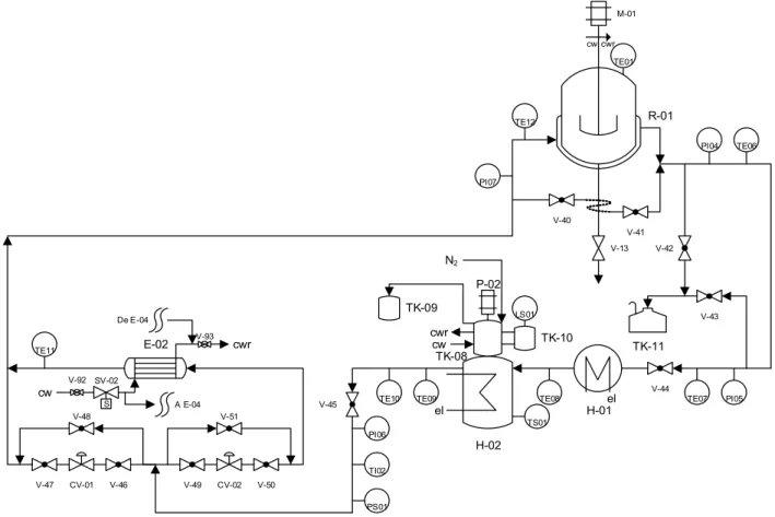
R-01

V-13 V-42 V-41

V-44

PI04 TE06

V-43

TK-11

PI05 TE07 LS01

H-02 el

TK-08

TK-10 TK-09

cw cwr N2

TE08 TE09

TE10

PI06

TI02

PS01 V-45

CV-02 V-51

V-49 V-50 CV-01

V-48

V-47 V-46

E-02

cw

cwr

V-40

S SV-02 TE11

PI07 TE12

V-93

V-92

H-01el

De E-04

A E-04

TS01

TE01 cw cwr

P-02

M-01

Figure 1. Process flow diagram of the case study

II. SYSTEMDESCRIPTION

The temperature control equipment studied consists of a thermal fluid circuit that supplies the required thermal energy to the reaction vessel or removes surplus heat according to the process needs. The final goal is to maintain the temper-ature inside the reaction vessel close to a reference value by manipulating some system devices (actuators). A process flow diagram (PFD) for this system is presented in Figure 1.

The thermal fluid is heated by a couple of electrical coil heaters (H-01, H-02) and pumped by P-02. The fluid then flows through pipeline towards the jacketed reaction vessel and back to the heaters. Along the way, there are several elements, such as valves and temperature/pressure sensors, which allow the measurement of some variables and the manipulation of the flow. After passing through the heaters, the fluid goes to the jacket through one of two paths: the former delivers it directly while the latter passes through a heat exchanger where the fluid can be cooled down if needed by means of cooling water. Thus, the action of heating the fluid is accomplished by turning on the electrical coils inside the heaters and cooling is reached by enabling the flow through the cooling water heat exchanger (E-02).

The temperature of the thermal fluid after the electric coil heaters is measured by the sensor TE-10 and, before entering the vessel’s jacket, it is measured by TE-12. Sensor TE-06 is located at the jacket output, while TE-07 is placed before the heaters inlet. The controlled variable is the temperature of the

reacting mixture inside the vessel, measured using the sensor TE-01. The manipulated variables are heating and cooling actions of the thermal fluid, accomplished as described.

This equipment uses a SIEMENS S7-300 PLC for the monitoring and control of sensors and actuators and has a touchscreen panel for operator interaction. The data from temperature sensors is stored every minute, a value that is used as the sampling time for the controllers given that this is a relatively slow process and this time value yields in a suitable tracking of the process temperature behavior.

III. ARX MODELING

ARX models are linear difference equations of the form

A(q)y(t) =B(q)u(t) +e(t), (1) where A(q) and B(q) are polynomials in the delay operator

(q−1_{) of order according to the desired order for the model}

(na, nb, nk).nais the order of the polynomialA(q)andnbis the order of the polynomial B(q). These determine the order of the delay operator in each case.nkis the input-output delay. This structure implies that the current output is predicted as a weighted sum of past output values and current and past input values [7],[8].

To describe the case study of this paper by using ARX models, a set of control volumes1 was defined and, for each one, an ARX model was calculated. The corresponding coef-ficients were obtained from a set of experimental data using

System Identification Toolbox in MATLAB [8]. A suitable set of models for the considered variables was produced. The control volumes are defined as follows (according to Figure 1):

• The reaction vessel, where the reaction mixture is contained and the reaction takes place. Its temperature,

T01, is influenced by the transfer from the thermal

fluid and the loss to the environment. There can also be some reaction heat but, since this is a preliminary work, it is neglected here. This control volume will be referred to with the subscriptR.

• The reaction vessel jacket, where the transfer between the thermal fluid and the reaction mixture takes place to either supply or remove the required energy. This control volume will be referred to with the subscript

j and its boundaries are devices TE-12 and TE-06. • The piping and equipment between the output of the

vessel jacket and the output of the fluid heater H-02. This control volume is bound by devices TE-06 and TE-10 and will be referred to asp1. Here, the thermal

fluid is heated by using electrical coils and some loss to the environment also occurs.

• The piping and equipment between the output of the fluid heater H-02 and the inlet to the vessel jacket. This control volume is referred to asp2 and is bound

by TE-10 and TE-12. The thermal fluid cooler E-02, which removes energy from the thermal fluid when it is needed to cool down the vessel, is placed here. Some loss to the environment also occurs.

The measured temperatures are, accordingly,T01,T06,T10

andT12, beingT01the output whose behavior is controlled. As

said, the manipulated inputs are the heating and cooling actions of the thermal fluid. Heating is accomplished by turning on the electric heaters. These heaters have a fixed power and thus, for modeling purposes, a variable H can be assigned to represent heating and the regression from experimental datasets will give suitable coefficients. Accordingly, cooling, that is accomplished by diverting the fluid flow through E-02 by using CV-01 and CV-02, is represented by the variable cw. These valves operate as On/Off valves for the scope of this work and

1_{Arbitrary portions of the system, enclosed by declared boundaries, selected}

to study it.

flow variation will be subject to future work. The inputsHand

cw would then be binary variables but, due to the simplicity and reduction of computational burden pursued in this work, they are just limited between 0 and 1 and fractional values would mean that either heating or cooling is enabled for a fraction of the time between samples.

For the first control volume, the reaction vessel, the output variable is the temperature of the reaction mixture denoted by T01. The energy input is given by the transfer from the

thermal fluid passing through the jacket and the energy output is caused by the loss to the environment since the temperature of the thermal fluid through the jacket is higher than T01.

When T01 is higher, the heat transfer occurs in the opposite

direction, cooling the mixture. However, the model is still valid since, in that case, the temperature difference is negative and so is this energy input. Both energy transfers are driven by the temperature difference between the measured temperature and the corresponding fluid –thermal fluid for the energy input and environment air for the energy output– and thereby these temperature differences are the model inputs.

The temperature difference for the heat transference phe-nomena taking place in the system is calculated as the Log Mean Temperature Difference –LM T D–, since its features are quite similar to those in a heat exchanger. The expression forLM T Di, which accounts for the fact that the temperature

difference along a heat exchanger is not uniform, is

LM T Di=

(Tin−T∞)−(Tout−T∞)

lnTin−T∞

Tout−T∞

, (2)

whereirefers to the control volume for which this temperature difference is calculated, Tin is the temperature of the thermal

fluid at the inlet of the control volume,Toutis the temperature

of the thermal fluid at the outlet of the control volume and

T∞ is the temperature of the substance to/from which heat is

transferred. This substance can be the reaction mixture, whose temperature is T01, or the surrounding air, whose temperature

isTe. Nevertheless, for the particular case of the loss from the

reaction mixture to the environment, the simple temperature difference is used since, in this case, both temperatures – mixture (T01) and environment (Te)– are uniform. Thus,

∆TR=T01−Te.

Therefore, for the first control volume,y(t) =T01(t)and

u(t) ={LM T Dj(t),∆TR(t)}, where

LM T Dj(t) =

(T12(t)−T01(t))−(T06(t)−T01(t))

lnT12(t)−T01(t)

T06(t)−T01(t)

, (3)

yielding

AR(q)T01(t) =BR(q){1}LM T Dj(t)+BR(q){2}∆TR(t).

(4)

The main difference between this one and the remaining control volumes is that those areopen control volumes in the sense that there is a flow coming in and out its boundaries. As a result, the temperature of the incoming fluid is an additional input for the calculation of the model output, which is the outlet temperature.

measured by the sensor TE-06. The inputs are the temperature difference with the reaction mixture (LM T Dj), to account

for the energy transferred to it, and the temperature difference with the surrounding air (LM T De) to account for the loss

to the environment, in addition to the temperature of the fluid coming in, T12. Thus, y(t) = T06(t) and u(t) =

{T12(t), LM T Dj(t), LM T De(t)}. Hence, the model for

this control volume is then

Aj(q)T06(t) =Bj(q)_{1}T12(t)

+Bj(q)_{2}LM T Dj(t)

+Bj(q){3}LM T De(t),

(5)

where

LM T De(t) =

(T12(t)−Te(t))−(T06(t)−Te(t))

lnT12(t)−Te(t)

T06(t)−Te(t)

. (6)

The remaining control volumes have similar characteristics, with the addition of the manipulated inputs of the system as inputs to the models: thermal fluid heating (H) and cooling (cw). Hence,

Ap1(q)T10(t) =Bp1(q)_{1}T06(t)

+Bp1(q)_{2}H(t)

+Bp1(q){3}LM T Dp1(t)

(7)

and

Ap2(q)T12(t) =Bp2(q)_{1}T10(t)

+Bp2(q)_{2}cw(t)

+Bp2(q)_{3}LM T Dp2(t),

(8)

where

LM T Dp1(t) =

(T06(t)−Te(t))−(T10(t)−Te(t))

lnT06(t)−Te(t)

T10(t)−Te(t)

(9)

and

LM T Dp2(t) =

(T10(t)−Te(t))−(T12(t)−Te(t))

lnT10(t)−Te(t)

T12(t)−Te(t)

.

(10)

Experimental data were analyzed by using System Iden-tification Toolbox in MATLAB to compute and validate a set of coefficients to describe the system behavior. These experimental data were obtained by manipulating the input variables of the system (H, cw) and recording the output variables (T01, T06, T10 andT12). Both thermal fluid heating

and cooling were turned on and off sequentially to observe and record the resulting value of the temperature in the aforementioned locations. From this analysis, ARX models of order (1,2,1) were obtained forp1andp2whereas (1,1,1) was

obtained forj and (1,3,1) forR. These are continuous models but they are going to be used for discrete control design. Thus, in the next section these continuous models are evaluated and compared at the sampling time instants (every minute).

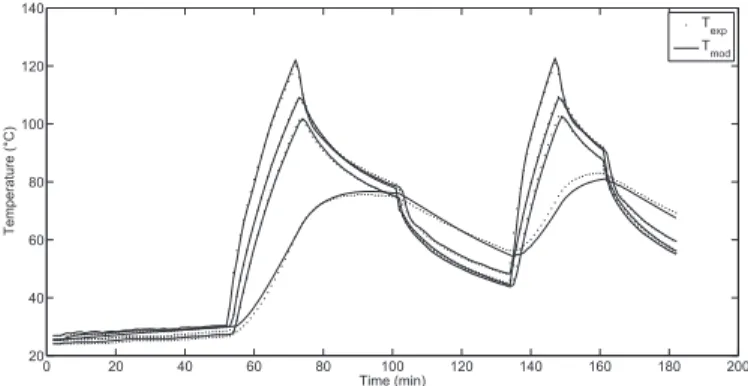
Figure 2 shows the results of evaluating these models with the same inputs as used in the real system to obtain the experimental data, for the four control volumes. Dots are the measured values and solid lines show the model results. From

0 20 40 60 80 100 120 140 160 180 200 20

40 60 80 100 120 140

Time (min)

Temperature (°C)

T_exp Tmod

Figure 2. Experimental data and initial ARX model

the top to the bottom, the sets correspond toT01,T06,T10and

T12, accordingly. Using the mean absolute percentage error, the

fitting of the model to the experimental data is96.6%,98.6%,

97.8% and 97.7%, respectively. The fitting of this model is adequate to the purpose of this paper and this is the model used to simulate the system in controller evaluation in Section V.

IV. CONTROL-ORIENTEDMODEL FACING THECONTROL

DESIGN

The model presented in Section III describes in a proper way the behavior of the system, but it poses some incon-veniences to the on-line optimization required for an MPC controller design. This fact motivates the development of a simpler model to ease the aforementioned calculation. This simpler model follows the same structure than the previous one but substitutes the Log Mean Temperature Difference

(LM T D), which mathematical expression is far from linear, for a simple temperature difference (∆T) between the inlet temperature to the control volume and the temperature of the fluid to which energy is transferred (reaction mixture or environment air). The reason LM T Dis used for modeling a heat exchanger is that the temperature difference is not uniform along the exchanger. But, since in an ARX model this variation can be absorbed by the calculated coefficients, this change in temperature difference expressions can be suitably made.

The orders of the polynomials obtained are (1,1,1) forp1,

p2 andj; and (1,3,1) forR. This model was validated as well

and the results obtained were quite alike those in Figure 2. By doing the substitution of LM T Dby∆T, the model becomes linear and it can be represented in the form [7]

x(k+ 1) =Ax(k) +Bu(k) +f, (11) wherex∈R8 is the state vector defined as

x = [T01(k), T01(k−1), T01(k−2), T06(k), T10(k),

T12(k), T12(k−1), T12(k−2)]T,

besides,u∈ U ⊆R2, whereU ,[0,1]2is the input vector de-fined asu= [H(k), cw(k)]T andf is an affine factor given by

CTe. Moreover, the outputs are:T01(k) =x(k){1},T06(k) =

0 50 100 150 200 0

20 40 60 80 100

T [°C]

T01 Ref

0 50 100 150 200

0 0.5 1

t [min]

u

H cw

Figure 3. Performance of preliminary on-line MPC

V. EMPC CONTROLLERDESIGN

Using the models described in Sections III and IV, some preliminary MPC controllers were developed, solving the on-line optimization problems using the fmincon function of MATLAB, TOMLAB optimization package for MATLAB [9] and the Multi-Parametric Toolbox 3 (MPT3) [10]. An hypo-thetical trajectory was established for the reference temperature to T01: starting from room temperature (25◦C), it is then

fixed at 60 ◦_{C during 90 minutes, then it shifts to 80}◦_{C for}

60 minutes and finally goes down to 40 ◦C. This trajectory replicates the one of a typical batch reaction in which the reactants are heated up for mixing, then they are further heated for the reaction to take place at steady temperature and finally they are cooled down for discharge. The results and analysis for those controllers are presented in [11].

The objective function that collects the control objectives for the case study has the form

J(k) =γ1

H_p

X

k=1

(T01(k)−T

r

01(k)) 2

+γ2

H_p

X

k=1

(u1(k)) +γ3

H_p

X

k=1 (u2(k)),

(12)

whereHp denotes the prediction horizon,T01r is the reference

trajectory and γi, for i={1,2,3}, are the weighting factors

that prioritize each term withing the multi-objective cost func-tion (12). For all these preliminary controllers,Hp = 10and

γ1 = γ2 = γ3 = 1. All the calculations were performed on

MATLAB R2013b (8.2.0.701) using a Windows 8 PC with Intel CORE i5 3337U, 6 GB RAM. The elapsed time for this controllers was 936.89 s (fmincon), 126.54 s (TOMLAB) and 180.5 s (MPT3). The results for the last of this controllers are shown in Figure 3.

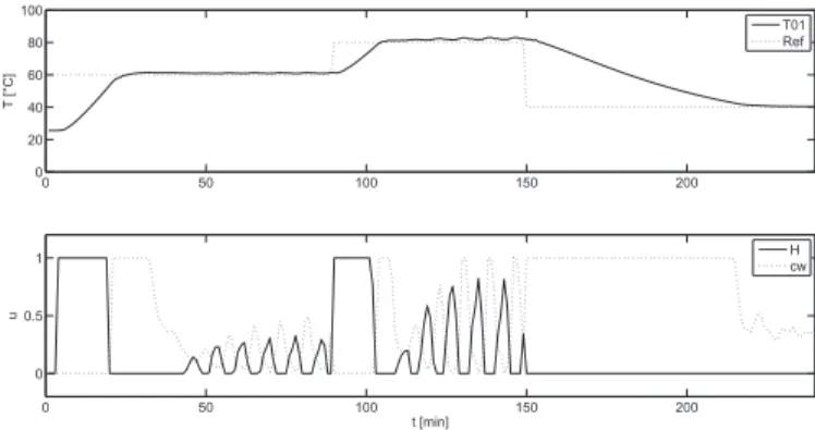
Then, an EMPC controller has been designed and simulated looking forward to obtaining a controller suitable to direct calculation by the existing PLC on the subject equipment. To attain that, the model used in the prediction stage of the MPC was further simplified by reducing its order on the previous section to (1,1,1) for all control volumes. Doing so, it resulted in a model of the same form as (11) but withx∈R4 defined as x = [T01(k), T06(k), T10(k), T12(k)]T. The quality of the

prediction slightly decreased but results are still similar to those in Figure 2 and this reduction in accuracy is mitigated by the feedback of the system measurements or simulation.

By using MPT3 for MATLAB [10], an EMPC is obtained for the (1,1,1)-order ARX model. To do this, the

optimiza-0 50 100 150 200

0 20 40 60 80 100

T [°C]

T01 Ref

0 50 100 150 200

0 0.5 1

t [min]

u

H cw

Figure 4. Performance of EMPC controller

tion problem is reformulated as a MP-QP –Multi Parametric Quadratic Programming– problem where the state space is divided into several regions when solving and for each one an explicit control law is formulated, as follows [12],[13]:

u=Fix+gi if Aix≤bi, (13)

whereF, g, Aandbare matrices of suitable dimensions given by the statement of the multi parametric optimization problem according to the formulation presented by [12],[13].

In addition, reference tracking can be enabled also by set-ting the reference as an additional parameter. It is then included as an additional element in the state vector x, resulting in

x = [T01(k), T06(k), T10(k), T12(k), T01ref(k)]T. The solution

for this problem, with Hp = 5 to prevent the problem size

from growing further, is composed of 38 regions. With a set of matricesF, g, A andbfor each region. These are not further detailed here because of space limitations. The results of using it to control the system are shown in Figure 4.

Despite the reference shifts are not previewed by the controller, both controllers achieve an acceptable reference tracking considering the nature of the system. The controlled variable(T01)reaches the reference quickly and with a small

overshoot. However, they show a small steady-state error that may be caused by the mismatch between simulation and control models. A summary of the key performance indexes (KPI) used to evaluate the performance of the closed loop with every designed controller, is presented in Table I. As expected, computational time is much less for the EMPC than for the MPC. Besides, EMPC shows a better general performance than on-line MPC. As for the objective function (12) with γi= 1,

EMPC yields a smaller sum of squared error, with softer changes and avoiding excessive heating and the subsequent need for additional cooling. This also reduces oscillation, as observed after time 100 minutes in Figure 3.

Table II shows some transient time performance indicators for the first and second steps in Figures 3 and 4. Rise times are quite similar since they are limited by the heating and cooling power of the equipment, not by the controller, as it can be noticed on the fact that both controllers keep heating (H) on until short before reaching the target temperature for the first time. Overshoot is higher for EMPC because it uses a shorter Hp in order to keep the number of regions in the

Table I. KPI COMPARISON

KPI MPC EMPC

Computational time [s] 180.5 0.9

Total cost function 55338 52047

Sum of squared error 55175 51905

Sum ofH 42.9 39.5

Sum ofcw 120.6 102.6

Table II. PERFORMANCE INDICATORS FOR EACH STEP

Step/Controller Rise Time [min]

Overshoot

[%]

Settling Time [min]

1st _{/ MPC 13.3 2.3 23.1}

1st _{/ EMPC 13.2 7.1 46.5}

2nd _{/ MPC 9.7 2.4 —}

2nd _{/ EMPC 10.1 2.8 48.5}

overshooting in comparison to the on-line MPC controller with a longer Hp. In addition, this higher overshoot makes the

settling time longer. Moreover, due to the oscillations in H

andcwcaused by the MPC,T01does not settle within the 5%

band in the second step when using the on-line MPC, as seen in Figure 3. In general, it can be said that EMPC has a better overall performance than MPC, under the conditions of this paper.

VI. CONCLUSIONS

This paper has presented and discussed the temperature control of a pilot-scale batch reaction system by means of the design of an explicit model predictive control (EMPC). A (1,1,1)-order ARX model has been developed to ease the calculations aiming at the implementation of the final controller on a existing PLC-based control system. An EMPC was obtained using MPT3 with this simplest model; it is composed of 38 regions and the results of using it to control the simulated system were good, though the reference shifts are no previewed by the controller. The controlled variable reaches the reference quickly and with a small overshoot. The changes on manipulated variables are softer than those of on– line optimization solutions. Some comparisons have been also performed with a traditional MPC computed online in order to see the potential differences in the system performance when a predictive-like control is computed on-line and off-line. Under the conditions of this study, the overall performance of the EMPC resulted better than that of the MPC.

The simple computation of control laws (only matrix sums and products), along with the still manageable number of regions and size of the matrices involved, makes it possible to implement the EMPC on the intended equipment, which is the subject of ongoing work. At the time of this publication, the EMPC described in section V had already been coded for the PLC on the real system using SIEMENS SCL programming language and its performance was about to be tested.

ACKNOWLEDGMENTS

The research of C. Ocampo-Martinez is partially supported by the Spanish project ECOCIS (Ref. DPI2013-48243-C2-1-R). The authors are glad to thank IRI for hosting this work, and Santander Universidades for funding it through its Becas Iberoam´erica J´ovenes Profesores e Investigadores 2013–2014 scholarship.

REFERENCES

[1] A. Sanz, A. Cardete, R. Lucio, R. Martinez, S. M. noz, D. Ruiz, C. Ruiz, O. Gerbi, and J. Papon, “Model-based predictive control increases batch reactor production,”Hydrocarbon Processing, no. 5, pp. 61–65, 2005. [2] P. Jarupintusophon, M. L. Lann, M. Cabassud, and G. Casamatia, “Reallistic Model-based Predictive and Adaptative Control of Batch Reactor,”Computers & Chemical Engineering, vol. 18, pp. S445–S449, 1994.

[3] Y. Ho, F. Mjalli, and H. Yeoh, “Multivariable adaptive predictive model based bontrol of a biodiesel transesterification reactor,” Journal of Applied Sciences, vol. 10, no. 12, pp. 1019–1027, 2010.

[4] S. Lucia, T. Finkler, D. Basak, and S. Engell, “A new robust NMPC scheme and its application to a semi-batch reactor example,” in Pro-ceedings of the 8th IFAC Symposium on Advanced Control of Chemical Processes, Furama, Riverfront, July 10–13 2012, pp. 69–74. [5] M. Bakosova, J. Oravec, and K. Matejickova, “Model predictive

control-based robust stabilization of a chemical reactor,” Chemical Papers, vol. 67, no. 9, pp. 1146–1156, 2013.

[6] V. Agarwal, M. Gupta, U. Gupta, and R. Saraswat, “A Model Predictive Controller Using Multiple Linear Models for Continuous Stirred Tank Reactor (CSTR) and its Implementation Issue,” inProceedings of the 4th International Conference on Communication Systems and Network Technologies, Bhopal, India, 7-9 April 2014.

[7] L. Ljung,System Identification: Theory for the User, 2nd ed. Upper Saddle River, N.J.: PTR Prentice Hall, 1999.

[8] ——, “System identification toolbox for use with MATLAB : user’s guide,” 1995.

[9] K. Holmstr¨om, “Tomlab – an environment for solving optimization problems in matlab,” inProceedings for the Nordic MATLAB Confer-ence ’97, 1997, pp. 27–28.

[10] M. Herceg, M. Kvasnica, C. Jones, and M. Morari, “Multi-Parametric Toolbox 3.0,” in Proceedings of the European Control Conference, Z ¨urich, Switzerland, July 17–19 2013, pp. 502–510.

[11] J. Sanchez and C. Ocampo-Martinez, “Temperature modelling and model predictive control of a pilot scale batch reaction system,” Institut de Rob`otica i Inform`atica Industrial (IRI), Tech. Rep. IRI-TR-03-14, September 2014.

[12] A. Bemporad, M. Morari, V. Dua, and E. Pistikopoulos, “The Explicit Linear Quadratic Regulator for Constrained Systems,” Automatica, vol. 38, no. 1, pp. 3–20, 2002.