Mean structure analysis from an irt approach: an application in the context of organizational psychology

Mean and covariance structure analysis comprises a set of statistical techniques that simultaneously deals with the means of the latent variables and the covariance structure. The factor model is possibly the most popular type of statistical model for this purpose. Its original formulation assumes that the means of the latent variables are null and

therefore neglects the mean structure analysis. Additionally, it assumes a linear relation between the observed variables and the factors, which implies that the observed variables are quantitative. However, later developments extended these models for the analysis of categorical data and the mean structure (Jöreskog & Sörbom, 2001).

Adding the mean structure implies that the observed means are summarized into a smaller number of latent means. The practical application of this analysis consists of comparing latent means across several groups of individuals while simultaneously investigating the pattern of covariance in a single statistical framework. This technique is meaningful when several variables measure one common characteristic.

Fecha recepción: 13-2-12 • Fecha aceptación: 7-7-12 Correspondencia: Javier Revuelta Menéndez Facultad de Psicología

Universidad Autónoma de Madrid 28049 Madrid (Spain)

e-mail: javier.revuelta@uam.es

Mean structure analysis from an IRT approach: An application

in the context of organizational psychology

Javier Revuelta Menéndez and Carmen Ximénez Gómez

The application of mean and covariance structure analysis with quantitative data is increasing. However, latent means analysis with qualitative data is not as widespread. This article summarizes the procedures to conduct an analysis of latent means of dichotomous data from an item response theory approach. We illustrate the implementation of these procedures in an empirical example referring to the organizational context, where a multi-group analysis was conducted to compare the latent means of three employee groups in two factors measuring personal preferences and the perceived degree of rewards from the organization. Results show that higher personal motivations are associated with higher perceived importance of the organization, and that these perceptions differ across groups, so that higher-level employees have a lower level of personal and perceived motivation. The article shows how to estimate the factor means and the factor correlation from dichotomous data, and how to assess goodness of fi t. Lastly, we provide the M-Plus syntax code in order to facilitate the latent means analyses for applied researchers.

Análisis de estructura de medias mediante un modelo TRI: una aplicación en el contexto de la psicología de las organizaciones. La aplicación de modelos de análisis de estructura de medias y covarianzas en datos cuantitativos está extendiéndose. Sin embargo, el análisis de medias latentes a partir de datos cualitativos es menos habitual. Este artículo resume los procedimientos para llevar a cabo un análisis de estructura de medias latentes con ítems dicotómicos desde un enfoque de la teoría de respuesta al ítem. Se ilustra la implementación de dichos procedimientos en un ejemplo con datos empíricos referidos al contexto organizacional, donde se lleva a cabo un análisis multi-grupo para comparar las medias latentes de tres grupos de empleados en dos factores que miden preferencias personales y el grado percibido en que la organización las refuerza. Los resultados indican que a mayor motivación personal, se necesita mayor refuerzo por parte de la organización, y que existen diferencias entre grupos, ocurriendo que los empleados que ocupan posiciones más altas tienen menor nivel de motivaciones personales y organizacionales. El artículo muestra cómo estimar las medias y correlaciones de los factores de ítems dicotómicos, y cómo evaluar la bondad de ajuste. Por último, se muestra la sintaxis M-Plus para facilitar la aplicación de este tipo de análisis a los investigadores.

Several theoretical studies have noted the advantages of adding the analysis of the mean structure in the factor model. Yung and Bentler (1999) found that in maximum likelihood factor analysis the reduction of asymptotic variances for factor loadings can be quite substantial when a mean structure is added. Yuan and Bentler (2006) found that summarizing observed variables into latent means conveys an increase of statistical power when null hypothesis signifi cance testing is used to compare means across groups. Finally, another advantage of adding the associated mean structure is that the model accounts for measurement error variances in estimating the latent means whereas this is not possible in the techniques that compare the observed means (e.g., T-test and ANOVA).

Given these advantages, the application of factorial models simultaneously analyzing the mean and covariance structure for quantitative variables is increasingly growing and several empirical studies use this approach. However, the latent means analysis with qualitative data is not as widespread. Particularly, because the use of dichotomous data implies that the linear model is not well suited to approximate the relation between the observed and the latent variables and instead, models are based in a nonlinear function (e.g., an item response theory model, IRT) and the interpretation of the latent means is based on their relation with the probability of the response categories, instead of the relation with the values of the observed variables as in the linear model.

The aim of this article is to explain the procedures to conduct a mean structure analysis of dichotomous data from an IRT approach in the one-dimensional case. Despite IRT models are well known, they are seldom used to compare latent means between groups. This is due to two reasons: First, the mean structure analysis requires the assumption of certain theoretical constraints, both in the item parameters and in the means. Second, the estimation of these models requires and advance use of the computer programs. With this article, we pretend to clarify both issues to facilitate the use of these models for applied researchers.

The article is organized as follows. First, we explain the IRT with mean structure model, its relation with the factor model, and how the interpretation of the latent means is based on the probabilities of the response outcomes. Second, we explain the necessary constraints to be imposed in the IRT model for the estimation of the latent means and the problem of the factorial invariance so that the comparison of the latent means across groups is meaningful. Finally, we illustrate the implementation and interpretation of these procedures in an empirical example taken from the organizational context and provide the M-Plus syntax code for these analyses, which are less known by researchers.

Item response theory model with mean structure

The common factor model with mean structure is defi ned by (Sörbom, 1981):

x= τ_x + Λξ + δ, (1)

where x is a vector of p observed variables, τ_x is a vector of p constant intercept terms, ξ is a factor or latent variable, Λ is a vector of factor loadings, and δ is a vector of p measurement errors. It is assumed that E(δ)= 0 and E(ξδ)= 0; However, E(ξ) is not 0, it is a parameter denoted by κ. By taking the expectations of Equation (1), the mean vector of the observed variables is:

E(x)= τ_x + Λκ (2)

Certain constraints need to be imposed for the estimation of parameters. For instance, λ_ij is set to 1 and its corresponding τ_x

i to 0, so that the factor has the same measurement scale than X_i and the same mean: E(X_i)= κ. This constraint makes possible the comparison of the latent means across groups, but only when Λ is invariant across groups, which guaranties that the factors have the same measurement scale for each group.

Social scientists usually do not work with quantitative data. For instance, items from attitude scales are usually scored in a small number of categories, such as right or wrong responses. In these cases, the linearity assumption of the factor model is only an approximation to the relation between factors and scores. The categorical factor analysis, usually referred to as item factor analysis (Bock & Gibbons, 2010; Wirth & Edwards, 2007), assumes that observed data originate from a discretization of an underlying quantitative variable. Consider the linear factor model defi ned in Equation (1). The item factor model for dichotomous data assumes that x_i is a latent variable and the observed responses arise by categorizing xi into two response categories using one threshold value. The variable x_i is converted into the observed variable r_i according to the transformation:

r_i= 0, ifxii 1, ifx_i>_i

where x_i= λ_iξ + δ_i and the threshold υ_i is a new parameter that needs to be estimated. For convenience, the model assumes that the distribution of x_i conditional on ξ, referred to as f_i(x), is normal with mean λ_iξ and variance 1-λ2

i. Given a fi xed value of ξ, the probability that ri falls in the category 1 is the area under the normal curve that lies above the threshold. If φ(z) is a standard normal density function, then:

i=P x

(

)

i

(x)dx= (z)

ii

1_i2

dz=

ii

1_i2

(z)dz

This model is also referred to as a normal ogive model. The two-parameter logistic model from IRT (Hambleton & Swaminathan, 1985) may be seen as a transformation of the item parameters λi and υi into the ai and bi parameters to facilitate interpretation, where a_i is a scale parameter that indicates the ratio of change of π_i in relation to ξ, and b_i is a diffi culty parameter that indicates the value of ξ that has a probability 0.50 of endorsing the item. The relation between the parameters of the common factor model and the IRT parameterization is given by (Ferrando, 1996):

a_i= i

1i2

b_i=i

i

i= (z) a_i(bi)

dz exp

(

)

1+exp

₍

₎

(4) where D=1.70. However, we will omit D because it is not necessary to improve model-data fi t. When the data are dichotomous, the interpretation of factor means is based on their relation with the probability of the response categories, instead of the relation with the values of the observed variable as in the linear model.

IRT models also have a problem of indeterminacy of the scale of the factors, which is resolved by setting some parameters to constant values so that the model is identifi ed (Revuelta, 2009). More specifi cally, the diffi culty parameter for one of the items is set to zero (b1= 0) so that the factor mean can be estimated without increasing the number of parameters. The value of κ is interpreted in relation to the probability of endorsing the fi rst item. Given that b₁= 0, then π₁= exp(a₁ξ) / (1 + exp(a₁ξ)) and the factor is function of the odds of endorsing the item:

log 1

1₁

1/ a₁

=

(5) Thus, κ is the population mean value of function (5). As this function increases with π₁, the high values of κ are associated to a higher probability of endorsing Item 1. Additionally, a₁ can be fi xed to a constant value, say 1, for estimating the variance of the factor.

These constraints allow the estimation of the factor mean and variance in the single group case. In multi-group designs the aim is to compare factor means across groups. This is meaningful if a_i and bi are invariant across groups. Only if the invariance is achieved, any given trait level has associated the same response probability in all groups and therefore, if the mean in a group is larger than in the other, this implies a larger probability of responses in the category 1 for the group with the largest mean. Invariance is satisfi ed when all the items have the same a_i and b_i across groups. As this constraint is very restrictive, in practice partial invariance models are fi tted, which impose the invariance constraints in certain subset of variables.

The practical implementation of a latent mean analysis requires two steps: 1) the analysis of the invariance across groups; and 2) the latent means comparison. Step 1 is carried out by comparing the goodness of fi t of models of full invariance, partial invariance and non-invariance to determine if there is some degree of invariance that makes possible the latent means comparison. Provided that there is some degree of invariance, in Step 2 the latent means and variances are compared assuming that the same constraints in ai and b_i have been imposed across all the groups.

In multi-group studies it is common to assume that the means of the groups are a linear function of the parameters that indicate if there are main or interaction effects, similar as in log-linear analysis (Agresti, 2002) and ANOVA models (Rencher & Schaalje, 2008). For example, in a design with two independent variables, the mean of each cell of the design is denoted by:

jl=+ j+l+jl, ₍₆₎

where j and l are the levels of each independent variable, α_j and βl are the main effects, and γjl is the interaction effect. These

parameters are constrained to sum 0 and are expressed as linear combinations of a set of parameters, named basic parameters. For example, in a 2×3 design the cell parameters are expressed as a function of six basic parameters, δ₁ to δ₆, as follows:

κ11= δ1+ δ2 + δ3+ δ5 κ21= δ1 – δ2 + δ3 – δ5

κ12= δ1+ δ2 + δ4 + δ6 (7) κ₂₂= δ₁ – δ₂ + δ₄ – δ₆

κ31= δ1+ δ2 – δ3 – δ4 – δ5 – δ6 κ32= δ1 – δ2 – δ3 – δ4 + δ5 + δ6 The parameters of model (6) are given by:

μ= δ₁,

α₁= δ₂, α₂= – δ₂

β₁= δ₃, β₂= δ₄, β₃= –δ₃ –δ₄

γ11= δ5, γ12= δ6, γ13= –δ5 – δ6

γ₂₁= –δ₅, γ₂₂= –δ₆ and γ₂₃= δ₅ + δ₆

This parameterization implies that the sum of the effects is zero. That is:

j j

=0, _l

l

=0, _jl

j

=0 and _jl

l

=0

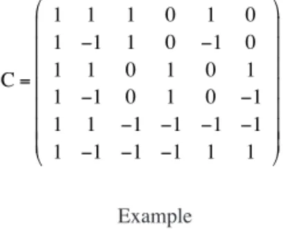
In matrix notation, the vector of factor means is: κ= Cδ,

where C is a constant matrix that specifi es the effects assessed in the model and must have full column rank. For instance, the C matrix for Equation (7) is:

C=

1 1 1 0 1 0

1 1 1 0 1 0

1 1 0 1 0 1

1 1 0 1 0 1

1 1 1 1 1 1

1 1 1 1 1 1

Example

A questionnaire of Person-Organization (P-O) fi t was analyzed to illustrate the analysis and interpretation of latent means with dichotomous data.

Participants. A sample of 566 participants was recruited from former university students. 260 were men and 306 were women, and their average age was 35 years (standard deviation: 6.21). Three groups were defi ned according to the positions of the participants in their organizations. Sample 1 with 216 employees working in low-level positions, Sample 2 with 248 employees working in middle-level positions, and Sample 3 with 102 high-middle-level directors.

based in the MJDQ (Borgen et al., 1972). Both questionnaires are independent and were administered separately.

Statistical analyses. The estimated parameters are the factor loadings, the thresholds, the latent means and variances, and the factor correlations. Factor loadings and thresholds are constant across groups, whereas the other parameters depend on the model. Four models were applied that differ in the constraints imposed: Model 1: no constraints across groups; Model 2: factor correlations equal across groups; Model 3: factor means equal across groups; and Model 4: factor means and correlations equal across groups.

Models were estimated using M-Plus 4.1 (Múthen & Múthen, 2006). This program provides the values of the categorical factor analysis parameters: υi, λi, κ, and φ, which were transformed into the IRT parameters a_i and b_i by using Equation (3). Table 2 shows the M-plus syntax code for the estimation of Model 1. The equations defi ned in (7) are implemented in lines 59 to 64. The parameters δ₁ to δ₆ are denoted by C1 to C6, and are defi ned in line 54. The constraints defi ned in the other models can be easily implemented by modifying the syntax code. The general procedure consists of assigning a label to the parameters of the factor model (see lines 15 to 50, where all terms in brackets are labels), defi ning the basic parameters (lines 52 to 54), and specifying the calculation of the parameters of the factorial model from the basic parameters (lines 55 to 64).

The ULS estimation method was used because the other methods are not appropriate for the data of the example (ML uses information of the response patterns and there are very few in the example, WLS uses the asymptotic covariance matrix and it can not be estimated with small sample sizes, and GLS requires normality). We did not calculate the chi-square difference for hierarchical models because it is not possible with ULS (see Technical appendices in the URL: www.statmodel.com to compute this statistic with other estimation methods).

One important concern in this context is to obtain comparable factor scores on the P and O scales. This is achieved when both scales have the same thresholds and factor loadings for every pair of items, one for each scale (Ximénez & Revuelta, 2010). As previous analysis showed evidence that this assumption is too restrictive, a partial measurement invariance approach (Byrne, Shavelson, & Muthén, 1989) was taken. Items 1 to 5 were regarded as an anchor test (von Davier, 2010) with the purpose of obtaining commensurate factor scales for the P and O factors, and thus their parameters were set to be equal on the two scales. Items 6 to 15 were left free to vary from one scale to the other.

The example corresponds to a 2×3 mixed design with one within-subjects independent variable (with levels P and O) and one between-subjects independent variable (with the three levels of employees), that could be solved with an ANOVA if we analyze the effects on the observed means. The difference with the IRT approach is that the aim of the latter is studying the effects on the latent means.

Results. Table 3 contains the goodness of fi t indices chi-square (χ2_{) and RMSEA for each model. The results showed that all models} fall short of being acceptable and imposing constraints conveys a decrease in model fi t compared with the less restrictive model. For these reasons, the best fi tting model (Model 1) was selected for interpretation.

Parameter estimates appear in Table 4, which follows the notation of Figure 1. As can be seen, the estimates from every pair of matched items were different when they were allowed to vary (in items 6 to 15), indicating that the reaction towards any given item stem is not the same when it refers to personal or to organizational Table 1

Description of items

Code Description

P1/O1* _{My rewards compare well with those of others}

P2/O2 My group leader provides for my continuing membership P3/O3 My group leader backs me up

P4/O4 My group leader communicates expectations well P5/O5 I can make decisions on my own

P6/O6 I can try out my own ideas P7/O7 I can plan things independently

P8/O8 People at my work are easy to make friends with P9/O9 I can do things for other people

P10/O10 I can be busy all the time

P11/O11 I can do something different every day P12/O12 I can get a feeling of accomplishment P13/O13 I can have the opportunity for self-advancement P14/O14 I can receive recognition for the things I do P15/O15 I can be somebody in the group

* _{Items P1 to P15 were answered in terms of “for me it is important that …”, whereas items}

O1 to O15 were answered in terms of “for my organization it is important that …”

P O P1 P2 P3 P4 P5 P6 P7 P8 P9 P10 P11 P12 P13 P14 P15 O1 O2 O3 O4 O5 O6 O7 O8 O9 O10 O11 O12 O13 O14 O15 δ_P1 δ_P2 δ_P3 δ_P4 δ_P5 δ_P6 δ_P7 δ_P8 δ_P9 δ_P10 δ_P11 δ_P12 δ_P13 δ_P14

δ_P15 δ_O15

δ_O14 δ_O13 δ_O12 δ_O11 δ_O10 δ_O9 δ_O8 δ O7 δ O6 δ O5 δ_O4 δ_O3 δ_O2 δ_O1 0 υ_P2 υ_P3 υ_P4 υ P5 υ P6 υ P7 υ_P8 υ_P9 υ_P10 υ_P11 υ_P12 υ_P13 υ_P14 υ_P15 υ_O2 υ_O3 υ_O4 υ O5 υ O6 υ O7 υ_O8 υ_O9 υ_O10 υ_O11 υ_O12 υ_O13 υ_O14 υ_O15 0 λ_P1 λ_P2 λ_P3 λ_P4 λ_P5 λ_P6 λ_P7 λ_P8 λ_P9 λ_P10 λ_P11 λ_P12 λ_P13 λ_P14 λ_P15 λ_O1 λ_O2 λ_O3 λ_O4 λ_O5 λ_O6 λ_O7 λ O8 λ O9 λ_O10 λ_O11 λ_O12 λ_O13 λ_O14 λ_O15 κ_P κ_O

φ_PO

values. The table also shows that factor mean was consistently higher for P than for O, indicating that the employees exhibited a

lack of fulfi llment of their personal values. Moreover, as the level in the organization decreases the difference between the means of personal and organizational values increased. This is refl ected in which the interaction parameters are signifi cantly different from zero (δ₅= -0.19, Se= 0.08, Z= -2.40; and δ₆= 0.20, Se= 0.08, Z= 2.63). Finally, there was a positive correlation between factors, indicating that employees with high expectations scored higher on the scale of organizational values, which increased with the level in the organization.

As a comparison, if this research problem was solved by an ANOVA the independent variable is the score in the P and O scales, and would be obtained by adding their 15 items. This implies a mixed design with Position (low, medium, and high) as a between-subjects factor and Scale (P and O) as a within-subjects factor. The means of P for the low, medium and high positions are 11.53, 11.35, and 11.61; the means of O are 4.09, 4.71, and 5.75. Both the main and the interaction effects were signifi cant, and the correlations between P and O in each group were .07, .30, and .35. Thus, the conclusions are equal with the IRT and ANOVA approaches; however, the information that is missed with the ANOVA is the analysis of dimensionality, the relation of P and O with the individual scores in each item and the measurement errors.

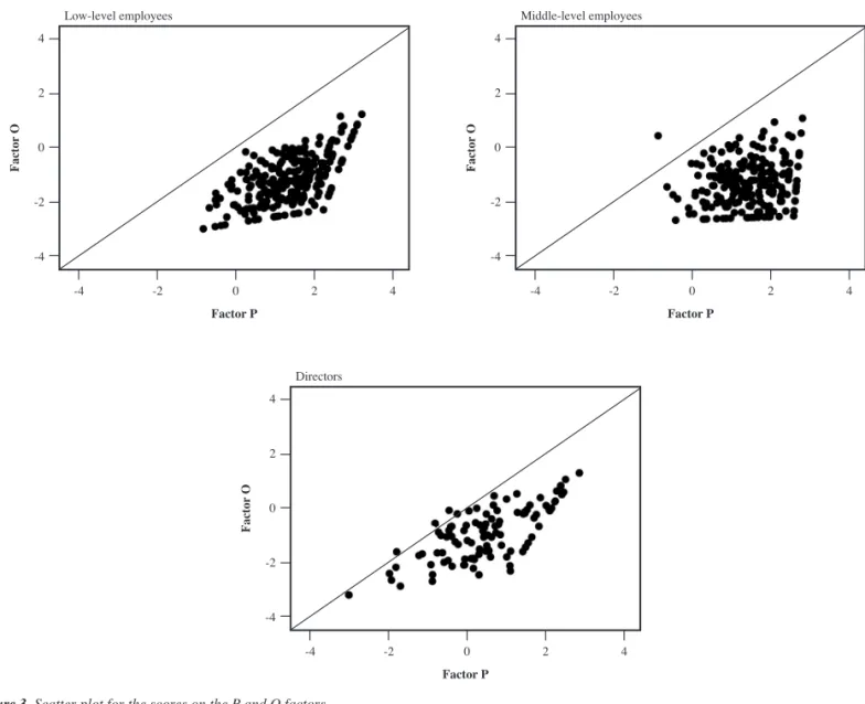
Figure 2 provides further insight. It contains the item characteristic curves for all the items of P and O. Conditional on the factor value, there is a higher probability of endorsing items on the O scale than the matched items on the P scale. The fi gure also contains the distribution of the factor scores, which showed a shift to the right for the distribution of P because of its higher mean.

Finally, Figure 3 contains the scatter plot for the estimated factor scores. The diagonal line in the fi gure is the bisection line, which corresponds to equality between P and O scores. For almost all individuals the P score was higher than the O score, and thus the points fall in the lower right part of the fi gure. Two customary measures of P-O fi t applied to these data (Edwards, 1993) are d₁= Mean(|P – O|) and d₂= Mean((P – O)2_{). The values of d}

1 for the total group and the three subgroups were 2.63, 2.78, 2.58, and 2.43; and the values of d₂ were 7.72, 8.86,7.27, and 6.42, indicating that as the level in the organization decreased the degree of mismatch between personal and organizational values increased.

These results lead to two conclusions. First, the individuals feel that their motivations towards their workplaces are not suffi ciently fulfi lled by the organizations they work in. The mean value of P is consistently higher across groups and there is a positive correlation between P and O, so that higher personal motivations are associated with higher perceived importance by the organization. Second, Table 2

M-Plus syntax code 1 TITLE: Categorical factor analysis with a mean structure and 2 constraints

3 DATA: 4 FILE IS “PO.dat”; 5 VARIABLE:

6 NAMES ARE g p1-p15 o1-o15; 7 CATEGORICAL ARE p1-p15 o1-o15;

8 GROUPING IS g (1=directivos 2=administrativos 3=medios); 9 ANALYSIS:

10 TYPE IS MEANSTRUCTURE; 11 ESTIMATOR=ULS; 12 ITERATIONS=5000; 13 CONVERGENCE=0.00005; 14 MODEL:

15 f1 BY p1*(PA1) 16 p2(PA2) 17 p3(PA3) 18 p4(PA4) 19 p5(PA5) 20 p6-p15; 21 f2 BY o1*(OA1) 22 o2(OA2) 23 o3(OA3) 24 o4(OA4) 25 o5(OA5) 26 o6-o15; 27 [p1$1@0 o1$1@0]; 28 [p2$1](PB2); 29 [p3$1](PB3); 30 [p4$1](PB4); 31 [p5$1](PB5); 32 [o2$1](OB2); 33 [o3$1](OB3); 34 [o4$1](OB4); 35 [o5$1](OB5); 36 f1@1 f2@1; 37 [f1* f2*]; 38 f1 WITH f2 ; 39 MODEL directivos: 40 f1@1 f2@1; 41 [f1*0](MD1); 42 [f2*0](MD2); 43 MODEL administrativos: 44 f1@1 f2@1; 45 [f1*0](MA1); 46 [f2*0](MA2); 47 MODEL medios: 48 f1@1 f2@1; 49 [f1*0](MM1); 50 [f2*0](MM2); 51 MODEL CONSTRAINT:

52 NEW(A1);NEW(A2);NEW(A3);NEW(A4);NEW(A5); 53 NEW(B2);NEW(B3);NEW(B4);NEW(B5);

54 NEW(C1);NEW(C2);NEW(C3);NEW(C4);NEW(C5);NEW(C6); 55 PA1=A1; PA2=A2; PA3=A3; PA4=A4; PA5=A5;

56 OA1=A1; OA2=A2; OA3=A3; OA4=A4; OA5=A5; 57 PB2=B2; PB3=B3; PB4=B4; PB5=B5;

58 OB2=B2; OB3=B3; OB4=B4; OB5=B5; 59 MD1=C1+C2+C3+C5;

60 MD2=C1-C2+C3-C5; 61 MA1=C1+C2+C4+C6; 62 MA2=C1-C2+C4-C6; 63 MM1=C1+C2-C3-C4-C5-C6; 64 MM2=C1-C2-C3-C4+C5+C6; 65 SAVEDATA:

66 FILE=scores4.dat;

Table 3

Goodness of fi t statistics

Invariance fp df χ2 _{p RMSEA}

Model 1 118 126 166.1 .010 .041

Model 2 116 119 162.4 .005 .044

Model 3 114 125 167.7 .007 .043

Model 4 112 118 164.9 .003 .046

Note: fp is the number of free parameters, df is the degrees of freedom, χ2 _{is the chi-square}

goodness of fi t statistic, p is the probability associated to χ2_{, and RMSEA is the root mean}

these perceptions differ across groups, so that the employees with higher-level positions have a lower level of personal and a higher level of perceived motivation.

Discussion and conclusion

The analysis of latent means allows summarizing the means of several observed variables in a smaller number of factor means that can be compared across groups. This reduction of information is meaningful when the observed variables measure a common attribute and it provides parsimony in the statistical analysis. Other advantages of the analysis of latent means are: 1) it allows the analysis of the covariance structure and latent mean differences across groups to be carried out simultaneously within a single integrated statistical framework; 2) it accounts for measurement error variances in estimating the latent means whereas ANOVA does not take into account this source of variance; and 3) these models have desirable statistical properties as summarizing observed means into latent means conveys an increase of statistical power when null hypothesis signifi cance testing is used to compare means across groups.

The factorial model is appropriate to compare latent means with quantitative variables. However, the majority of data found in practice are categorical, and this may require an IRT model that allows the analysis of latent means for categorical data. These models present more diffi culties because the relation between factors and observed variables is not as straightforward as in the quantitative model as it is interpreted with the probability of the response outcomes associated to each category.

This article has focused in the dichotomous case analyzed by an IRT model. At a theoretical level, it have been shown how to set certain parameters to constant values to estimate and interpret the factor means. More specifi cally, one diffi culty parameter is set to zero and therefore, the factor mean depends on the probability of endorsing that item. Additionally, the article shows how to impose linear constraints in the latent means to assess both main and interaction effects.

At a practical level, the article illustrates the procedure with an example taken from the organizational context, where a multi-group analysis was conducted to compare the latent means of three employees groups in two factors measuring personal preferences and the perceived degree to which the organization rewards them. The example shows how to estimate the factors working with dichotomous data, how to correlate them, assess the goodness of fi t, and compare their latent means. The analysis of latent means from an IRT approach has the problem that the majority of computer software does not allow to estimate them and the programs that do so require a complex syntax. In this article, we have shown how to implement such analyses with a well known program as is the M-Plus and how to defi ne the parameter constraints. An M-Plus syntax code has been included so that readers can adapt it to their own problems.

Acknowledgement

This work was partially supported by grant CCG08-UAM/ESP-3951 of the Comunidad of Madrid (Spain) and grant PSI2009-08264 of the Spanish Ministry of Science and Innovation. Table 4

Parameter estimates for Model 1

Scale P Scale O

Item υ λ a b υ a a b

01 -0.00 0.71 1.02 -0.00 -0.00 0.71 1.02 -0.00

02 -0.34 0.40 0.44 -0.84 -0.34 0.40 0.44 -0.84

03 -0.24 0.62 0.80 -0.38 -0.24 0.62 0.80 -0.38

04 -0.37 0.66 0.88 -0.55 -0.37 0.66 0.88 -0.55

05 -0.63 0.74 1.09 -0.85 -0.63 0.74 1.09 -0.85

06 -0.32 0.84 1.52 -0.39 -0.41 0.79 1.27 -0.52

07 -0.51 0.47 0.54 -1.07 -0.61 0.69 0.96 -0.87

08 -0.04 0.24 0.24 -0.16 -0.13 0.60 0.76 -0.21

09 -0.01 0.59 0.73 -0.02 -0.43 0.76 1.18 -0.56

10 -0.14 0.15 0.15 -0.95 -0.78 0.48 0.54 -1.64

11 -0.06 0.04 0.04 -1.50 -0.10 0.49 0.56 -0.21

12 -0.87 0.53 0.63 -1.64 -1.46 0.66 0.87 -2.21

13 -0.44 0.35 0.37 -1.24 -0.09 0.73 1.08 -0.12

14 -0.68 0.70 0.99 -0.97 -0.03 0.80 1.35 -0.03

15 -0.73 0.53 0.62 -1.39 -0.11 0.79 1.27 -0.13

Mean of the factor:

Low-level employees 1.61 -1.48

Middle-level employees 1.40 -1.28

Directors 1.35 -0.95

Variance of the factor: 1.00 -1.00

1,0 0,8 0,6 0,4 0,2 0,0

-5 -4 -3 -2 -1 0 1 2 3 4 5

Item 1

1,0 0,8 0,6 0,4 0,2 0,0

-5 -4 -3 -2 -1 0 1 2 3 4 5

Item 3

1,0 0,8 0,6 0,4 0,2 0,0

-5 -4 -3 -2 -1 0 1 2 3 4 5

Item 2

1,0 0,8 0,6 0,4 0,2 0,0

-5 -4 -3 -2 -1 0 1 2 3 4 5

Item 4

1,0 0,8 0,6 0,4 0,2 0,0

-5 -4 -3 -2 -1 0 1 2 3 4 5

Item 5

1,0 0,8 0,6 0,4 0,2 0,0

-5 -4 -3 -2 -1 0 1 2 3 4 5

Item 1

1,0 0,8 0,6 0,4 0,2 0,0

-5 -4 -3 -2 -1 0 1 2 3 4 5

Item 7

1,0 0,8 0,6 0,4 0,2 0,0

-5 -4 -3 -2 -1 0 1 2 3 4 5

Item 9

1,0 0,8 0,6 0,4 0,2 0,0

-5 -4 -3 -2 -1 0 1 2 3 4 5

Item 10

1,0 0,8 0,6 0,4 0,2 0,0

-5 -4 -3 -2 -1 0 1 2 3 4 5

Item 11

1,0 0,8 0,6 0,4 0,2 0,0

-5 -4 -3 -2 -1 0 1 2 3 4 5

Item 8

1,0 0,8 0,6 0,4 0,2 0,0

-5 -4 -3 -2 -1 0 1 2 3 4 5

Item 12

1,0 0,8 0,6 0,4 0,2 0,0

-5 -4 -3 -2 -1 0 1 2 3 4 5

Item 13

1,0 0,8 0,6 0,4 0,2 0,0

-5 -4 -3 -2 -1 0 1 2 3 4 5

Item 14

1,0 0,8 0,6 0,4 0,2 0,0

-5 -4 -3 -2 -1 0 1 2 3 4 5

Item 15

Figure 2. Item response functions and distribution of the factor scores for the P and O scales

4

2

0

-2

-4

Low-level employees

-4 -2 0 2 4

Factor P

Factor

O

4

2

0

-2

-4

Middle-level employees

-4 -2 0 2 4

Factor P

Factor

O

4

2

0

-2

-4

Directors

-4 -2 0 2 4

Factor P

Factor

O

Figure 3. Scatter plot for the scores on the P and O factors

References

Agresti, A. (2002). Categorical data analysis. New York. Wiley.

Bock, R.D., & Gibbons, R. (2010). Factor analysis of categorical item responses. In M.L. Nering & R. Ostini (Eds.), Handbook of polytomous item response theory models. New York, NY: Routledge.

Borgen, F.H., Weiss, D.J., Tinsley, H.E.A., Dawis, R.V., & Lofquist, L.H. (1972). Occupational reinforcer patterns. Minneapolis, MN: Vocational Psychology Research, University of Minnesota.

Byrne, B.M., Shavelson, R.J., & Múthen, B. (1989). Testing for the equivalence of factor covariance and mean structure: The issue of partial measurement invariance. Psychological Bulletin, 105, 456-466. Edwards, J.R. (1993). Problems with the use of profi le similarity indices

in the study of congruence in organizational research. Personnel

Psychology, 46, 641-665.

Ferrando, P.J. (1996). Relaciones entre el análisis factorial y la teoría de respuesta a los ítems [relations between factor analysis and item response theory]. Madrid: Universitas.

Gay, E.G., Weiss, D.J., Hendel, D.D., Dawis, R.V., & Lofquist, L.H. (1971). Manual for the Minnesota Importance Questionnaire. Minnesota Studies in Vocational Rehabilitation, 28.

Hambleton, R.K., & Swaminathan, H. (1985). Item response theory:

Principles and applications. Boston, MA: Kluwer.

Jöreskog, K., & Sörbom, D. (2001). LISREL 8. User’s reference guide. Lincolnwood, IL. Scientifi c Software International.

Múthen, L.K., & Múthen, B.O. (2006). MPLUS. Statistical analysis

with latent variables: User’s guide. Los Angeles, CA: Muthén and Muthén.

Rencher, A.C., & Schaalje, G.B. (2008). Linear models in statistics. New York: Wiley.

Revuelta, J. (2009). Identifi ability and equivalence of GLLIRM models.

Psychometrika, 74, 257-272.

Sörbom, D. (1981). Structural equation models with structured means. In K.G. Jöreskog & H. Wold (Eds.), Systems under indirect observation:

Causality, structure and prediction. Amsterdam: North-Holland Publishing Co.

von Davier, A. (2010). Statistical models for test equating, scaling, and linking. New York, NY: Springer.

Wirth, R.J., & Edwards, M.C. (2007). Item factor analysis. Current approaches and future directions. Psychological Methods, 12, 58-79.

Yuan, K.H., & Bentler, P.M. (2006). Mean comparison: Manifest variable versus latent variable. Psychometrika, 71, 139-159.

Yung, Y.-F., & Bentler, P.M. (1999). On added information for ML factor analysis with mean and covariance structures. Journal of Educational and Behavioral Statistics, 24, 1-20.

Ximénez, C., & Revuelta, J. (2010). Factorial invariance in a repeated measures design: An application to the study of person-organization fi t.