Some simple graphical interpretations of the Herfindahl Hirshman index and their implications

Texto completo

(1)Some Simple Graphical Interpretations of the Herfindahl-Hirshman Index and their Implications by Richard Watt and Javier de Quinto Universidad Autónoma de Madrid and Universidad San Pablo CEU. Abstract. This paper considers the Herfindahl-Hirshman (H) index for analysing industrial concentration in oligopoly markets. We find two new geometric interpretations of the index that have several implications as to the way in which mergers between firms in oligopoly markets will affect the value of the index. We show that, as other authors have argued, strict reliance upon the H index can indeed lead to incorrect policy concerning anti-trust issues if the true policy objective is social welfare. Furthermore, we show that there exist other measures, that do not require any more information than what the H index requires that avoid these problems. Key Words and Phrases: Herfindahl-Hirshman index, mergers, oligopoly. 1.

(2) 1. Introduction. Mergers between firms in oligopoly industries often inspire intense debate between economists, newspaper reporters, government officials, and consumers. A merger will generally imply transfers of large sums of money, as well as causing important changes in capital and labor markets. Naturally, there will also be significant effects on the production of goods and services, and their prices. Each of these effects implies changes in the welfare of many consumers, workers, investors, producers of substitute and complementary goods, and the treasury department. In principle, a merger should be judged to be “socially favorable” if the aggregate effect on social welfare is positive, and “socially un-favorable” otherwise. However, social welfare, and changes in social welfare, are impossible to calculate, or at best, require significant value judgements as to which members of society should weigh more heavily in the social welfare calculation. Consequently, decisions regarding mergers made on behalf of a society often inspire heated debate. In all developed economies, there exist antitrust commissions that pass judgement upon the social favorability of proposed mergers. For example, in the United States, the Department of Justice evaluates proposed mergers according to their anticipated effects upon competition and the creation of monopoly power. The basic guidelines upon which the final decisions are based are contained in a document that was first published in 1982, and then revised in 1984 and again in 1992 (see Salop (1987), White 2.

(3) (1987), Fisher (1987) and Schmalensee (1987) for a discussion of this document). Aside from considerations regarding the contestability of the market, the guidelines are heavily dependent upon the anticipated effects of a merger on the HerfindahlHirshman index (here-in-after denoted by H). For example, a merger that leaves the market with a value of H below 1,000 should not be opposed, while a merger that leaves the market with a value of H that is greater than 1,800 should always be opposed. If the merger leaves the market with a value of H between 1,000 and 1,800, it will only be opposed if it causes H to increase by more than 100 points. However, in general, it is impossible to express social welfare as a monotone function of H, and so guidelines that are based strictly on H may well lead to socially favorable mergers meeting with strong opposition, or socially un-favorable mergers to be passed. In contrast to guidelines based on the measure H, economists tend to evaluate the social effects of mergers by how they affect social welfare, or the sum of consumer and producer surplus, which we will denote by M. Given a market demand curve, M can be calculated once a model of how the firms that are active in the market compete has been established. Naturally, models based on different assumptions as to how the market operates will generally give different values for M , because they give different values of total production and of how this total production is distributed among the firms. One of the most curious aspects of the use of the H index in practically all of the. 3.

(4) antitrust debates concerning mergers is the absolutely naive manner in which it is used. The usual approach used by competition authorities consists in calculating the value of H before the merger, and then recalculating it after the merger assuming that the share of the merged entity equals the addition of the shares of the pre-existing firms, and that the shares of all other firms (those that do not participate in the merger) remain constant. This is obviously a severe abstraction from all reality, as any model of competition clearly reveals - a merger will necessarily affect the final market shares of all firms. It is very simple to show that the naive method always results in an increase in the value of H after a merger. However, being more realistic, one should contrast the pre-merger and the post-merger situations in terms of the equilibrium market shares in each case, which requires the application of an economic model of industrial competition. The result is that, in reality it is not true that a merger will always increase the value of H. In this paper we use a model of quantity competition known as the “extended Stackelberg model”. In this model, there exist a hierarchy of levels of firms, leading to many different sizes of firms (as measured by their output) and hence many different market shares. Any given firm at any given level acts as a Stackelberg leader with respect to all firms at lower levels, and as Stackelberg followers with respect to all firms at the same level or greater. As simple special cases, the extended Stackelberg model admits all traditional quantity competition models, and so it can be seen to be quite general, covering an enourmous. 4.

(5) number of theoretical options in a single model. The model is introduced, and its equilibrium is found, in Watt (2002), and the present paper draws heavily from that source. The industrial organization literature has a long history of papers that study horizontal mergers in the different traditional models (see, for example, Farrell and Shapiro 1990, Kamien and Zang 1990, Salant, Switzer and Reynolds 1983 and Levin 1990). A wealth of important results have been found and formally proven using the traditional Cournot and Stackelberg models of oligopoly competition. As regards price competition, Deneckere and Davidson (1985) prove that in any model of price competition (a la Bertrand) horizontal mergers can never be unfavorable socially, so long as after the merger at least two firms remain active. Given this result, we shall concentrate our attention on quantity competition. Perhaps the most restrictive assumption that is present in the current paper is that it is cast entirely within a short term time horizon, in the sense that we do not allow a merger to lead to new firms entering the industry, or for firms that did not merge to leave. However, correcting this assumption would only require consideration of the entry cost, and the profits of the firms at the lowest level after the merger. We make the short term assumption because in the long term there are just too many options to take into account when a merger takes place, all of which will have different effects in the model.. 5.

(6) In the next section, we consider the H index formally in a very general setting, in order to clearly show up its shortcomings as a proxy for social welfare. Section 3 considers the index in the context of the extended Stackelberg model of oligopoly, and then in section 4 we make use of the extended Stackelberg model to present other measures that are, at least theoretically, much better, and that do not require any information that is not required to calculate the H index. Section 5 concludes.. 2. A formal consideration of the H index. As we have already mentioned in the introduction, the social value of mergers is frequently judged by the foreseeable effects on the Herfindahl-Hirshman index , H. This index is defined as the sum of the square of the market shares (expressed in percentage terms) of all active firms. If there are n firms in the market, and the total production of firm i is xi then the market share of firm i is given by xi i = 1, ..., n si ≡ P i xi The Herfindahl-Hirshman index can be calculated from the vector of market shares, s, as: h(s) =. n X. (100si )2 = 10, 000. i=1. n X. s2i. i=1. In this paper, since scalar multiplications are irrelevant when h(s) is compared for two different market share vectors, we shall simple take H(s) ≡ 6. h(s) 10,000. =. P. 2 i si ..

(7) Furthermore, it is convenient to assume that all variables are continuous (including the number of firms), so that we can work with properly defined functions rather than discrete points. Naturally, all true discrete points will always be located on the functions that we define and use. Now, since it is necessarily true that the market shares, si , sum to 1, the average market share is s=. 1 n. (1). and, the variance of the market shares is v(s) =. P. − s)2 n−1. i (si. However, since (si − s)2 = s2i − 2si s + s2 , we can express the variance as v(s) = = = = =. P. 2 i (si. − 2si s + s2 ) n−1 P 2 P P s − 2s i si + i s2 i i n−1 H(s) − 2s + ns2 n−1 H(s) − 2s + s n−1 H(s) − s n−1. Simply reordering this last equation gives the fact that, for any vector of market shares, H(s) can be more usefully expressed as a linear function of the variance and average of the vector s. Concretely H(s) = (n − 1)v(s) + s 7. (2).

(8) Finally, substituting (1) into (2) and reordering allows us to write the HerfindahlHirschmann index as a function of only the first two moments of the vector of market shares: µ. ¶. 1−s H(s, v) = v+s s. (3). We shall firstly consider (3) as a function of the variance, so that the vertical intercept is the average of the market shares, and the slope is equal to 1). Clearly, we have. ∂H ∂v. =. 1−s s. > 0 and. ∂H ∂s. =. s2 −1 s2. ³. 1−s s. ´. > 0 (see figure. < 0, so that any increase in. variance that leaves the average unchanged will increase the value of the index, while any increase in average that leaves the variance unchanged will decrease the value of the index. However, when mergers take place, it is very unlikely that only one of the two moments will change, and so we must attempt to consider how the index is affected when both moments are altered simultaneously. In particular, if we are interested in merger activity, and if we concentrate our attention on mergers that reduce the number of firms, then there are opposing effects on the value of the index whenever the merger increases the variance of the vector of market shares (reducing the number of firms will always increase the average market share thereby having a first effect of decreasing the index). Antitrust laws that intend to prohibit mergers that end up increasing the value of the index are therefore implicitly assuming that what is socially damaging is an increase in the variance of the market share vector. Recalling that the vector of market shares depends directly on the number of firms, 8.

(9) s = s(n), in the interests of notation we shall write si = s(ni ) and vi = v(s(ni )). Now, consider the effect on the value of H of a merger that reduces the number of firms present in the market from n1 to n2 < n1 . There are two clear effects on H, namely the fact that the vertical intercept s increases since function is reduced since. ³. 1−s1 s1. ´. 1 n1. = n1 − 1 < n2 − 1 =. < ³. 1 , n2. 1−s2 s2. while the slope of the. ´. . Since the function is. linear, there exists a critical value for the variance, ve, such that the merger shifts the function H upwards for all values of the variance v < ve, and shifts it downwards if. v > ve, as is shown in figure 1. It is very simple to calculate that the critical value of the variance is simply the product of the average market shares before and after the merger, ve = s1 s2 .. Trivial consequences of equation (3) are the following theorems.. Theorem 1 In all cases, H(s, v) ≥ s. Proof. The proof is trivial, since H(s, 0) = s and H is strictly increasing in v. Theorem 2 If v1 < v2 < s1 s2 , then the merger will increase the value of H. Proof. The result is immediate from the fact that the merger implies two upward movements in the value of H; a first movement as we jump from the curve H(s1 ) to the curve H(s2 ) at the variance level v1 , and then a second upward movement along the curve H(s2 ) as the variance increases to v2 . Theorem 3 If s1 s2 < v2 < v1 , then the merger will decrease the value of H. 9.

(10) H H ( s1 ). H ( s2 ). s2. s1. 1 − s2 s2 1 − s1 s1. v. s1 s2. Figure 1: Proof. The proof follows the opposite steps from the proof of the previous result.. Theorem 4 Independently of the value of v2 , if v1 ≤. (s2 −s1 )s1 , 1−s1. then the merger will. increase the value of H. Proof. Clearly, since it is always true that v2 ≥ 0, the value of H must increase if H(s1 ) < s2 . However, setting (3) less than s2 and rearranging, we get the stated result. Theorem 5 The merger will increase the value of H if and only if v2 > v1 10. ³. s2 −s1 s2 s1 −s1 s2. ´. +.

(11) s2 (s1 − s2 ). Proof. The stated result is a simple reordering of the equation H(s1 , v1 ) < H(s2 , v2 ). Theorem 6 With the exception of the case of theorem 4, a necessary condition for the merger to increase the value of H and decrease the value of the variance is v1 > s1 s2 (1 − s2 ). Proof. Using the result of theorem 5, if the merger increases the value of H and yet decreases the variance, we must have a v2 that satisfies v1 v2 < v1 . Clearly, this is only possible if v1. ³. s2 −s1 s2 s1 −s1 s2. ´. ³. s2 −s1 s2 s1 −s1 s2. ´. + s2 (s1 − s2 ) <. +s2 (s1 − s2 ) < v1 . This rearranges. to the stated result. It is reasonable to assume that, if activity that contributes to increases in market power concentration is feared, then the anti-trust authorities will indeed be worried about mergers that increase the variance of market shares (for example when two relatively large firms merge, gaining market power, and extracting market share from smaller competitors) rather than mergers that decrease the variance of market shares (for example when two small firms merge, and thereby manage to extract market share from large competitors). However, as theorem 6 makes very clear, that the fact that the value of H increases after a merger is not sufficient to conclude that the variance of market shares has increased (i.e. that the merger has created greater relative differences between the sizes of firms). 11.

(12) Now, we shall go on to present a second graphical interpretation of the index, that can be associated with an “indifference curve” analyisis where the underlying objective function is the index itself (as is the case for much of antitrust policy). Note that (3) can be reordered to obtain the variance as a function of the average, for any given value of H: v(s)|H =. (H − s)s 1−s. (4). Clearly, we can only consider the case s = 1 in limits. Taking the first derivative of (4) and simplifying, we get: ¯. v − s2 dv ¯¯ ¯ = ds ¯dH=0 s(1 − s). (5). Clearly, for all points that satisfy s2 < v, the contours of H have positive slope, for points that satisfy s2 > v, the contours of H have negative slope, and if s2 = v, the contours have zero slope. Also, we have: ¯. d2 v ¯¯ (s2 − 2sv + v) ¯ = − ≤0 ds2 ¯dH=0 [s(1 − s)]2. (6). To see that this is indeed negative, note that, since H ≤ 1, from (4) we have v≤. (1 − s)s =s 1−s. and so it is always true that 0 ≤ v ≤ 1. Given this, we have v 2 ≤ v, and so s2 − 2sv + v ≥ s2 − 2sv + v 2 = (s − v)2 ≥ 0 and so the numerator of (6) is non-negative. Equation (6) indicates that the contours of H in (v, s) space are concave (strictly concave for all s < 1). 12.

(13) Finally, as s goes to 0, for any given contour, equation (4) indicates that v goes to 0 also. However, in this case the first derivative of the contour is more problematic. In order to resolve this, we must firstly rewrite the slope of the contour as a function of H: 2. dv v−s = = ds s(1 − s). ³. (H−s)s 1−s. ´. − s2. s(1 − s). =. H − 2s + s2 (1 − s)2. (7). Now, clearly, for any given H, we have: dv =H s→0 ds lim. This is important, since it implies that, the contour corresponding to any H > 0 is, initially above the curve v = s2 (which has zero slope at s = 0) and then must go below it (since the contour is concave and the curve v = s2 is convex). It also implies that contours corresponding to higher values of H have a steeper slope close to the origin, and are also located everywhere above any other contour with a lower value of H. Finally, from (4), it also holds that each contour intersects the horizontal axis at exactly the point s = H. A set of such contours is depicted in figure 21 . Clearly, in figure 2 we can see theorem 1 at work. Since, from equation (7) we 1. The above analysis is based upon the assumption, made earlier, that s is a continuous variable. defined between 0 and 1. Clearly, from (1) this is not true since the number of firms is discrete. However, for each feasible value of s (concretely, the series 1, 12 , 13 , ..., n1 ) the relevant options for v given a value of H are given by the contours indicated in figure 2.. 13.

(14) v 1 v= s2. H3. H2. H1 1. s. Figure 2: Contours of H. have lim. s→H. dv H =− <0 ds (1 − H). which is strictly finite for any H < 1. Hence, if we draw a vertical line at any value of s, it touches the contour H = s exactly at the horizontal axis, and all other H contours such that H > s. Hence, as we move up this vertical line, we are increasing v while holding s constant, and each upward movement corresponds to an increase in H. We can now add the following theorems to our previous analysis. 14.

(15) Theorem 7 For each value of H < 1, there exist two values of s, say sa and sb , that √ v < sb .. return the same value of v. Furthermore, it holds that sa < Proof. The proof follows immediately from figure 2.. Theorem 8 A merger that increases the average market share by ds > 0 will increase the value of H if it results in an change in v of dv ≥. ³. v−s2 s(1−s). Proof. Note that the slope of any given iso-H curve is. ´. dv ds. ds.. =. v−s2 . s(1−s). Since each H. contour is strictly concave, they lie below the tangent line at any given initial point. Hence if a merger that increases the average market share by ds will move us to a higher iso-H contour if the variance relocates to a point at or above the tangent line.. Rather than purely considering how a merger affects the concentration of firms around the average, surely it is more reasonable for anti-trust authorities to attempt to judge the favorability of mergers according to their effects on social welfare. However, in order to be able to write social welfare (the sum of consumer surplus and total profits) as a function of the market shares and the number of firms present in the market, it is necessary to assume a concrete model of competition. We now go on to do this.. 15.

(16) 3. The extended Stackelberg model. The traditional Stackelberg model studies the market equilibrium when there exist one leader firm and n followers, all producing a homogeneous good in a non-cooperative manner. The traditional Cournot model assumes that all firms are followers. The first model to relax the single leader assumption was Sherali (1984) who considers a scenario with a general number of leaders (m) and a general number of followers (n). In this model, each follower holds Cournot beliefs with respect to all other firms, while each leader holds Cournot beliefs with respect only to other leader firms, taking into account the first order condition of all follower firms when making production decisions. Sherali proves that there exists a unique sub-game perfect Nash equilibrium in this game, and in the equilibrium, all leader firms both produce more and earn a greater profit, than all follower firms. While cast in general demand and cost conditions, Sherali’s model only allows for two levels of industrial activity, where “level” indicates a particular market share in the ensuing equilibrium. Of course, real life oligopoly markets are much different to that, and there may even end up being as many levels of industrial activity as firms, that is, each firm acts in its own level. For example, in the electricity generation sector in Spain, there are 4 different firms (Endesa, Iberdrola, Unión Fenosa and Hidrocantábrico) with 4 different market shares, ranging from about 50% for Endesa to about 6% for Hidrocantábrico. Other examples would also be very easy to find in, 16.

(17) say, the banking industry, the airline travel industry, and supermarkets. Unless one is willing to concede that each firm acts with a vastly different marginal cost function (which is certainly not the case in the electricity generation industry, and is very unlikely to be true for banking, airline travel or supermarkets), then the assumption that there are only two levels of industrial activity should be dispensed with. There exist several papers that have generalized the traditional Stackelberg model to include more than two levels of industrial activity (see, for example, Hamilton and Slutsky (1990), Anderson and Engers (1992), Economides (1993), Matsumura (1999), and Watt (2002)). Most of these papers consider the industrial structure to be endogenous, under various assumptions on how the final hierarchy is formed. In the present paper, horizontal mergers are studied in the extended Stackelberg model of Watt (2002), given that it is easy to implement, it provides a surprisingly accurate description of certain real life industries, and it contains all traditional models as special cases. Assume that there exist z different “levels” of industrial activity, with ni firms at level i. The firms at level i act as Stackelberg followers with respect to all firms at levels , and as Stackelberg leaders with respect to all firms at levels j ≥ i. Hence, the firms at level z are followers with respect to all firms, while the firms at level 1 are leaders with respect to all firms at all levels greater than or equal to 2, but play a Cournot game amongst themselves. The basis upon which firms are assigned to levels. 17.

(18) is irrelevant here, but presumably this would depend upon such factors as market “inertia” from having existed during a longer period of time, different credit facilities that enable firms to act more aggressively, pre-established sales contracts, different access to important market information, etc. All firms, independent of their level, are assumed to possess the same cost function, which is assumed to be ci (xi ) = cxi where xi is the production of the firm in question. It is assumed that market (inverse) demand is given by the linear equation p = a − bX, where p is the price at which all firms sell their output, and X is aggregate production, X = reasons, we assume a > c.. P. i. xi . For obvious. The Nash equilibrium is obtained with each firm in level k producing (see Watt (2002) for the proof) x∗k. µ. a−c = b. ¶Ã. 1 Qk i=1 (ni + 1). !. k = 1, 2, ..., z. (8). Note that the traditional oligopoly models of Cournot (z = 1) and Stackelberg (z = 2, n1 = 1) arise as special cases of the general model. In the extended Stackelberg model, the assumption that all firms have the same constant marginal cost implies that social welfare is a monotone increasing function of total production X. Formally, the Marshallian measure of social welfare is the sum of profits and consumer surplus, which with linear demand and constant identical marginal costs can be expressed as M (X) = (a − c)X −. ³ ´ 1 2. bX 2 . The first derivative. of this with respect to X is M 0 (X) = a − c − bX, which is strictly positive since in 18.

(19) any equilibrium with positive profits, the market price, a − bX, must be greater than marginal cost, c. In fact, it can be shown that aggregate production in the model is (see Watt (2002) for the details) µ. a−c X= b. ¶Ã. 1 1 − Qz i=1 (ni + 1). !. Hence, it is trivially true that X is greater the greater is the term. (9) Qz. i=1 (ni. + 1).. Consequently, we can take a very simple measure of social welfare in this model f M(n, z) =. z Y. (10). (ni + 1). i=1. Watt (2002) proves that, for any given total number of firms N =. Pz. i=1. ni , the. industrial configuration that maximizes total social welfare is precisely ni = 1 i = 1, 2, ..., z, that is, there will be N different levels with exactly one firm at each level. This result is important, since it shows that, for any given total number of firms (greater than 1) in a quantity competition model, and hence for any given average market share s, the configuration that will maximize social welfare always corresponds to a situation with strictly positive variance, v > 0. In terms of figure 2, if we draw a vertical line at the average market share that is defined by the total number of firms, then social welfare will be maximized at some point that is strictly above the horizontal axis. In other words, we get: Theorem 9 In any quantity competition model with more than 1 firm, the industrial configuration that maximizes social welfare never minimizes the value of H. 19.

(20) Theorem 9 makes it clear that basing antitrust policy on only the value of H is likely to be erroneous if the true objective is social welfare. Furthermore, from (8), (9) and (10), it is immediate to calculate that the equilibrium market share of a firm at level k in any industrial configuration is s∗k =. Ã. f(n, z) M f(n, z) − 1 M. !Ã. 1 Qk i=1 (ni + 1). !. (11). k = 1, 2, ..., z. In particular, for an industrial configuration that maximizes social welfare (ni = 1 i = 1, 2, ..., z), we have f = 2z and s = M. 1 z. and s∗k. µ. 2z = z 2 −1. ¶µ. 1 2k. ¶. 2z−k k = 1, 2, ..., z = z 2 −1. Given this, the variance of the market share vector in a social welfare maximizing configuration is a function only of the number of firms (the number of levels), i.e. v∗ (z) =. z X i=1. Ã. 2z−i 1 − z 2 −1 z. !2. Note that v∗ (z) =. z X i=1. Ã. 2z−i 1 − z 2 −1 z. !2. z X. Ã. 2z−i  = 2z − 1 i=1. but since ³. 2. ´ z−i 2. =. 20. µ ¶i. 1 4. 4z. !2. . 2z−i+1 1 − z + 2 (2 − 1)z z.

(21) it turns out that z X i=1. Ã. 2z−i 2z − 1. !2. =. z µ ¶i X 4z 1 z 2 (2 − 1) i=1 4. !. =. Ã. =. 4z − 1 3(2z − 1)2. =. ³ ´z  1. 1− 4 4z  (2z − 1)2 3. ". Ã. ln(2)z 3 tanh 2. . !#−1. On the other hand, it can also be shown that z X. 2 2z−i+1 = z z i=1 (2 − 1)z. and of course z X 1 i=1. z2. =. 1 z. so that ". Ã. ln(2)z v (z) = 3 tanh 2 ∗. !#−1. ". Ã. 2 1 ln(2)z − + = 3 tanh z z 2. !#−1. −. 1 z. (12). Finally, note that since z = 1s , we can define a function that gives us the variance that corresponds to any given average market share, assuming a social optimum industrial configuration ". Ã. ln(2) v (s) = 3 tanh 2s ∗. !#−1. −s. Theorem 10 v ∗ (s) is a positive, decreasing and convex function for 0 < s < 1. 21. (13).

(22) Proof. While the theorem can be proven by calculating the respective signs of the derivatives of (13), in the interests of simplicity, here we only present the graph of the function that is generated by MATLAB (see figure 3).. 0.3 0.25 0.2 0.15 0.1 0.05 0. 0.2. 0.4. x. 0.6. 0.8. 1. Figure 3: The function v∗ (s) Now, since v ∗ (s) is decreasing and convex, if we minimize the value of the H index conditional on being on this curve, we will find that there is a unique point on v ∗ (s), say s∗ , characterized by a tangency between v ∗ (s) and a contour of H, such that H(v ∗ (s∗ ), s∗ ) ≤ H(v ∗ (s), s), for all s : 0 ≤ s ≤ 1, with strict inequalty for all s 6= s∗ . Since s∗ is characterized by a tangency with a negatively sloped curve, it must correspond to a point on a negatively sloped portion of an H contour, that is, it is. 22.

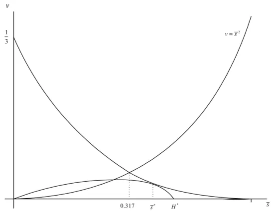
(23) located below the curve v = s2 . In particular, since the positive root of the equation ". Ã. ln(2) 3 tanh 2s. !#−1. − s = s2. is located at s = 0.317186, it turns out that the H minimizing point, s∗ , must satisfy s∗ > 0.317186, as is shown in figure 4. v 1 3. v= s2. 0.317. s*. H*. s. Figure 4: H(v ∗ (s∗ ), s∗ ) ≤ H(v ∗ (s), s), for all s : 0 ≤ s ≤ 1 Directly from this, we can state: Theorem 11 Assuming an industrial configuration that maximizes social welfare with a discrete number of firms, the one that minimizes the value of H can only 23.

(24) correspond to either 2 or 3 firms in total.. Proof. Since the industrial configuration of a discrete number for n can only correspond to a value of the average market share that is selected from the series n. o. s = 1, 12 , 13 , 14 , ... , it is clear from figure 4 that 1 > s∗ > 14 . Hence it can only be that s∗ is either. 1 2. or 13 .. Naturally, theorem 11 stands in contrast with the point on v ∗ (s) that maximizes social welfare, which, since social welfare on v∗ (s) is given by 2z , is clearly where z → ∞, that is, s → 0. 4. A viable alternative. Since the H index is not really a very good proxy for social welfare, we consider in this section if there exists any other measure that is better, and that only uses the same information as H, namely the vector of market shares. The answer is, of course, affirmative, although we must assume that the market in question functions according to quantity competition with constant and common marginal costs and linear demand. In fact, we shall see that we require far less information than the entire market share vector. Given the assumption of quantity competition, constant common marginal costs and linear demand, the Generalized Stackelberg model discussed above will correctly describe all possible situations. Here, we can even discard the assumption that the 24.

(25) market works with an industrial configuration that is optimal from a social welfare point of view, that is, we now allow for a general number of firms at each level. As was mentioned above, the vector of market shares that correspond to such a situation is given by (11). In particular, note that 1 s∗z = f M (n, z) − 1. that is, social welfare can be written as only a function of the market share of each of the firms at the lowest level f(s) = M. 1 + s∗z s∗z. (14). Given this, we can directly state:. Theorem 12 Any merger, between any number of firms at any levels, that has the final effect of increasing (decreasing) the equilibrium market share of the firms at the final level will have the effect of decreasing (increasing) social welfare.. Proof. The proof is immediate, since the derivative of (14) is f 1 ∂M =− ∗ 2 >0 ∗ ∂sz (sz ). The rule implied by Theorem 12 is particularly simple, easy to use, and covers any particular merger (not only mergers that directly affect the firms at level z). Indeed, 25.

(26) it will also work when, instead of mergers, firms are created and inserted at any level of the hierarchy. However, the rule is certainly not intuative, since it states that a merger will increase social welfare if it results in a lower market share for each of the smallest firms. This goes against traditional anti-trust ideas that mergers that reduce the market shares of small firms should be opposed.. 5. Conclusions. In this paper we have considered the appropriablity of the Herfindahl-Hirshman index as a basis for anti-trust policy regarding mergers in oligopoly markets. We firstly introduced two graphical interpretations of the index, and used them to show how the index can be affected by mergers that reduce the total number of firms active. We have also showed that the H index will never be minimized in the social welfare maximizing industrial configuration of a market with a given total number of firms, in which there is quantity competition, constant and common marginal costs and linear demand. Furthermore, assuming a social welfare maximizing industrial configuration, the H index is minimized for a smaller total number of firms than what would be desireable from a social welfare point of view. Given the obvious problems that the use of the H index implies, we have suggested a second measure that does indeed correctly identify merger activity that is social welfare enhancing, and that does not require any more information than the H index. 26.

(27) (indeed, it requires far less). The suggested measure is simply the market share of the smallest firms that are active; if a merger causes the market share of the smallest firms to fall, then it will increase social welfare.. References Anderson, S. y M. Engers (1992). “Stackelberg versus Cournot Oligopoly Equilibrium”. International Journal of Industrial Organization. 10, 127-135. Deneckere, R, y C. Davidson (1985), “Incentives to Form Coalitions with Bertrand Competition”. RAND Journal of Economics. 16, 473-86. Economides, N. (1993). “Quantity Leadership and Social Inefficiency”. International Journal of Industrial Organization. 11, 219-237. Farrell, J. y C. Shapiro (1990), “Horizontal Mergers: An Equilibrium Analysis”. American Economic Review. 80, 107-26. Fisher, F. (1987), “Horizontal Mergers: Triage and Treatment”. Journal of Economic Perspectives. 1, 2, 23-40. Hamilton, J. and S. Slutsky. (1990). “Endogenous Timing in Duopoly Games: Stackelberg or Cournot Equibliria”. Games and Economic Behavior. 2, 29-46.. 27.

(28) Kamien, M. y I. Zang (1990), “The Limits of Monopolization Through Acquisition”. Quarterly Journal of Economics. 2, 465-499. Levin, D. (1990). “Horizontal Mergers: The 50% Benchmark”. American Economic Review. 80, 1238-1245. Matsumura, T. (1999). “Quantity-setting Oligopoly with Endogenous Sequencing”. International Journal of Industrial Organization. 17, 289-296. Salant, S., S. Switzer y R. Reynolds (1983), “Losses From Horizontal Merger: The Effects of an Exogenous Change in Industry Structure on Cournot-Nash Equilibrium”. Quarterly Journal of Economics. XCVIII, 185-199. Salop, S. (1987), “Symposium on Mergers and Antitrust”. Journal of Economic Perspectives. 1, 2, 3-12. Schmalensee, R. (1987), “Horizontal Merger Policy: Problems and Changes”. Journal of Economic Perspectives. 1, 2, 41-54. Sherali, H. (1984), “A Multiple Leader Stackelberg Model and Analysis”. Operations Research. 32, 390-404. Watt, R. (2002), “A Generalized Oligopoly Model”, Metroeconomica. 53(1), 46-55.. 28.

(29) White, L. (1987), “Antitrust and Merger Policy: A Review and Critique”. Journal of Economic Perspectives. 1, 2, 13-22.. 29.

(30)