TítuloNovel parallelization of simulated annealing and Hooke & Jeeves search algorithms for multicore systems with application to complex fisheries stock assessment models
13
0
0
Texto completo
(2) mal search procedure for a specific task [e.g. 3, 4], but these investigations indicate that a particular combination is problem specific. Various tools have been developed to aid in the creation of statistical stock assessment models. One such tool is Gadget (Globally applicable Area Disaggregated General Ecosystem Toolbox), which is a modeling environment designed to build models for marine ecosystems, including both the impact of the interactions between species and the impact of fisheries harvesting the species [5, 6]. It is an open source program written in C++ and it is freely available from the Gadget development repository at www.github.com/hafro/gadget. Gadget works by running an internal model based on many parameters describing the ecosystem, and then comparing the output from this model to observed measurements to obtain a goodness-of-fit likelihood score. By using one or several search algorithms it is possible to find a set of parameter values that gives the lowest likelihood score, and thus better describe the modeled ecosystem. The optimization process is the most computationally intensive part of the process as it commonly involves repeated evaluations of the computationally expensive likelihood function, as the function calls a full ecosystem simulation for comparison to data. In addition to that, multiple optimization cycles are sometimes performed to ensure that the model has converged to an optimum as well as to provide opportunities to escape from a local minimum, using heuristics such as those described by [7]. Once the parameters have been estimated, one can use the model to make predictions on the future evolution of fish stocks. Gadget can be used to assess a single fish stock or to build complex multi-species models. It has been applied in many ecosystems such as the Icelandic continental shelf area for the cod and redfish stocks [7, 8, 9], the Bay of Biscay in Spain to predict the evolution of the anchovy stock [10], the North East Atlantic to model the porbeagle shark stock [11], or the Barents Sea to model dynamic species interactions [12]. Models developed using the Gadget framework have also been used to provide tactical advice on sustainable exploitation levels of a particular resource. Notably the southern European Hake stock,. Icelandic Golden redfish, Tusk and Ling stocks, and Barent sea Greenland halibut are formally assessed by the International Council for the Exploration of the Sea (ICES) using Gadget [see 13, 14, 15, 16, for further details]. The aim of this work is to speedup the costly optimization process of Gadget so that more optimization cycles can be performed and a more reliable model can be achieved. The methodology followed comprises three main stages: First, the code was profiled in order to identify its bottlenecks; then, sequential optimizations were applied to reduce these bottlenecks; finally, the most used optimization algorithms were parallelized. Currently, there are three different optimization algorithms implemented in Gadget: the Simulated Annealing (SA) algorithm [17], the Hooke & Jeeves (H&J) algorithm [18], and the Broyden-FletcherGoldfarb-Shanno (BFGS) algorithm [19]. All of them can be used alone or combined into a single hybrid algorithm. Combining the wide-area searching characteristics of SA with the fast local convergence of H&J is, in general, an effective approach to find an optimum solution. In this work both algorithms have been parallelized using OpenMP [20], so that the proposed solution can take advantage of today’s ubiquitous multicore systems. The rest of this paper is organized as follows. Section 2 covers related work. Section 3 describes the sequential optimizations applied. Sections 4 and 5 describe the basics of the SA and the H&J search algorithms and discuss the parallelization strategies proposed for each one of them. Section 6 presents the experimental evaluation of all the proposals on a multicore system. Finally, conclusions are discussed in Section 7. 2. Related Work There exist in the literature a large number of solutions for the parallel implementation of the SA algorithm on distributed memory systems [21, 22, 23, 24, 25] In [24] five different parallel versions are implemented and compared. The main difference among them is the number of communications required and the quality of the solution. The solution is better 2.
(3) when the communication among the processes increases. However, in distributed memory systems the communication overhead plays a important role in the global performance of the parallel algorithm. Thus, solutions where communication takes place after every move are not considered a good alternative on these architectures. In shared-memory systems, however, this kind of solution is viable in terms of computational efficiency, as in this case the communications are performed through the use of shared variables. Parallelization proposals for shared-memory systems are much more scarce. In [26] A. Bevilacqua implements an adaptive parallel algorithm for a nondedicated shared memory machine using the POSIX Pthreads [27] library. The program execution flow switches dynamically at run-time between the sequential and the parallel algorithm depending on the acceptance ratio and the workload conditions of the machine. Paramin [28, 6] is a parallel version of Gadget originally written with PVM [29], and later migrated to MPI [30]. As the parallel version proposed in this paper, Paramin is based on the distribution of the function evaluations among the different processes. However, unlike our approach, in each parallel step it updates all the parameters whose moves lead to a better likelihood value. Moves that are beneficial one by one could become counterproductive when they are applied together. Thus, this parallel version leads to a worse likelihood score in some cases, an important problem that does not happen in our version. Additionally, Paramin is meant to be executed in a distributed infrastructure, such as a cluster of computers, and it needs an installed version of the MPI library. On the other hand, our approach focuses on taking advantage of common desktop multicore systems and it only needs to add the appropriate OpenMP compile-time flag to the selected compiler, reducing the computing expertise needed to profit from it.. First, some light class member functions that were invoked very often in the application from other classes could not be inlined by the compiler because they were not expressed in the header files that describe their associated classes, but in the associated implementation files. Moving their definition to the header file allowed their effective inlining, largely reducing their weight in the runtime. Second, we found several opportunities to avoid recalculations of values, i.e., computations that are performed several times on the same inputs, thus yielding the same result. While some of these opportunities could be exploited just by performing loopinvariant code motion, other more complex situations required a more elaborated approach such as dynamically building tables to cache the results of these calculations and later resorting to these tables to get the associated results. The third most important optimization applied consisted in modifying the data structure used to represent bidimensional matrices in the heaviest functions. The original code used a layout based on an array of pointers, each pointer allowing the access to a row of the matrix that had been separately allocated. These matrices were changed to be stored using a single consecutive buffer, thus improving the locality, avoiding indirections and helping the compiler to reason better on the code. 4. Parallelization of the Simulated Annealing Algorithm. The SA algorithm used in Gadget is a global optimization method that tries to find the global optimum of a function of N parameters. At the beginning of each iteration, this search algorithm decides which parameter np it is going to be modified to explore the search space. Then, the algorithm generates a trial point with a value of this parameter that is within the step length given by element np −−→ of vector V M (of length N) of the user selected starting point by applying a random move. The function is evaluated at this trial point and its result 3. Optimization of the Sequential Program is compared to its value at the initial point. When The profiling of the original application revealed minimizing a function, any downhill step is accepted that it could be optimized mainly in three aspects. and the process repeats from this new point. An 3.
(4) 1. 2 3 4 5 6 7 8 9 10 11 12 13 14 15 16 17 18 19 20 21 22 23 24 25. −−→ → Algorithm SimulatedAnnealing(− p , V M , ns, T, nt, M axIterations) → input : - initial vector of N parameters − p = pi , 1 ≤ i ≤ N −−→ - step lengths vector with one element per parameter V M = V Mi , 1 ≤ i ≤ N −−→ - frequency of V M updates ns - temperature T - frequency of temperature T reductions nt - maximum number of evaluations M axIterations → output: optimized vector of N parameters − p = pi , 1 ≤ i ≤ N iterations = 0 parami = i, 1 ≤ i ≤ N //permutation of parameters → bestLikelihood = evaluate(− p) → while not terminationTest(bestLikelihood, − p ) do for a = 1 to nt do −−−→ reorder(− param) for j = 1 to ns do for i = 1 to N do iterations = iterations + 1 np = parami //parameter to modify − −−−→ = − → tmp_p p −−→ tmp_pnp = adjustParam(pnp , V M ) − − − − → likelihood = evaluate(tmp_p) −−−→ → accept(T, bestLikelihood, likelihood, − p ,− tmp_p) if iterations = M axIterations then → return − p end end end −−→ adjustVM(V M ) end reduceTemperature(T ) end → return − p. Figure 1: Simulated Annealing algorithm. −−→ that direction. Also, each nt adjustments to V M the temperature is reduced. Thus, a temperature reduction occurs every ns × nt cycles of moves along every direction (each ns × nt × N evaluations of the function). When T declines, uphill moves are less likely to be accepted and the percentage of rejections −−→ rises. Given the scheme for the selection for V M , −−→ −−→ V M falls. Thus, as T declines, V M falls and the algorithm focuses upon the most promising area for optimization. The process stops when no more improvement can be expected or when the maximum number of function evaluations is reached. A pseudocode of the SA algorithm is shown in Figure 1.. uphill step may be also accepted to escape from local minimum. This decision is made by the Metropolis criteria. It uses a variable called Temperature (T) and the size of the uphill move in a probabilistic manner to decide the acceptance. The bigger T and the size of the uphill move are, the more likely that move will be accepted. If the trial is accepted, the algorithm moves on from that point. If it is rejected, another point is chosen instead for a trial evaluation. Each ns evaluations of the N parameters −−→ the elements of V M are adjusted so that half of all function evaluations in each direction will be accepted. Thus, the modification of each element of −−→ V M depends on the number of moves accepted along. 4.
(5) This algorithm was parallelized using OpenMP. The followed parallelization pattern consisted in subdividing the search process in a number of steps that are applied in sequence, parallelism being exploited within each step. Since the expensive part of a search algorithm is the evaluation of the fitness function, the parallelism is exploited by distributing the function evaluations across the available threads. The results of the evaluations are stored in shared variables so that all the values can be analyzed by the search algorithm in order to decide whether to finish the search process, and if this is not the case, how to perform the next search step. This work aims to reduce the execution time without diminishing the quality of the solution. For this purpose, two parallel algorithms were developed: the reproducible and the speculative algorithm. The first one follows exactly the same sequence as the original serial algorithm, and thus it finishes in the same point and with the same likelihood score. The speculative version, however, is allowed to change the parameter modification sequence in order to increase the parallelism, and thus it can finish in a different point and with a different likelihood value. In this latter case, some specification variables of the sequential algorithm were adapted to prevent the algorithm from converging to a worse likelihood value. In the parallel versions not all the functions evaluations provide useful information to the search process. Thus, the number of effective evaluations is taken into account as ending criterion instead of the number of total evaluations. The same parallelization strategies have been applied to the H&J algorithm, described in Section 5.. From these evaluations the algorithm moves to the first point (in sequential order) that is accepted (directly or applying the Metropolis criteria), dismissing the others. As a result, all the evaluations up to the first one with an accepted point are taken into account to advance in the search process, and for this reason they will be counted as effective evaluations, while all the subsequent simulations are discarded. For the previous example, if the modification to the first parameter is rejected and the modification to the second parameter is accepted, the calculations performed by threads 1 and 2 are considered, and the calculations by threads 3 and 4 are discarded, even if one of them obtains a better likelihood that the obtained by thread 2. In this case, 4 evaluations are performed in parallel but only 2 of them are recorded as effective evaluations. Following our example, since the last evaluation considered modified the second parameter, in the next step, thread 1 will perform the evaluation modifying the third parameter, thread 2 the fourth parameter, thread 3 the fifth parameter, and thread 4 the sixth parameter. In order to obtain the same result as in the sequential algorithm, the parameters re-evaluated will take the same value as in the previous step. This required changing the way of generating the random values. Namely, while the sequential version relies on rand, the reproducible version uses a random function which generates its result from a seed provided by the user. This allows to re-generate previously generated random values by providing the same seed, which is recorded by our implementation for this purpose. Another change was that while the random numbers of the sequential version follow a single sequence, the parallel version uses three different seeds, giving place to three sequences of ran4.1. Reproducible version dom numbers. One seed (seedP) is used to change In this version each thread performs the eval- the order in which the parameters are modified, anuation of the function with the modification of a other one (seedM) is used for the acceptance of the different parameter in parallel. For example, with Metropolis criteria, and the last one (seed) is used four threads, in the first step, the thread 1 could for the calculation of the new value of the parameters. perform the evaluation changing the first parameter, the thread 2 the second parameter, the thread 3 4.2. Speculative version the third parameter, and the thread 4 the fourth As in the reproducible version, each thread parameter. performs the evaluation with the modification of a different parameter in parallel, but now the move 5.
(6) with the best likelihood is selected. This point improves the likelihood, or (b) the change in that will be accepted if it obtains a better likelihood parameter does not improve the likelihood but it than the initial point. Otherwise, the Metropolis happens to be the best one and it is accepted apcriteria is applied to decide its acceptance. For plying the Metropolis criteria. Notice that the example, with 4 threads, in the first step thread second situation implies that none of the changes 1 could perform the simulation changing the first improved the likelihood. parameter, thread 2 the second parameter, thread 3 the third parameter and thread 4 the fourth ns: In the parallel algorithm not all the parameter modifications provide useful information to the parameter. If thread 3 obtains the best likelihood, search process. Thus, to avoid to change the the modification of the third parameter will be −−→ step lenght associated to each parameter (V M the one accepted and the other modifications will vector) too often, in addition to the global scalar be discarded. In the next parallel step, thread 1 −→ has been defined with the aim ns, a vector − vns will work with a change in the fifth parameter, of processing the step length individually. It is thread 2 in the sixth parameter, thread 3 in the sevincreased whenever (a) the change simulated in enth parameter and thread 4 in the eighth parameter. the parameter improves the likelihood, or (b) the parameter change is rejected (also applying the Note that the speculative version performs and Metropolis criteria). This way, it is increased in considers evaluations that are never performed in all the situations except when the change would the sequential version. This makes it follow search be accepted by the Metropolis criteria. paths that are different from those of the sequential and the reproducible versions. For this reason, this algorithm can finish in a different point and with a different likelihood value.. Also, in order to avoid decreasing the temperature too fast, which would lead to a premature halt of the algorithm, it is necessary to take into account that the number of discarded evaluations increases with the number of threads used in the parallel algorithm. For this reason now each temperature iteration consists of ns × numT hreads/2 parallel steps, that is, ns×numT hreads/2×numT hreads evaluations, where ns is the scalar with the same value as in the sequential version and numT hreads is the number of threads used to execute the parallel version.. In this version, unlike in the reproducible version, some discarded simulations provide information to the search process even though they do not modify the parameters. This forced us to adapt some of the most important variables used during the search process. These variables, which we describe providing their semantics in the sequential version, are: − −→ vector that stores for each parameter the numnacp:. ber of times a change in its value has been accepted. It affects the calculation of the step Finally, the counter of the number of effective eval−−→ lengths vector V M , explained at the beginning uations increases every time a parameter change is −→ the larger of Section 4. Namely, the higher − nacp, rejected (also applying the Metropolis criteria) and −−→ value will have V M and the changes performed once for every parallel step. in the parameter will be bigger. ns: scalar that provides the frequency of updates to −−→ V M.. 5. Parallelization of the Hooke & Jeeves Algorithm. For this parallel version the above variables were Hooke and Jeeves (H&J) [18] is a pattern search changed as follows: method that consists in a sequence of exploratory − −→ Its value for a given parameter increases when- moves from a base point, followed by pattern moves nacp: ever (a) the change evaluated in that parameter that provide the next base point to explore. 6.
(7) 1. 2 3 4 5 6 7 8 9 10 11 12 13 14 15 16 17 18 19 20 21 22 23 24 25 26. −−−→ → Algorithm HookeJeeves(− p , delta, M axIterations, rho) → input : - initial vector of N parameters − p = pi , 1 ≤ i ≤ N −−−→ - modification length for each parameter delta = deltai , 1 ≤ i ≤ N - maximum number of evaluations M axIterations - reduction control variable rho → output: optimized vector of N parameters − p = pi , 1 ≤ i ≤ N iterations = 0 − −−−→ = − → tmp_p p → bestLikelihood = evaluate(− p) initialLikelihood = bestLikelihood → while not terminationTest(iterations, M axIterations, bestLikelihood, − p ) do iterations = iterations + 1 for i = 1 to N do tmp_pi = pi + deltai −−−→ likelihood = evaluate(− tmp_p) if likelihood < bestLikelihood then bestLikelihood = likelihood else tmp_pi = pi − deltai −−−→ likelihood = evaluate(− tmp_p) if likelihood < bestLikelihood then bestLikelihood = likelihood else tmp_pi = pi end end end −−→ −−−→ − → adjust(− p, − tmp_p, delta, rho, initialLikelihood, bestLikelihood) //includes exploratory moves − − − − → − → p = tmp_p end → return − p. Figure 2: Hooke & Jeeves algorithm. The exploratory stage performs local searches in each direction by changing a single parameter of the base point in each move. For each parameter, the algorithm considers first an increment delta in the positive direction. If the function value in this point is better than the old one, then the algorithm selects this new point like the new base point. Otherwise, an increase delta is done in the negative direction, and if the result is better than the original one, then the algorithm selects this new point as the base point. Otherwise the algorithm keeps the initial value and proceeds to evaluate changes in the next parameter. Once all the parameters have been explored, the algorithm continues with the pattern moves stage.. In the pattern stage, each one of the parameters is increased by an amount equal to the difference between the present parameter value and the previous one (its value before the exploratory stage). The aim is to move the base point towards the direction that improved the result during the previous stage. Then, the function is evaluated in this new point. If the function value is better, this point becomes the new base point for the next exploratory moves. Otherwise, the pattern moves are ignored. The search proceeds in series of these two stages until a minimum is found or the maximum number of evaluations is reached. If after a exploratory stage the base point does not change, delta is reduced. The amount of the reduction is determined by a user7.
(8) supplied parameter called rho. Taking big steps gets to the minimum more quickly, at the risk of stepping right over an excellent point. Figure 2 summarizes this search algorithm. The parallel implementations of this algorithm use nested parallelism to parallelize the exploratory stage. At the top level, each thread is in charge of evaluating the changes on a specific parameter. Then, each thread is split in two threads, so that one of them evaluates the movement in the positive direction and the other one the movement in the negative direction. For this reason, the required number of threads to execute these versions is a multiple of 2. For example, if we have 4 threads, in the first parallel evaluation one thread will evaluate parameter 1 + delta, another one the parameter 1 - delta, another one the parameter 2 + delta and finally another one the parameter 2 - delta.. starts the evaluations of the next parallel step from parameter n + 1. For this version the counter of the number of effective evaluations is only increased in two situations. First, for every parameter in which none of the movements improved the likelihood, the counter is increased by two units, to account for the two movements tested. Second, among all those movements that improve the likelihood, only the best one in the parallel step is considered. If this movement is in the positive direction, the counter is increased by one unit, otherwise it is increased by two units, because negative movements are always evaluated after a positive movement has been discarded.. Finally, the outer loop that iterates on the parameters to perform the exploratory moves has step numT hreads/2, since each parallel step evaluates the two possible movements for numT hreads/2 5.1. Reproducible version The reproducible version follows exactly the same parameters. sequence as the original sequential algorithm. This version chooses the first move (in sequential order) that improves the likelihood as base point for the next search step. All the subsequent evaluations are 6. Experimental Results disregarded and they will not be taken into account The different parallel implementations were evaluto increase the counter of the number of effective evalated in an HP ProLiant XL230a Gen9 server running uations. For the previous example using 4 threads, if the the Scientific Linux release 6.4. It consists of two first evaluation that obtains a better likelihood processors Intel Haswell E5-2680 at 2.5 GHZ with 12 corresponds to the movement of the first parameter cores per processor and 64 GB of memory. All the in the negative direction (parameter 1 - delta), codes were compiled with the gnu g++ compiler verthe two evaluations using the second parameter sion 4.9.1 and the compilation flag -O3. Three differare discarded (parameter 2 + delta and parameter ent models were used to better evaluate the results: 2-delta). The next step will start from parameter 2 and it will evaluate the moves in the positive and IEO: This model is used by the IEO to assess the southern hake stock. It counts with 63 paramenegative direction of both parameters 2 and 3. ters to optimize. TUSK: It is a single-species model of tusk (brosme brosme) in Icelandic waters which is used by This version chooses the move that gives place to ICES as the basis for catch advice. It counts the best likelihood as base point for the next search with 48 parameters to optimize. step. Since all the evaluations are taken into account to choose this value, if n was the last parameter HADOCK: It is a single-species, single-area model considered in a parallel step, this version always used to model the Icelandic haddock. It is the 5.2. Speculative version. 8.
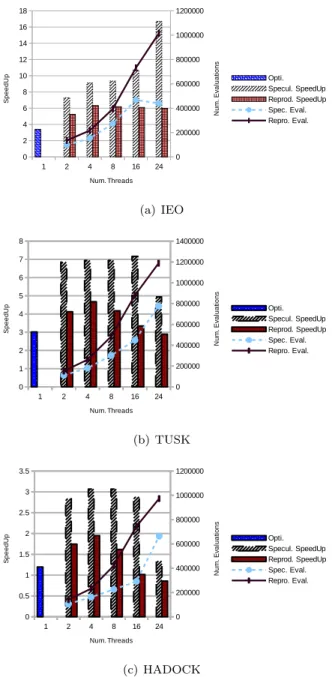
(9) IEO TUSK HADOCK. SA 5264 4699 1178. H&J 5266 4741 1177. SA + H&J 10504 9372 2362. Table 1: Execution times, in seconds, of the original code using a single search algorithm or both. example model provided with Gadget. It is available for download from the Gadget website. It counts with 38 parameters to optimize. (a) IEO. The performance of the parallel algorithms was evaluated in terms of both the computational efficiency (speedup) and the quality of the solutions (likelihood score obtained). All the speedups were calculated with respect to the execution time of the original sequential application (Gadget v2.2.00, available at www.hafro.is/gadget/files/gadget2.2.00.tar.gz). These execution times are shown in Table 1, and they correspond to the whole execution of the application, either using a single search algorithm or two. In all the experiments the optimization algorithms stop when the maximum number of effective evaluations (1000 for both algorithms) is reached. Figure 3 shows the speedups for the optimized sequential version and the two parallel versions developed, the reproducible one and the speculative one, when using only the SA algorithm, for the 3 model examples considered and for different number of threads. The total number of evaluations performed for the parallel algorithms is also shown in the figures. The optimization of the sequential code obtains a significant reduction in the execution time, achieving a speedup of 3.3 for the IEO model. As regards the parallel versions, the number of performed evaluations increases with the number of threads, being this increment larger for the reproducible version, as a greater number of evaluations has to be discarded in this case. For this reason, the speedup of the reproducible version does not improve beyond 4 cores. The speculative version behaves better, although the results depend significantly on the example model. The best results are for the IEO model because in this case. (b) TUSK. (c) HADOCK Figure 3: Speedups using the SA algorithm, fill bars indicate relative speedup and the lines the number of function calls as a function of number of threads and by approach.. the starting point is closer to the optimum point (see Table 2, discussed at the end of this section), which increases the rate of rejects and thus, the number of 9.
(10) effective evaluations. Note that for this example the number of total evaluations does not increase as fast as in the other models.. (a) IEO. (a) IEO. (b) TUSK. (b) TUSK. (c) HADOCK Figure 5: Speedups using the SA and the H&J algorithms, fill bars indicate relative speedup and the lines the number of function calls as a function of number of threads and by approach.. (c) HADOCK Figure 4: Speedups using the H&J algorithm, fill bars indicate relative speedup and the lines the number of function calls as a function of number of threads and by approach.. Similar results are obtained for the H&J algorithm, as can be seen in Figure 4. Finally, Figure 5 shows 10.
(11) Initial Sequential 2 4 8 16 24. IEO 1015.1691 1015.1130 1015.1120 1014.8995 1015.0495 1015.0250 1015.0400. TUSK 26128.3060 6537.8195 6539.2886 6511.2774 6509.1936 6507.5369 6507.1087. HADOCK 0.96417375 0.85868597 0.86255539 0.85186922 0.85107118 0.85250038 0.85083064. Initial Sequential 2 4 8 16 24. Table 2: Likelihood obtained using SA. IEO 1015.1691 1015.0780 1015.0780 1015.1062 1015.1045 1015.1081 1015.0817. TUSK 26128.3060 6837.3983 6837.3983 6953.9042 6891.2857 6898.9408 6963.9621. HADOCK 0.96417375 0.87042278 0.87042278 0.85509464 0.86385086 0.86559744 0.86008887. Table 3: Likelihood obtained using H&J. Initial Sequential 2 4 8 16 24. IEO 1015.1691 1015.0478 1015.0641 1014.8474 1014.9955 1014.9662 1014.9820. TUSK 26128.3060 6511.6363 6515.1060 6508.4827 6507.3761 6507.0652 6507.0435. HADOCK 0.96417375 0.85396624 0.85601157 0.85074075 0.85070340 0.85150650 0.85058013. the speedups when using the SA and the H&J algorithms in sequence. This hybrid algorithm combines the power and robustness of the SA algorithm with the faster convergence of a local method as the H&J algorithm. It is a common choice as, in general, it is an effective approach to find an optimum point. Note that the speedup of the reproducible version only imTable 4: Likelihood obtained using SA & H&J proves up to 4 cores, whereas the speculative version obtains the best results when using 16 or 24 cores. The best results are for the IEO model, where the 7. Conclusions execution time is reduced from 175 to 23 minutes using the reproducible version and 4 cores and to only The aim of this work has been to speedup the Gad12 minutes using the speculative version and 24 cores. get program to reach a reliable model in a reasonable execution time, getting profit from the new multiAs regards the quality of the solution, the repro- core architectures. First, the sequential code was anducible versions obtain exactly the same likelihood alyzed and optimized so that the most important botscore as the original sequential version. The scores tlenecks were identified and reduced. Then, the SA for the speculative version for SA, H&J and the hy- and H&J algorithms, used to optimize the model probrid SA-H&J algorithms are shown in Tables 2, 3 and vided by Gadget, were parallelized using OpenMP. 4, respectively. The tables also show for comparative Two different versions were implemented for each alpurposes the starting likelihood value associated to gorithm, the speculative one, which yields the same the input (Initial row in the tables) and the value af- result as the sequential version, and the speculative ter applying the sequential optimization algorithms version, which can exploit more parallelism. It must (Sequential row). Notice that the likelihood value is be stressed that all the parallel algorithms proposed better the lower it is, thus the search algorithms re- are totally general and can thus be applied to other duce it. We can see that some models, like IEO, be- optimization problems. As expected, the speculative gin with values near the optimum point found, while version provides better results for all the analyzed exothers, such as TUSK, can be strongly optimized by amples, achieving a speedup of 14.8 (4.5 with respect Gadget. As expected, the best likelihood value is to the optimized sequential version) for the hybrid obtained with the hybrid algorithm and this value SA-H&J algorithm and the IEO model on a 24-core is even improved when using the parallel speculative server. Moreover, the speculative version not only version. reduces significantly the execution time, but it also 11.
(12) obtains a better likelihood score. OpenMP is nowadays the standard de facto for shared memory parallel programming and it allows the efficient use of today’s mainstream multicore processors. The OpenMP versions of the Gadget software developed in this work will allow researchers to make a better use of their computer resources. They are publicly available under GPLv2 license at www.github.com/hafro/gadget. Acknowledgment This work has been partially funded by the Galician Government (Xunta de Galicia) and FEDER funds of the EU under the Consolidation Program of Competitive Research Units (Network ref. R2014/041) and by European Union’s Seventh Framework Programme for research, technological development and demonstration under grant agreement no.613571. Authors gratefully thank CESGA (Galicia Supercomputing Center, Santiago de Compostela, Spain) for providing access to the HP ProLiant XL230a Gen9 server and Santiago Cerviño from IEO for his support.. [5] J. Begley, D. Howell, An overview of Gadget, the globally applicable area-disaggregated general ecosystem toolbox, ICES, 2004. [6] J. Begley, Gadget user guide, http://www. hafro.is/gadget/files/userguide.pdf (2012). [7] L. Taylor, J. Begley, V. Kupca, G. Stefansson, A simple implementation of the statistical modelling framework Gadget for cod in Icelandic waters, African Journal of Marine Science 29 (2) (2007) 223–245. [8] H. Björnsson, T. Sigurdsson, Assessment of golden redfish (sebastes marinus l) in icelandic waters, Scientia Marina 67 (S1) (2003) 301–314. [9] B. Elvarsson, L. Taylor, V. Trenkel, V. Kupca, G. Stefansson, A bootstrap method for estimating bias and variance in statistical fisheries modelling frameworks using highly disparate datasets, African Journal of Marine Science 36 (1) (2014) 99–110.. [10] E. Andonegi, J. A. Fernandes, I. Quincoces, X. Irigoien, A. Uriarte, A. Pérez, D. Howell, References G. Stefánsson, The potential use of a Gadget model to predict stock responses to climate [1] J. J. Pella, P. K. Tomlinson, A generalized change in combination with bayesian networks: stock production model, Inter-American Tropthe case of Bay of Biscay anchovy, ICES Jourical Tuna Commission, 1969. nal of Marine Science: Journal du Conseil 68 (6) (2011) 1257–1269. [2] K. Patterson, R. Cook, C. Darby, S. Gavaris, L. Kell, P. Lewy, B. Mesnil, A. Punt, V. Restrepo, D. W. Skagen, et al., Estimating uncer- [11] S. McCully, F. Scott, L. Kell, J. Ellis, D. Howell, A novel application of the Gadget operating tainty in fish stock assessment and forecasting, model to North East Atlantic porbeagle, Collect. Fish and Fisheries 2 (2) (2001) 125–157. Vol. Sci. Pap. ICCAT 65 (6) (2010) 2069–2076. [3] G. Einarsson, Competitive coevolution in problem design and metaheuristical parameter tun- [12] D. Howell, B. Bogstad, A combined Gadget/FLR model for management strategy evaling, M.Sc. Thesis. University of Iceland, Iceland uations of the Barents Sea fisheries, ICES Jour(2014)http://hdl.handle.net/1946/18534. nal of Marine Science: Journal du Conseil 67 (9) [4] A. Punt, B. Elvarsson, Improving the perfor(2010) 1998–2004. mance of the algorithm for conditioning implementation simulation trials, with application [13] Report of the working group on the assessto north atlantic fin whales, IWC Document ment of southern shelf stocks of hake, monk and SC/D11/NPM1 (7pp). megrim, Tech. Rep. ICES CM 2010/ACOM:11, 12.
(13) International Council for the Exploration of the [24] E. Onbaşoğlu, L. Özdamar, Parallel simulated Sea (2010). annealing algorithms in global optimization, Journal of Global Optimization 19 (1) (2001) [14] Report of the benchmark workshop on deep27–50. sea stocks (wkdeep), Tech. Rep. ICES CM 2014/ACOM:44, International Council for the [25] D.-J. Chen, C.-Y. Lee, C.-H. Park, P. Mendes, Parallelizing simulated annealing algorithms Exploration of the Sea. based on high-performance computer, Journal of Global Optimization 39 (2) (2007) 261–289. [15] Report of the benchmark workshop on redfish management plan evaluation (wkredmp), Tech. [26] A. Bevilacqua, A methodological approach to Rep. ICES CM 2014/ACOM:52, International parallel simulated annealing on an smp system, Council for the Exploration of the Sea. Journal of Parallel and Distributed Computing 62 (10) (2002) 1548–1570. [16] Report of the inter benchmark process on greenland halibut in ices areas i and ii (ibphali), Tech. [27] D. R. Butenhof, Programming with POSIX Rep. ICES CM 2015/ACOM:54, International Threads, Addison Wesley, 1997. Council for the Exploration of the Sea. [28] G. Stefánsson, A. Jakobsdóttir, B. Elvarsson, [17] A. Corana, M. Marchesi, C. Martini, S. Ridella, J. Begley, Paramin, a composite parallel alMinimizing multimodal functions of continuous gorithm for minimising computationally expenvariables with the ’Simulated Annealing’ alsive functions, http://www.hafro.is/gadget/ gorithm, ACM Transactions on Mathematical files/paramin.pdf (2004). Software (TOMS) 13 (3) (1987) 262–280. [29] A. Geist, PVM: Parallel Virtual Machine: a users’ guide and tutorial for networked parallel [18] R. Hooke, T. A. Jeeves, Direct search solution computing, MIT press, 1994. of numerical and statistical problems, Journal of the ACM (JACM) 8 (2) (1961) 212–229. [30] MPI Forum, Message Passing Interface, http: //www.mpi-forum.org. [19] D. P. Bertsekas, Nonlinear programming, Athena scientific, 1999. [20] OpenMP website, http://openmp.org/. [21] D. R. Greening, Parallel simulated annealing techniques, Physica D: Nonlinear Phenomena 42 (1) (1990) 293–306. [22] E. E. Witte, R. D. Chamberlain, M. Franklin, et al., Parallel simulated annealing using speculative computation, Parallel and Distributed Systems, IEEE Transactions on 2 (4) (1991) 483–494. [23] D. J. Ram, T. Sreenivas, K. G. Subramaniam, Parallel simulated annealing algorithms, Journal of parallel and distributed computing 37 (2) (1996) 207–212. 13.
(14)
Figure


+2

Documento similar
Results obtained with the synthesis of the operating procedure for the minimize of the startup time for a drum boiler using the tabu search algorithm,
For this work we have implemented three algorithms: algorithm A, for the estimation of the global alignment with k differences, based on dynamic programming; algorithm B, for
Government policy varies between nations and this guidance sets out the need for balanced decision-making about ways of working, and the ongoing safety considerations
No obstante, como esta enfermedad afecta a cada persona de manera diferente, no todas las opciones de cuidado y tratamiento pueden ser apropiadas para cada individuo.. La forma
To verify the nonlinear model, a simplified version for small oscillations is obtained and compared with other results [12-14] using reduced linear models for the triple
- Competition for water and land for non-food supply - Very high energy input agriculture is not replicable - High rates of losses and waste of food. - Environmental implications
In the previous sections we have shown how astronomical alignments and solar hierophanies – with a common interest in the solstices − were substantiated in the
attitudes with respect to the price they pay and would be willing to pay for irrigation water, as well as the marginal product value of the water they use and the potential for
