Predicting soil bulk density using hierarchical pedrotransfer functions and artificial neural networks

Texto completo

(1)PONTIFICIA UNIVERSIDAD CATOLICA DE CHILE ESCUELA DE INGENIERIA. PREDICTING SOIL BULK DENSITY USING HIERARCHICAL PEDOTRANSFER FUNCTIONS AND ARTIFICIAL NEURAL NETWORKS. JORGE SEBASTIÁN SILVA ORELLANA. Thesis submitted to the Office of Research and Graduate Studies in partial fulfillment of the requirements for the Degree of Master of Science in Engineering Advisor: CARLOS BONILLA MELÉNDEZ. Santiago de Chile, April, 2017  MMXVII, Jorge Sebastián Silva Orellana.

(2) PONTIFICIA UNIVERSIDAD CATOLICA DE CHILE ESCUELA DE INGENIERIA. PREDICTING SOIL BULK DENSITY USING HIERARCHICAL PEDOTRANSFER FUNCTIONS AND ARTIFICIAL NEURAL NETWORKS. JORGE SEBASTIÁN SILVA ORELLANA. Members of the Committee: CARLOS BONILLA MELÉNDEZ FRANCISCO SUÁREZ POCH FELIPE ABURTO GUERRERO CÉSAR SÁEZ NAVARRETE. Thesis submitted to the Office of Research and Graduate Studies in partial fulfillment of the requirements for the Degree of Master of Science in Engineering Santiago de Chile, April, 2017.

(3) To my family: parents, grandparents, wife. and. daughter. unconditional support.. ii. for. their.

(4) ACKNOWLEDGEMENTS. First I want to thank my family who supported me all this time. This includes my parents Cecilia Orellana and Enrique Silva, grandparents Jorge Orellana and Cecilia Alfaro, wife Antonieta Ortiz-Arrieta and daughter Marina Silva. I express my greatest gratitude to the advising of Professor Carlos Bonilla for his deep empathy, which leaves me a profound life teaching. Without their guidance, support and patience this study would not have been possible. I would also like to thank to the members of the research team of Professor Bonilla, because of their suggestions and collaboration help me to grow as a researcher. This research was partially supported with funds from the National Commission for Scientific and Technological Research CONICYT/FONDECYT/Regular 1161045. The Vice Rectory of Research scholarship – Pontificia Universidad Católica de Chile is also acknowledged.. iii.

(5) GENERAL INDEX. ACKNOWLEDGEMENTS ........................................................................................ iii LIST OF TABLES ....................................................................................................... v LIST OF FIGURES .................................................................................................... vi RESUMEN................................................................................................................. vii ABSTRACT .............................................................................................................. viii 1.. INTRODUCTION .............................................................................................. 1 1.1. Overwiew ................................................................................................... 1 1.2. Hypothesis .................................................................................................. 4 1.3. Objective .................................................................................................... 5 1.4. Methodology .............................................................................................. 5 1.5. Results ........................................................................................................ 6 1.6. Conclusions ................................................................................................ 6. 2.. LITERATURE REVIEW ................................................................................... 8. 3.. MATERIALS AND METHODS ..................................................................... 11 3.1. Soil samples ............................................................................................. 11 3.2. Artificial neural networks ........................................................................ 15 3.3. Equations tested for predicting soil bulk density ..................................... 16 3.4. Statistical analysis .................................................................................... 20. 4.. RESULTS AND DISCUSSION ....................................................................... 21 4.1. Soil properties in the soil data set ............................................................ 21 4.2. Artificial neural networks ........................................................................ 23 4.3. Evaluation of the previous PTFs .............................................................. 30 4.4. Comparison between the ANN and the calibrated PTFs ......................... 35. 5.. CONCLUSIONS .............................................................................................. 36. REFERENCES........................................................................................................... 37.

(6) LIST OF TABLES. Table 1. Summary of properties of the soil samples used in the study. ........................... 13 Table 2. Pedotransfer functions evaluated in the study. Sample sizes (n), mean ρb and r2 values from the original publications. .............................................................................. 18 Table 3. Correlation matrix (with the Pearson coefficient) between soil properties of Table 1 for the entire soil sample set. .............................................................................. 23 Table 4. Values of parameters LWj, IWjk, b1j and b2 for the Artificial Neural Network equations. ......................................................................................................................... 25 Table 5. Evaluation for equations A through F developed with the Artificial Neural Network techniques. ......................................................................................................... 27 Table 6. Performance of the tested pedotransfer functions using the entire soils dataset. .......................................................................................................................................... 31 Table 7. Mathematical form of the calibrated pedotransfer functions developed in this study. ................................................................................................................................ 34. v.

(7) LIST OF FIGURES. Figure 1: Basic structure of an Artificial Neural Network. ................................................ 4 Figure 2: Location of the soil data (soil pits) from soil surveys. ..................................... 12 Figure 3: Soil texture distribution among the 1,007 soil samples used in the study. ....... 14 Figure 4: Soil bulk density histogram for the soil samples (n=1,007). ............................ 22 Figure 5: Comparison between measured soil bulk density (Mg m-3) and predicted values using the equations developed with the ANN technique for the entire soil sample set. The lines around the fitted curve are the 95% confidence intervals. ......................... 28 Figure 6: Comparison between measured soil bulk density (Mg m-3) and predicted values with the existing pedotransfer functions calibrated for the entire soil sample set. The lines around the fitted curve are the 95% confidence intervals. ............................... 32. vi.

(8) RESUMEN La densidad aparente del suelo (ρb) es una propiedad clave en física e hidrología de suelos. En la ausencia de mediciones en terreno, las Funciones de PedoTransferencia (FPTs) son típicamente utilizadas para estimar la ρb. Recientemente, y como resultado del avance de las Redes Neuronales Artificiales (RNAs), un nuevo método para formular ecuaciones para estimar la ρb ha sido desarrollado. Esta técnica es particularmente adecuada para formular un acercamiento jerárquico y para condiciones de cantidad limitada de datos de suelo. Es por esto que el objetivo de este estudio fue utilizar un acercamiento jerárquico para desarrollar una serie de FPTs utilizando RNAs para predecir la ρb, y comparar estas estimaciones con las obtenidas con 10 FPTs existentes reportadas en la literatura. Esta evaluación fue hecha con un set de datos independiente de 1.007 mediciones de ρb provenientes de un amplio rango de suelos de Chile Central. Los resultados probaron que el desempeño (en términos de exactitud y error global) es función de la cantidad de variables de entrada con un rango de r2 de 0,22 a 0,72 y un rango de RMSE de 0,32 a 0,17 Mg m-3. Los resultados demuestran que usando sólo información de la distribución de tamaño de partícula como variable de entrada para estimar la ρb no tiene una precisión adecuada y que un modelo basado en el contenido de carbono orgánico (CO) es capaz de estimar con más precisión que uno basado en la distribución de tamaño de partícula, incluso en suelos con bajo contenido de CO. Además, la inclusión del pH y los cationes básicos como variables de entrada mejora la exactitud de las estimaciones. Los resultados muestran que la mejor ecuación se generó con las variables de entrada de: distribución de tamaño de partícula, contenido de CO, profundidad de suelo y contenido de humedad a punto de marchitez permanente. Finalmente, con las mismas variables de entrada, las ecuaciones desarrolladas con RNAs incrementan la calidad de las estimaciones en comparación con las clásicas regresiones multi-variables, mejorando el r2 entre 0,02 y 0,14 y el RMSE entre 0,01 y 0,04 Mg m-3. Palabras Claves: Chile Central, densidad aparente del suelo, funciones de pedotransferencia, redes neuronales artificiales.. vii.

(9) ABSTRACT. Soil bulk density (ρb) is a key soil property in soil physics and hydrology. In the absence of field measurements, the ρb values are typically estimated using PedoTransfer Functions (PTFs). Recently, because of the progress of Artificial Neural Network (ANN) technique, a new method has been used to develop equations for predicting ρb. This technique is particularly suitable for developing a hierarchical approach for a range of conditions from very limited soil input data to a more extended set of predictors. Therefore, the objective of this study was to use a hierarchical approach to develop a series of PTFs using the ANN technique for predicting ρb and compare the estimates with those obtained using 10 existing PTFs. This study was conducted using an independent sample set of 1,007 measured ρb values from a wide range of soils from Central Chile. The results proved that the performance of the developed equations improved (in accuracy and overall error) with the addition of input parameters (r2 improved from 0.22 to 0.72 and RMSE from 0.32 to 0.17 Mg m-3). The lowest performance was observed when using sand, silt, and clay contents as inputs. The results demonstrated that an equation based on the organic carbon (OC) content predicted the ρb values more effectively than those based on soil particle size distribution, even when used to predict ρb for soils with a low OC. Moreover, adding the pH and basic cations as inputs increased the accuracy of the estimates. The highest performance was found when using sand, silt, clay, OC, soil depth, and water content at wilting point as inputs. With the same input parameters, the equations developed with the ANN technique enhanced the quality of estimates compared with the 10 PTFs evaluated in this study, improved the r2 between 0.02 and 0.14, and reduced the overall error between 0.01 and 0.04 Mg m-3.. Keywords: Artificial Neural Networks, Central Chile, pedotransfer functions, soil bulk density. viii.

(10) 1. 1.. INTRODUCTION. 1.1.. Overwiew. Soil bulk density (ρb) is one of the key soil properties in soil physics and hydrology and is computed as the mass of an oven-dry sample of undisturbed soil per unit bulk volume (Mg m-3). The ρb has been incorporated as an essential input parameter in water, biophysical, sediment and nutrient transport models (Suuster et al., 2011). These models are very sensitive to ρb because it directly affects soil porosity and site productivity by controlling soil compaction, infiltration, and runoff rate (Brown and Heuvelink, 2005). Therefore, the ρb is considered as a major soil property that governs soil functioning in ecosystems and soil management. Data on ρb is used in research and applications in hydrology, agronomy, meteorology, ecology, environmental protection, and many other soil-related fields (Rawls et al., 2004). Moreover, the ρb is related to several soil parameters, such as soil organic fraction, soil texture, soil structure, water retention, carbon sequestration, nutrient mass of a soil layer and hydraulic conductivity (Dam et al., 2005). Furthermore, the ρb is used for soil unit conversions (from weight to area and volume), such as carbon reservoirs and stock of nutrients (Nanko et al., 2014). Two general ways to measure ρb are used. One is the core method, which uses a cylinder that is inserted in the soil layer. Later, the dry mass of the soil is determined by oven drying at 105°C in laboratory. Once the value of the dry mass is obtained is divided by the known value of the cylinder volume and the ρb is computed (Klute, 1986). The other way to measure the ρb is the clod method. This method extracts an undisturbed clod of soil and the sample is weighted and as the clod method, the dry mass of the soil is determined by oven drying at 105°C. After this, a length of thread is tied around the clod and is introduced in a container with melted paraffin. When the adhering paraffin solidifies, the clod and paraffin are weighted together and the clod is introduced in a graduated cylinder with water with known volume. The displaced volume corresponds to the soil volume of the clod. Finally, the ρb value is achieved with a formula that uses.

(11) 2. the paraffin and water densities. It is recognized that the clod method gives slightly higher values of ρb because it does not incorporate the inter-pores in the soil (Blake and Hartge, 1986). For large-scale areas, measuring ρb is a labor-intensive and time-consuming task (Kaur et al., 2002; Benites et al., 2007); as a result, soil surveys usually do not report the ρ b value and it is typically necessary to estimate it based on other soil properties (Hollis et al., 2012). A series of regression equations has been developed to compute ρ b from more simple soil properties. These types of equations are called PedoTransfer Functions (PTFs) (Rawls, 1983; Bonilla and Cancino, 2001; Brahim et al., 2012). Without adequate PTFs many modeling tools would not have been improved simply because there are no resources to be able to measure all the parameters required by them. Therefore, it is imperative to use an accurate ρb value or a reliable estimate. Several studies have been done to identify and understand the factors controlling the ρb. Therefore, PTFs for estimating ρb have been developed worldwide and use different types of functions such as linear, polynomial, logarithmic and exponential (Nanko et al., 2014). These studies have shown that ρb mainly depends on the organic matter (OM) content (Adams, 1973; Prévost, 2004; Hollis et al., 2012); however, when the OM content is low, soil particle size distribution becomes more significant for estimating ρb. Additionally, other studies have concluded that ρb changes with some chemical soil properties such as pH (Bernoux et al., 1998; Brahim et al., 2012) or basic cations (sum of Ca+2, Mg+2, and K+) (Benites et al., 2007) and some physical soil properties such as the soil water content at wilting point (θ1500) (Heuscher et al., 2005) and at field capacity (θ33) (Patil and Chaturvedi, 2012). Other functions have used qualitative factors such as morphological data, parent material (Calhoun et al., 2001; Jalabert et al., 2010), soil horizons (Alexander, 1980), vegetation (Jalabert et al., 2010), and soil type (Suuster et al., 2011). Recently, new methods have been developed to estimate the ρb, including the boosted regression trees model (Martin et al., 2009; Jalabert et al., 2010). Although this new technique generates an improvement in the calibration (Martin et al., 2009), it does not necessarily predict the ρb with more accuracy (Tranter et al., 2007; Martin et al., 2009)..

(12) 3. Additionally, the Artificial Neural Networks (ANN) technique, which considers the complex relationships between input variables, are being used in order to build PTFs for predicting soil properties (Koekkoek and Booltink, 1999; Wösten et al., 2001; Merdun et al., 2006; Baker and Ellison, 2008; Lagos-Avid and Bonilla, 2017) and specifically for predicting ρb (Al-Qinna and Jaber 2013; Xiangsheng et al., 2016). The ANN technique use an iterative calibration procedure to find a relationship between soil properties, including the capability to detect complex nonlinear relationships between dependent and independent variables. Basically, an ANN consists of many interconnected simple computational elements called nodes, and the outputs of nodes are used as input to other nodes in the network (Fig. 1). When the number of inputs is larger than three, ANN usually do better than regression techniques, so they are a good alternative for the development of empirical models (Wösten et al., 2001). However, the performance of a PTF, independently of the method from which is generated, greatly depend on the sample set used for calibration (accuracy) and the sample set used for evaluation (reliability) (Pachepsky et al., 1999). Therefore, testing a PTF using an independent sample set including a wide range of soil types is essential to evaluate their performance and applicability for other site conditions. The ANN technique considers the above, by accounting a portion of the dataset for independent testing. Additionally, a hierarchical design with an increasing number of predictors to accommodate different levels of soil data that can be considered as potential predictors for ρb allows the use of limited and more extended sets of predictors that facilitate the practical use of the PTFs (Schaap et al., 2001)..

(13) 4. Figure 1: Basic structure of an Artificial Neural Network. There are not yet equations for predicting ρb based on ANN and hierarchical approach with more than OC content, soil particle size distribution and depth as inputs. Moreover, the PTFs for estimating ρb have been developed worldwide but no previous studies have developed functions for estimating ρb using the soils of Chile. Therefore, the objective of this study was to use a hierarchical approach to develop a series of PTFs using the ANN technique for predicting ρb and to compare the estimates with those obtained using 10 already existing PTFs for predicting ρb. This study used an independent sample set of 1,007 measured ρb values from a wide range of soil conditions from Central Chile. Additionally, an external validation for these 10 PTFs was generated.. 1.2.. Hypothesis. This research is based on the hypothesis that it is possible to develop a set of equations hierarchically established for estimating the soil bulk density using the artificial neural network techniques based on different measured soil parameters and achieve high accuracy in the estimates..

(14) 5. 1.3.. Objective. The overall objective of this study was to develop a set of equations hierarchically based to estimate the soil bulk density based on artificial neural network techniques. For this purpose, the following specific objectives were established:. a) Review and select the equations already available for estimating the soil bulk density. b) Identify key variables that control and explain the soil bulk density. c) Building a soil dataset based on the Natural Resources Information Center soil surveys (CIREN, in spanish). d) Formulate and validate a hierarchical set of equations to estimate the soil bulk density using the artificial neural network techniques and based on the CIREN soil surveys. e) Compare the reliability of the equations developed with the 10 already published pedotransfer functions for estimating the soil bulk density. f) Generate an external validation for these 10 selected published pedotransfer functions by testing these functions with and without calibration with the soil dataset of CIREN.. 1.4.. Methodology. The CIREN soil dataset was digitized and filtered. The resulting dataset consists of 1,007 samples with soil bulk density data from 243 soil series collected in six different regions along Central Chile (from V to IX Region). Correlation and multiple regression analysis were used to identify the main variables controlling the soil bulk density. The main parameters influencing the soil bulk density were used for developing a hierarchical set of pedotransfer functions for estimating the soil bulk density with.

(15) 6. artificial neural network, and the equations performance were compared with 10 already existing pedotransfer functions. The performance was evaluated with the coefficient of determination, the root mean square error, and the Nash-Sutcliffe model efficiency. Additionally, the equations collected from literature were tested with and without calibration as external validation for these equations.. 1.5.. Results. A hierarchical set of new equations developed with artificial neural network was built for estimating the soil bulk density. The input variables were: sand, silt and clay content; organic carbon content; pH; basic cations (sum of Mg+2, K+2, Ca+2); soil depth; and soil water content at wilting point. These inputs were settled in six equation types. These equations estimated the soil bulk density with r2 of 0.22, 0.38, 0.44, 0.49, 0.55, and 0.72, respectively. The equations were compared with 10 empirical published pedotransfer functions collected from literature. The generated equations showed better performance when predicting soil bulk density than classical multivariable regressions.. 1.6.. Conclusions. The main conclusions of this study were:. 1). The interaction between the soil properties is a complex relationship and. soil bulk density cannot be accurately estimated with only one input parameter. 2). The use of artificial neural network techniques proved to be a suitable. method for building six equations for predicting ρb across a wide range of soil types and inputs, and their capability for predicting ρb was related to the number of parameters used in the network..

(16) 7. 3). Depending on the field and soil survey data, these ANN are meant to be. selected and used hierarchically to predict ρb values. 4). Sand, silt, clay, organic carbon, soil depth and soil water content at. wilting point can be used to explain with high accuracy (r2=0.72) the soil bulk density. 5). The results demonstrate that ANN technique is an option for building a. robust relationship for predicting variable soil properties as bulk density. Therefore, it is highly recommended the use of this new set of equations. 6). The inputs required for the networks are usually available in soil surveys. and the networks can be easily coupled with other soil and hydrology models to provide an alternative for estimating ρb when its measured value is not available..

(17) 8. 2.. LITERATURE REVIEW. Soil bulk density (ρb) is one of the key soil properties in soil physics and hydrology and is computed as the mass of an oven-dry sample of undisturbed soil per unit bulk volume (Mg m-3). The ρb has been incorporated as an input parameter in water, biophysical, sediment and nutrient transport models (Suuster et al., 2011). These models are very sensitive to ρb because it directly affects soil porosity and site productivity by controlling soil compaction, infiltration, and runoff rate (Brown and Heuvelink, 2005). Therefore, it is imperative to use an accurate ρb value or a reliable estimate. Moreover, ρb is related to other important soil properties such as soil structure, water retention, nutrient content, and hydraulic conductivity (Dam et al., 2005; Nanko et al., 2014). For large-scale areas, measuring ρb is a labor-intensive and time-consuming task (Kaur et al., 2002; Benites et al., 2007); as a result, soil surveys usually do not report the ρb value and it is typically necessary to estimate it based on other soil properties (Hollis et al., 2012). A series of regression equations has been developed to compute ρb from more simple soil properties. These types of equations are called PedoTransfer Functions (PTFs) (Rawls, 1983; Bonilla and Cancino, 2001; Brahim et al., 2012). Either a physically or empirically based approach has been used for building the PTFs for predicting ρb. For example, the physically based PTF developed by Adams (1973) uses the organic matter content (OM, %), the bulk density of organic matter fraction (ρb,o, Mg m-3), and the bulk density of mineral fraction (ρb,m, Mg m-3) for predicting the ρb value (Table 2). Several studies have used this equation and calibrated the ρb,o and ρb,m values for specific sites (Tremblay et al., 2002; De Vos et al., 2005; Han et al., 2012). These studies used soils with high OM content (from 3% to 30%) and concluded that this property is essential for predicting ρb. On the other hand, the empirically based PTFs use different types of functions such as linear, polynomial, logarithmic, and exponential (Nanko et al., 2014). Previous studies have shown that ρb mainly depends on the OM content for these type of PTFs (Adams, 1973; Prévost, 2004; Hollis et al., 2012); however, when the OM content is low (1% or.

(18) 9. less), Bernoux et al. (1998) suggested that soil particle size distribution becomes more significant for estimating ρb. Additionally, other studies have concluded that ρb changes with some chemical soil properties such as pH (Bernoux et al., 1998; Brahim et al., 2012) or basic cations (sum of Ca+2, Mg+2, and K+) (Benites et al., 2007) and some physical soil properties such as the soil water content at wilting point (θ1500) (Heuscher et al., 2005) and at field capacity (θ33) (Patil and Chaturvedi, 2012). Other functions have used qualitative factors such as morphological data, parent material (Calhoun et al., 2001; Jalabert et al., 2010), soil horizons (Alexander, 1980), vegetation (Jalabert et al., 2010), and soil type (Suuster et al., 2011). The performance of a PTF greatly depends on the sample set used for calibration (accuracy) and the sample set used for evaluation (reliability) (Pachepsky et al., 1999). Therefore, testing a PTF using an independent sample set including a wide range of soil types is essential to evaluate their performance and applicability for other site conditions. Nonetheless, few studies have tested PTFs using independent soil datasets (Boucneau et al., 1998; Kaur et al., 2002; De Vos et al., 2005; Han et al., 2012; Nanko et al. 2014; Vasiliniuc and Patriche, 2015). These studies showed significant differences among the PTFs when they were tested on different soils than those used for calibration, which established that PTFs depend on the specific soils from which they were developed. Recently, considering the complex relationships between soil properties, different studies have been conducted using the Artificial Neural Network (ANN) technique to build PTFs for predicting soil properties (Koekkoek and Booltink, 1999; Wösten et al., 2001; Merdun et al., 2006; Baker and Ellison, 2008; Lagos-Avid and Bonilla, 2017) and specifically for predicting ρb (Al-Qinna and Jaber 2013; Xiangsheng et al., 2016). The ANN technique use an iterative calibration procedure to find a relationship between soil properties, including the capability to detect complex nonlinear relationships between dependent and independent variables. Basically, an ANN consists of many interconnected simple computational elements called nodes (Wösten et al., 2001). Additionally, a hierarchical design with an increasing number of predictors to accommodate different levels of soil data that can be considered as potential predictors.

(19) 10. for ρb allows the use of limited and more extended sets of predictors that facilitate the practical use of the PTFs (Schaap et al., 2001). There are not yet equations for predicting ρb based on ANN and hierarchical approach with more than OC content, soil particle size distribution and depth as inputs. Moreover, the PTFs for estimating ρb have been developed worldwide but no previous studies have developed functions for estimating ρb using the soils of Chile. Therefore, the objective of this study was to use a hierarchical approach to develop a series of PTFs using the ANN technique for predicting ρb and to compare the estimates with those obtained using 10 already existing PTFs for predicting ρb. This study used an independent sample set of 1,007 measured ρb values from a wide range of soil conditions from Central Chile..

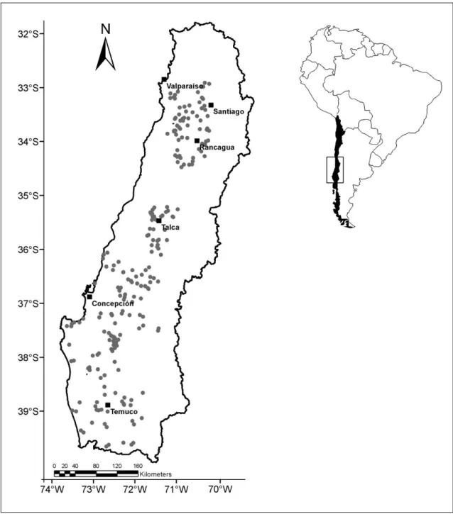
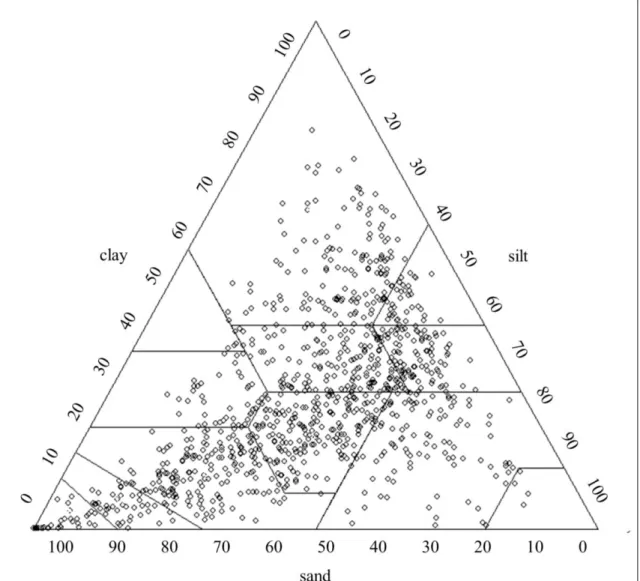
(20) 11. 3.. MATERIALS AND METHODS. 3.1.. Soil samples. The soil samples used in this study came from a series of soil surveys performed by the Natural Resources Information Center CIREN (1996a, 1996b, 1997a, 1997b, 1999, 2002) from Chile’s Ministry of Agriculture between the years 1971 and 1983. The location of the sampled sites extended from latitudes 32°S to 40°S and longitudes 70° to 73°W and covered the central region of Chile (Fig. 2), which has a wide range of climate conditions (Bonilla and Vidal, 2011). Most of the study area is in the Central Valley, a geological plain between the Western Andes Mountains and the coastal range that extends for approximately 1,000 km from the Valparaíso Region south to the Araucanía Region. This plain is approximately 70 km wide and is composed of a vast thick deposit of heavily mineralized alluvial soils formed by the principal rivers of the region (Bonilla and Johnson, 2012). Most farmland (72%) and national forest areas (54%) of the country are concentrated in this area (INE, 2007). A total of 1,007 soil samples with ρb data (from 243 soil series) were identified in the study area. The samples corresponded to seven soil orders: Alfisols (26 series, 106 horizons), Andisols (41 series, 181 horizons), Inceptisols (74 series, 313 horizons), Mollisols (83 series, 334 horizons), Entisols (10 series, 37 horizons), Ultisols (7 series, 29 horizons), and Vertisols (2 series, 7 horizons). The 1,007 samples covered the 12 USDA soil textures (Fig. 3). A summary of the soil properties is listed in Table 1..

(21) 12. Figure 2: Location of the soil data (soil pits) from soil surveys..

(22) 13. Table 1. Summary of properties of the soil samples used in the study.. Variable Sand fraction Silt fraction Clay fraction Bulk density (Mg m-3) Depth (m) θ33 (% grav.) θ1500 (% grav.) Organic carbon (%) Basic cations (cmol kg-1) pH. N. Mean. Median. Minimum (xmin). Maximum (xmax). Standard deviation. Coef. of variation (%). 1,007 1,007 1,007 1,007 1,007 754 754 1,007 880 997. 0.39 0.36 0.25 1.33 0.48 30.48 18.70 1.74 11.70 6.52. 0.34 0.36 0.24 1.37 0.41 27.00 16.00 1.02 9.67 6.40. 0.03 0.00 0.00 0.56 0.03 1.80 1.10 0.00 0.27 4.60. 1.00 0.85 0.78 2.10 2.25 107.27 63.60 13.03 43.10 9.20. 0.23 0.16 0.16 0.36 0.34 16.78 11.66 2.03 8.79 0.81. 59 43 62 27 71 55 62 117 75 12.

(23) 14. Figure 3: Soil texture distribution among the 1,007 soil samples used in the study..

(24) 15. The soil analysis at the time of the field surveys was conducted according to the standard soil methods used in Chile (INIA, 2006). The ρb was determined by the clod method (Blake and Hartge, 1986), and the particle size distribution was determined by the Bouyoucos method (Bouyoucos, 1962) according to the USDA textural classification (sand 2-0.05 mm; silt 0.05-0.002 mm; clay <0.002 mm). The OC content was measured by the dichromate method (Walkley and Black, 1934), and the OM content was obtained by multiplying the OC value by the Van Bemmelen factor of 1.724 (Davis, 1974). The pH was measured by suspension and potentiometric determination (proportion 1:1 soil/water), the water retention parameters (θ1500 and θ33) by the pressure plate method (Klute, 1986), and the calcium, magnesium, and potassium contents were measured using extraction with an ammonium acetate solution of 1 mol L-1 at pH 7.0 and spectrophotometric determination with atomic absorption and emission (using lanthanum suppression) (INIA, 2006).. 3.2.. Artificial neural networks. The hierarchical approach for predicting ρb using ANN was developed by building six different networks (named A to F) based on the type and number of input parameters collected from the literature. The first network (A) used sand, silt, and clay content as inputs, whereas the second network (B) used only OM content as input. The network C was a combination of networks A and B: it used sand, silt, and clay content in addition to the OM content. Networks D, E, and F used the same parameters as network C but included pH, basic cations, and soil depth and θ1500, respectively, as inputs. The ANN were built with a two-layer feed forward network (hidden layer and output layer) using the Levenberg-Marquardt back-propagation algorithm as the training function (Hagan and Menhaj, 1994). The transfer function used was a hyperbolic tangent sigmoid, and the performance function was the mean square error (MSE). The soil samples were randomly divided into three sets: (i) training (70%), (ii) validation (15%), and (iii) testing (15%). The training and validation sets were used to develop the.

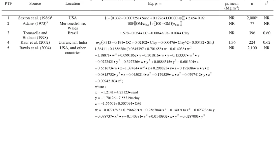
(25) 16. network, and the testing set was used to evaluate the equation independently of the development of the network. Every time an ANN was executed a different solution for the same problem was generated because of the randomization of these three sets (Tamari et al., 1996). For this reason, a total of 100 iterations were performed and the targets of the ANN were the measured ρb values. All simulations were performed with the neural network toolbox of MATLABTM (The MathWorks Inc., USA). The number of nodes in the hidden layer is commonly estimated based on the number of inputs (HechtNielsen, 1987; Sheela and Deepa, 2013); however, different numbers of nodes were tested (from 1 to 15) in this study in search of the optimal performance of the ANN, which generated 1,500 iterations per network. The criteria for choosing the best iteration per network were: (i) to obtain predicted values in the ρb range (from 0 to approximately 2.5 Mg m-3), (ii) the MSE for training and validation must be the lowest, and (iii) the maximum and minimum values of the input variables must be part of the training set (Tamari et al., 1996). To reduce the “black box” effect usually associated with the ANN structure (Olden and Jackson, 2002) and to isolate the contribution of each input variable within the network, the Relative Importance (RI) of each input parameter in the ANN was computed using the algorithm developed by Garson et al. (1991) and described in detail by Olden and Jackson (2002).. 3.3.. Equations tested for predicting soil bulk density. Ten already existing PTFs were selected for comparing their performance with those developed with the ANN technique. These PTFs were chosen considering: (i) their being built with soil data from different territories or a wide range of soil types, (ii) their use of different numbers of input variables, and (iii) their generation based on relatively large sample sets. These 10 PTFs were grouped in the same categories as the equations developed with the ANN (from A to F) based on the inputs..

(26) 17. The main characteristics of each are listed in Table 2. As suggested by De Vos et al. (2005), all the available horizons were used for testing the PTFs. The PTFs were tested in their original (without calibration) and calibrated forms. The calibration procedure consisted of computing the equation constants by minimizing the Root Mean Square Error (RMSE) (Eq. 1) between the estimated and measured ρb values. Specifically, the Rawls et al. (2004) equation was evaluated for A-horizons (because this equation was developed for this soil layer) and also for the entire set of samples. On the other hand, the Brahim et al. (2012) equation uses the sand content computed for soil particles between 0.20 to 2 mm; because the same range was not available in this soil dataset, the closest range (between 0.25 and 2 mm) was used instead..

(27) 18. Table 2. Pedotransfer functions evaluated in the study. Sample sizes (n), mean ρb and r2 values from the original publications. PTF Source Location Eq. ρb =. 1 2. Saxton et al. (1986)1 Adams (1973)3. 3. Tomasella and Hodnett (1998) Kaur et al. (2002) Rawls et al. (2004). 4 5. USA Merionethshire, Wales Brazil Utaranchal, India USA, and other countries. ρb mean (Mg m-3). n. r2. 1  0.332  0.0007251 Sand + 0.1276  LOGClay  2.65 0.92 100/ OM/ b,o  + 100  OM / b,m . NR NR. 2,0002 77. NR NR. 1.578  0.054  OC  0.006  Silt  0.004  Clay. NR. 396. 0.60. 1.36 NR. 224 2,100. 0.62 NR. exp0.313  0.191 OC + 0.02102  Clay  0.000476  Clay^2  0.00432  Silt. 1.36411+ 0.185628  (0.0845397 + 0.701658  w  0.614038  w. 2.  1.18871 w 3 + 0.0991862  y  0.301816  w  y  0.153337  w 2  y  0.0722421 y 2 + 0.392736  w  y 2 + 0.0886315  y 3  0.601301 z + 0.651673  w  z  1.37484  w 2  z + 0.298823  y  z  0.192686  w  y  z + 0.0815752  y 2  z  0.0450214  z 2  0.179529  w  z 2  0.0797412  y  z 2 + 0.00942183  z 3 ) where : x = 1.2141+ 4.23123  sand y = 1.70126 + 7.55319  clay z = 1.55601 + 0.507094  OM w = 0.0771892 + 0.256629  x + 0.256704  x 2  0.140911 x 3  0.0237361 y  0.098737  x 2  y  0.140381 y 2 + 0.0140902  x  y 2 + 0.0287001 y 3.

(28) 19. Table 2. Continued PTF Source. 6. Hollis et al. (2012). 7 8 9 10. Bernoux et al. (1998) Brahim et al. (2012) Benites et al. (2007) Heuscher et al. (2005). Location. Europe. Eq. ρb =.  0.750636  exp  0.230355  OC    0.69794 +   + 0.0008687  Sand   0.0005164  Clay 1.524  0.0038  Clay  0.05  OC  0.045  pH + 0.001 Sand 1.65  0.117  OC  0.0042  Clay  0.0036  CoreSand + 0.031 pH 1.56  0.0005  Clay  0.01 OC + 0.0075  BC. ρb mean (Mg m-3). n. r2. 1.27. 925. NR. Brazil 1.18 323 Tunez 1.61 348 Brazil 1.36 1,396 USA, and NR 47,015 1.685  0.198  OC^0.5  0.0133  1500 + 0.0079  Clay + neighboring 0.00014  Depth  0.0007  Silt countries 1 According to del Grosso’s modification used in Century Model 4.0 (https://www.nrel.colostate.edu/projects/century/). 2 Personal communication. 3 Adams (1973) used ρb,o=0.224 Mg m-3 and ρb,m=1.27 Mg m-3. NR: Not reported. Sand (%) (fraction in Saxton et al., 1986; and in Rawls et al., 2004). Silt (%), Clay (%) (fraction in Saxton et al. (1986); and in Rawls et al., 2004; and g kg-1 in Benites et al., 2007). OC: organic carbon content (%) (g kg-1 in Benites et al., 2007). OM: organic matter content (%). CoreSand (%): range [0.2-2] mm. BC: basic cations (cmol kg-1). ρb: soil bulk density (Mg m-3). θ1500: soil water content at wilting point (% grav.). Depth (cm).. 0.56 0.55 0.66 0.44.

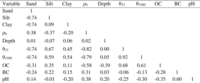
(29) 20. 3.4.. Statistical analysis. The correlation between the variables in the soil dataset was assessed by computing the coefficient of Pearson (r). Additionally, the r2, RMSE, and the Nash-Sutcliffe Model Efficiency (ME) were used to test the predictive capabilities of the equations developed with the ANN and the existing PTFs. The RMSE and the ME were computed as follows:. n.  ( yˆ. i. - yi ) 2. i =1. RMSE =. (1). n n.  ( yˆ ME = 1 -. i. - yi ) 2. i =1 n.  (y - y ). (2) 2. i. i =1. where yi and ŷi are the measured and predicted ρb values, respectively; y is the mean of measured values; and n is the number of observations. The r2 is a measure of the strength of the linear relationship between the measurements and predictions and indicates the fraction of the variation that is shared between them (De Vos et al., 2005). The RMSE is a measure of the overall error of the prediction, and the ME is a measure of the accuracy of the prediction and indicates how much the fit is related to the 1:1 line. Ideally, the r2 and ME should be close to 1 and the RMSE close to 0..

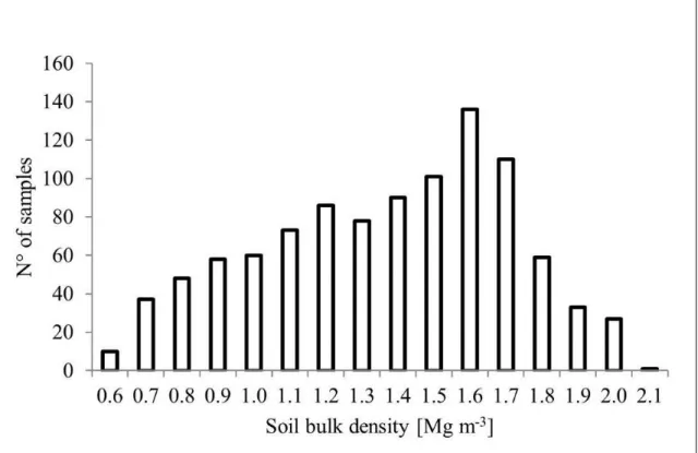
(30) 21. 4.. RESULTS AND DISCUSSION. The main results of this study were (i) a description of the soil properties in the sample dataset, (ii) a description of the ANN networks developed and the characterization of the RI of their input parameters, (iii) the development of a new and hierarchical set of equations for estimating ρb using the ANN, (iv) a comparison of the performance of the 10 PTFs collected from literature both without calibration and calibrated, and (v) a comparison between the equations developed with the ANN and the calibrated PTFs.. 4.1.. Soil properties in the soil data set. The mean ρb value in the soil dataset was 1.33 Mg m-3 (Table 1). As shown in Fig. 4, the histogram of ρb values did not show a normal distribution (p<0.005 by the AndersonDarling test) and most of the ρb were between 1.2 and 1.8 Mg m-3 (65% of the samples). The OC content in the samples ranged from 0.00 to 0.13, with a coefficient of variation (CV) of 117% (Table 1); as has been reported in previous studies (Bernoux et al., 1998; Brahim et al., 2012), this high CV value is because OC content is highly variable in soils..

(31) 22. Figure 4: Soil bulk density histogram for the soil samples (n=1,007).. Table 3 shows the matrix of correlation among the soil properties based on the data from Table 1. When analyzing the entire soil sample set (n=1,007), the ρb value decreased as the OC content increased (r=−0.58). Despite diverse studies that have reported OC content as the main input parameter explaining the variation in ρb, OC content in this dataset explained only 34% of the variation in ρb. This low OC predictor score was caused by the low values of OC content (Table 1), which was also shown by Bernoux et al. (1998). In fact, the functions that used OC content as a main (or sole) input were developed in soils with high OC contents. Those studies included Curtis and Post (1964), Adams (1973), Alexander (1980), and Huntington et al. (1989). The study of Leonaviciute (2000) found that ρb changes with soil depth, whereas other studies have reported that these two soil properties are independent (Heuscher et al., 2005; Martin et al., 2009). The low Pearson coefficient with soil depth (r=-0.01) endorses the results of Heuscher et al. (2005) and Martin et al. (2009). Additionally, the differences in the ρb mean for each soil horizon in the soil dataset were not statistically significant. A low correlation was found between ρb and clay, silt, and sand content (r=−0.20 r=−0.37.

(32) 23. r=0.38, respectively). In contrast, the correlation was higher with θ33 and θ1500 than with other soil properties (r=−0.82 and r=−0.79, respectively), the same result as was reported by Patil and Chaturvedi (2012) when they predicted ρb in waterlogged soils. This high negative correlation was caused by the fact that more water retention at specific suction requires more available pore space and thus more porosity and, consequently, a small ρb.. Table 3. Correlation matrix (with the Pearson coefficient) between soil properties of Table 1 for the entire soil sample set.. ρb. Depth. θ33. θ1500. Variable Sand Silt Clay. Sand 1 -0.74 -0.74. Silt. Clay. 1 0.09. 1. ρb. 0.38. -0.37. -0.20. 1. Depth. 0.01. -0.07. 0.06. 0.02. 1. θ33. -0.74. 0.67. 0.45. -0.82. 0.00. 1. θ1500. -0.74. 0.59. 0.54. -0.79. 0.05. 0.92. 1. OC BC pH. -0.31 -0.24 0.14. 0.35 0.22 -0.01. 0.11 0.15 -0.20. -0.58 0.31 0.38. -0.39 0.03 0.20. 0.68 -0.06 -0.25. 0.61 -0.13 -0.30. OC. 1 -0.28 -0.35. BC. pH. 1 0.60. 1. ρb: soil bulk density. θ33: soil water content at field capacity. θ1500: soil water content at wilting point. OC: organic carbon. BC: basic cations.. 4.2.. Artificial neural networks. The ANN developed for predicting ρb had three steps (pre-processing, neural network, and post-processing). After testing a wide range of numbers of nodes, no statistically significant improvement in the r2 values was found when using four or more nodes in each type of equation. Therefore, the equations were built with three nodes and the input for equations A to F. The pre-processing (input variables standardization) was accomplished by using the following equation:.

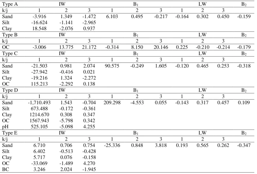
(33) 24. xp = ( xp max  xp min )/( x max  x min )  ( x  x min ) + xp min. (3). where xp is the standardized input variable, xpmin and xpmax are the minimum and maximum values for xp (equal to -1 and 1, respectively), x is the input value of the variable, and xmin and xmax are the minimum and maximum values for the input variable. The values for xmin and xmax are listed in Table 1 for each variable. The general form of the neural network is presented in Eq. 4. The normalized inputs xpk (k=1 to K) for the node j (j=1 to 3) are multiplied by the weights IWjk and summed with the bias term b1j. Then, the sigmoid function is applied and multiplied by the layer weights (LWj) and summed together with the constant b2 to generate the output a2 as follows:. 3. a2 =.  j=1. K.  IW. LW j  tansig(. jk.  xp k + b1j ) + b2. (4). k =1. where the values for LWj, IWjk, b1j, and b2 are listed in Table 4 to write and use the equations. Because the output a2 is standardized, it must be reverse-processed to obtain the predicted values. This is accomplished by using Eq. 5: yˆ = ( yˆ max  yˆ min )/(a 2 max  a 2 min )  (a 2  a 2 min ) + yˆ min. (5). where ŷ is the predicted ρb value, ŷmax and ŷmin are the maximum and minimum value of ŷ (2.1 and 0.56 Mg m-3 for this soil set, respectively), a2max and a2min are 1 and -1, respectively, and a2 is the network output of Eq. 4..

(34) 25. Table 4. Values of parameters LWj, IWjk, b1j and b2 for the Artificial Neural Network equations.. Type A k/j Sand Silt Clay Type B k/j OC Type C k/j Sand Silt Clay OC Type D k/j Sand Silt Clay OC pH Type E k/j Sand Silt Clay OC BC. 1 -3.916 -16.624 18.548 1 -3.006 1 -21.503 -27.942 -19.216 115.213 1 -1,710.493 673.488 1214.670 1567.943 525.105 1 6.710 6.402 5.717 -33.069 3.246. IW 2 1.349 -1.141 -2.076 IW 2 13.775 IW 2 0.981 -0.416 1.324 -2.292 IW 2 1.543 -0.172 0.308 -5.798 -5.098 IW 2 0.706 -0.513 0.076 -1.489 2.024. B1 2 0.495. 3 -1.472 -2.965 0.937. 1 6.103. 3 21.172. 1 -0.314. 3 2.074 0.021 -2.272 0.138. 1 90.575. B1 2 8.150 B1 2 -0.249. 1 209.298. B1 2 -4.553. 1 -25.336. B1 2 0.848. 3 -0.704 -0.361 0.347 0.342 4.255 3 0.754 -0.428 -0.158 4.270 -1.945. LW 2 0.302. 3 -0.217. 1 -0.164. 3 20.146. 1 0.225. 3 1.605. 1 -0.120. LW 2 -0.210 LW 2 0.465. 1 -0.143. LW 2 0.317. 1 0.193. LW 2 0.565. 3 0.055. 3 3.818. B2 3 0.450. -0.159. B2 3 -0.214 3 0.253. -0.179 B2 -0.318. B2 3 0.457. 0.109. B2 3 0.262. -0.347.

(35) 26. Table 4. Continued. Type F k/j Sand Silt Clay OC Depth θ1500. 1 -0.541 -0.362 0.668 -0.850 0.070 -1.828. IW 2 212.413 279.561 165.583 0.137 109.134 82.895. 3 0.799 0.265 -1.525 0.398 -0.854 2.256. 1 -0.998. B1 2 -866.738. 3 0.547. 1 1.391. LW 2 0.144. B2 3 0.862. -0.176.

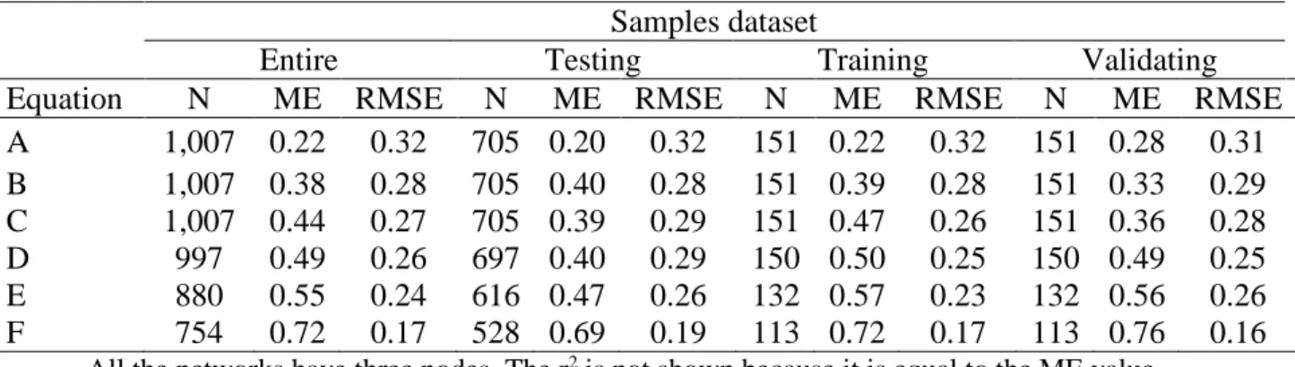
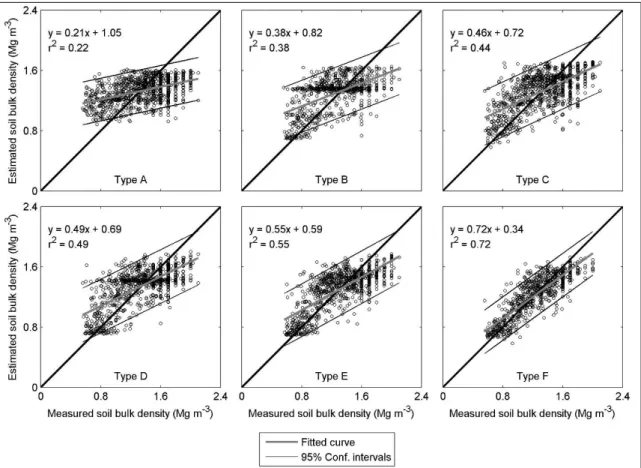
(36) 27. The RI of the variables showed that in equation A, the three inputs (sand, silt, and clay) had almost the same contribution (RI=34%, 34%, and 32%, respectively). For equation C and D, the most important input was the clay content (RI=35% and 32%, respectively). However, clay had the lowest correlation with ρb among the inputs of equation C and D (Table 3), which proved that the effect of clay was relevant but nonlinear in these equations. However, for equation E and F, OC content was the most significant input (RI=31% and 22%, respectively) and is consistently with the fact that OC content showed the highest correlation with ρb within the inputs of equation E. However, in the case of equation F, OC content has not the highest correlation with ρb among their inputs (Table 3), which proved that the effect of OC content was relevant but non-linear in this equation. The results of the RI analysis on input variables indicate that the process of estimating ρb cannot be explained for a single variable and cannot be simplified to a correlation analysis.. In terms of network performance, Table 5 shows the ME and RMSE obtained with the ANN for the entire sample dataset and the training, validating and testing sample sets. The relationships between the measured and predicted ρb are shown in Fig. 5. These equations were developed with measured ρb values in the range of 0.56 to 2.1 Mg m-3 (Table 1) and the estimates can be different when using for soils out of this range.. Table 5. Evaluation for equations A through F developed with the Artificial Neural Network techniques.. Equation A B C D E F. Entire N ME 1,007 0.22 1,007 0.38 1,007 0.44 997 0.49 880 0.55 754 0.72. RMSE 0.32 0.28 0.27 0.26 0.24 0.17. N 705 705 705 697 616 528. Samples dataset Testing Training ME RMSE N ME RMSE 0.20 0.32 151 0.22 0.32 0.40 0.28 151 0.39 0.28 0.39 0.29 151 0.47 0.26 0.40 0.29 150 0.50 0.25 0.47 0.26 132 0.57 0.23 0.69 0.19 113 0.72 0.17. Validating N ME RMSE 151 0.28 0.31 151 0.33 0.29 151 0.36 0.28 150 0.49 0.25 132 0.56 0.26 113 0.76 0.16. All the networks have three nodes. The r2 is not shown because it is equal to the ME value..

(37) 28. Figure 5: Comparison between measured soil bulk density (Mg m-3) and predicted values using the equations developed with the ANN technique for the entire soil sample set. The lines around the fitted curve are the 95% confidence intervals.. The performance of the equations improved (accuracy and overall error) as the number of inputs increased (from A to F). The lowest performance was found with equation A, which used only sand, silt, and clay content (ME=0.22, RMSE=0.32 Mg m-3). This is explained because sand, silt, and clay were not highly correlated with ρb (Table 3). In contrast, equation B, with only OC content, performed better than equation A (ME=0.38, RMSE=0.28 Mg m-3). This result indicates that an equation based on OC (or OM) provides better ρb estimates than a soil particle size distribution-based equation, even when applied to soils with low OC (or OM) content such as those used in this study. Equation C, which used OC, sand, silt, and clay content, had better performance for accuracy but was just slightly better for overall error compared with equation B (ME=0.44, RMSE=0.27 Mg m-3). Moreover, the performance improvement between.

(38) 29. equations B and C was smaller compared with the increment between equations A and B. However, a significant improvement was found when pH (equation D, ME=0.49, RMSE=0.26 Mg m-3) and basic cations (equation E, ME=0.55, RMSE=0.24 Mg m-3) were included. The best estimates were found when using equation F, with the highest ME (0.72) and the lower RMSE (0.17 Mg m-3). Differently from the other equations, equation F uses θ1500 and a high correlation was found between ρb and θ1500 (Table 3). Based on 332 soil samples, Al-Qinna and Jaber (2013) used ANN to develop an equation for predicting ρb based on OC, sand, silt, and clay content (the same as equation C). Using six nodes, their results showed an r2 and RMSE of 0.63 and 0.11 Mg m-3, and 0.27 and 0.14 Mg m-3 in calibration and validation, respectively. Their results had a higher r2 and a lower RMSE compared with this study. Their soils were more compacted (mean ρb = 1.68 Mg m-3) and had less variability (CV of 10%). On the other hand, Xiangsheng et al. (2016) used 495 soil samples as well as ANN to develop three equations for predicting ρb. Depending on the inputs, they obtained r2=0.69 and RMSE=0.15 when using OC content, r2=0.71 and RMSE=0.14 when clay and silt were added, and r2=0.71 and RMSE=0.14 when the soil depth was added to the previous variables. Their results showed better r2 and RMSE values compared with the results presented in this study although the soils used in their study were almost negligible in clay (mean of 0.01). However, their results showed the same pattern as this study; the performance of the equations improved with the number of inputs, even though the increments were very small. An analysis based on textural classes was also performed with the ANN. All the equations overestimated the ρb values when measured ρb was low (silt loam, silty clay, and silty clay loam) and underestimated the values when measured ρb was high (sand, loamy sand, and sandy clay loam)..

(39) 30. 4.3.. Evaluation of the previous PTFs. The performance of the 10 previous PTFs without calibration and calibrated is shown in Table 6 for the entire soil dataset. The comparison between the measured and predicted ρb values for the calibrated PTFs is shown in Fig. 6. Without calibration, all the equations overestimated ρb when the measured value was low. Only the equations developed by Bernoux et al. (1998), Tomasella and Hodnett (1998), and Heuscher et al. (2005) could predict ρb values as low as 0.60 Mg m-3. On the other hand, the equations consistently underestimated ρb when the measured value was high, and only the Saxton et al. (1986) and Heuscher et al. (2005) equations could predict values as high as 2 Mg m-3..

(40) 31. Table 6. Performance of the tested pedotransfer functions using the entire soils dataset.. PTF. 1 2 3 4 5a 5b 6 7 8 9 10. Eq.. A B C C C C C D D E F. Reference. Saxton et al. (1986) Adams (1973) Tomasella and Hodnett (1998) Kaur et al. (2002) Rawls et al. (2004)-A horizons Rawls et al. (2004)-All horizons Hollis et al. (2012) Bernoux et al. (1998) Brahim et al. (2012) Benites et al. (2007) Heuscher et al. (2005). n. 1,007 1,007 1,007 1,007 167 632 1,007 997 901 880 754. Without calibration r ME RMSE. Calibrated ME RMSE. Mg m-3. Mg m-3. 2. 0.05 0.36 0.36 0.38 0.39 0.26 0.38 0.25 0.33 0.22 0.43. The r2 in the calibrated section is not shown because is equal to the ME value.. -0.03 -0.02 0.13 -0.51 0.28 0.23 0.33 -0.25 0.16 -0.61 0.24. 0.36 0.36 0.33 0.44 0.24 0.30 0.29 0.40 0.34 0.46 0.29. 0.17 0.36 0.39 0.41 0.48 0.32 0.39 0.42 0.44 0.41 0.67. 0.33 0.29 0.28 0.28 0.21 0.28 0.28 0.27 0.27 0.28 0.19.

(41) 32. Figure 6: Comparison between measured soil bulk density (Mg m-3) and predicted values with the existing pedotransfer functions calibrated for the entire soil sample set. The lines around the fitted curve are the 95% confidence intervals.. The estimates showed an ME between -0.61 and 0.33. The equations developed by Adams (1973), Saxton et al. (1986), Bernoux et al. (1998), Kaur et al. (2002), and Benites et al. (2007) showed negative ME values, which means that it is better to use the average ρb value of the soil dataset of this study instead these equations. However, the calibration reduced the difference between the predicted and measured ρb values, with an ME between 0.17 and 0.67. The RMSE for these equations without calibration was between 0.29 Mg m-3 and 0.46 Mg m-3. With a ρb mean of 1.33 Mg m-3, the RMSE was between 19% and 35% of the mean ρb. The calibration reduced the overall prediction error to between 0.19 Mg m-3 and 0.33 Mg m-3, or between 14% and 25% of the mean ρb ..

(42) 33. When the equations were calibrated with this new soil dataset, the performance followed the same trend as the equations developed with ANN in section 3.2: the estimates improved with the number of inputs in the equations. The estimates that differed more from the measured ρb values were obtained with equation A (Saxton et al., 1986), which used only sand and clay. Equations C (Tomassella and Hodnett, 1998; Kaur et al., 2002; Rawls et al., 2004 and Hollis et al., 2012), which used OC (or OM) and sand, silt and/or clay, had similar accuracy and overall error (Table 6) and provided better estimates than equation A. In terms of ME, equation B (Adams, 1973) was similar to equations C but with a larger overall error as a result of using only OM content as input (RMSE=0.34 Mg m-3). Compared with equation C, and differently from the relationships developed with the ANN, no significant improvement in the quality of the estimates was observed when pH was added (equation D: Bernoux et al., 1998 and Brahim et al., 2012) or basic cations were added (equation E: Benites et al., 2007). However, the best estimates were obtained with equation F (Heuscher et al., 2005). The ME and RMSE demonstrated that this PTF was the most reliable for this soil dataset when predicting ρb. The other PTFs showed some limitations when tested on Chilean soils as reported by Casanova et al. (2016) after testing 10 PTFs in two soils of Central Chile. In the case of equations C, the PTF developed for the A-horizons (Rawls et al., 2004) worked better for those horizons than when used to predict ρb in the entire soil profile. However, when compared with the other equations C, the estimates were similar in RMSE and better in ME. This improvement in accuracy was highly related to complex combinations of variables in the original equation (Table 2). Moreover, to remove any possible bias related to the number of samples used in the comparison, an additional test was performed for all the PTFs with the same number of soil samples (n=611). The results were not significantly different from those presented in Table 6 when using different number of soil samples. Furthermore, the calibrated form of the PTFs evaluated are shown in Table 7 for practical use..

(43) 34. Table 7. Mathematical form of the calibrated pedotransfer functions developed in this study. PTF. Source. 1 2 3 4 5. Saxton et al. (1986) Adams (1973) Tomasella and Hodnett (1998) Kaur et al. (2002) Rawls et al. (2004). Eq. ρb =. 1  0.708  0.004  Sand + 0.076  LOGClay  2.65 0.959 100/ OM/ 0.181 + 100  OM/1.586 1.710  0.089  OC  0.004  Silt  0.003 Clay exp0.332  0.087  OC + 0.006  Clay  0.0001 Clay^2  0.003 Silt. 1.303 + 0.223  (0.088 + 3.085  w  1.075  w 2  4.223  w 3 + 0.491 y  1.473  w  y  0.290  w 2  y 0.333  y 2 + 0.606  w  y 2 + 0.084  y 3  0.335  z + 0.844  w  z  1.308  w 2  z + 0.113  y  z  0.090  w  y  z + 0.139  y 2  z  0.219  z 2  0.254  w  z 2  0.058  y  z 2 + 0.040  z 3 ) where : x = 1.2141+ 4.23123  sand y = 1.70126 + 7.55319  clay z = 1.55601 + 0.507094  OM w = 0.0771892 + 0.256629  x + 0.256704  x 2  0.140911 x 3  0.0237361 y. 6. Hollis et al. (2012). 7 8 9 10. Bernoux et al. (1998) Brahim et al. (2012) Benites et al. (2007) Heuscher et al. (2005).  0.098737  x 2  y  0.140381 y 2 + 0.0140902  x  y 2 + 0.0287001 y 3 1.142  exp  0.127  OC    0.238 +   + 0.003  Sand   0.0007  Clay 0.574  0.003 Clay  0.075  OC  0.097  pH + 0.005  Sand 0.639  0.075  OC  0.0006  Clay  0.004  CoreSand + 0.119  pH 1.477  0.004  Clay  0.09  OC + 0.008  BC 1.820  0.160  OC^0.5  0.015  1500 - 0.0006  Clay 0.002  Depth  0.001 Silt.

(44) 35. In addition, as shown in section 3.2, an analysis based on textural classes was also performed for the calibrated PTFs. As the equations developed with ANN, the same condition was found. However, equations C and D overestimated the ρb values in sandy soils, which indicates that these types of PTFs are less accurate in soils either with extremely high sand or low clay contents (0.94 and 0.01 on average, respectively).. 4.4.. Comparison between the ANN and the calibrated PTFs. The performance of the ANN was compared with those of the calibrated PTFs evaluated in section 3.3. This test provided a fair comparison because the constants in both groups of equations were computed with the same soil sample set. The results showed a better ME and RMSE in all the ANN compared with the already existing PTFs. The improvement in ME was between 0.02 and 0.14. However, the increment in the ME in equation B was not statistically significant after the Fisher test (p=0.24) because the ANN technique cannot significantly enhance the quality of estimates with one input (Hecht-Nielsen, 1990). Equations A, C, D, E, and F provided statistically significant improvements in the ME (p=0.04, p=0.04, p=0.04, p=0.00 and p=0.03, respectively) compared with the previous PTFs, which demonstrates the convenience of using the ANN technique compared with classical multivariable regression analysis. The highest increment in ME was with equation E, which proved the suitability of the use of basic cations as input compared with the use of pH in equation D. However, the improvement in the RMSE was not relevant (between 0.01 Mg m-3 and 0.04 Mg m-3) and the error was on the order of the error of the core and clod analytical methods (Blake and Hartge, 1986)..

(45) 36. 5.. CONCLUSIONS. The use of artificial neural network techniques proved to be a suitable method for building six equations for predicting ρb across a wide range of soil types and inputs. The ANN developed in this study were two-layer feed forward networks with 3 nodes, and their capability for predicting ρb was related to the number of parameters used in the network. The networks were established with the inputs of sand, silt and clay content (r2=0.22); organic carbon content (r2=0.38); sand, silt, clay and organic carbon content (r2=0.44); sand, silt, clay, organic carbon content and pH (r2=0.49); sand, silt, clay, organic carbon content and basic cations (r2=0.55); and sand, silt, clay, organic carbon content, depth and soil water content at wilting point (r2=0.72). Depending on the field and soil survey data, these ANN are meant to be selected and used hierarchically to predict ρb values. The inputs required for the networks are usually available in soil surveys, and the networks can be easily coupled with other soil and hydrology models to provide an alternative for estimating ρb when its measured value is not available. Compared with other existing PTFs developed for predicting ρb, the equations developed with ANN enhanced the quality of estimates when they were evaluated with the same type and number of input parameters. This condition demonstrates that this technique is a promising option for relationships for predicting variable soil properties such as bulk density. Although the classical regression relationships are still useful for predicting the soil bulk density because of their simplicity and intuitive formulation, the use of this new set of equations is highly recommended to produce a more robust estimate and reduce the overall error. The set of ρb values used in this study came from many soil horizons and pits and covered a wide range of soil types, including cultivated and forest soils, in addition to a variety of climate conditions. Finally, if the data are available, the network based on sand, silt, clay and organic carbon content, soil depth, and soil water at the wilting point should be used with the set of the equations presented in this study to obtain the best estimates..

(46) 37. REFERENCES Adams, W.A. 1973. The effect of organic matter on the bulk and true densities of some uncultivated podzolic soils. Journal of Soil Science 24:10-17. Alexander, E.B. 1980. Bulk densities of California soils in relation to other soil properties. Soil Science Society of America Journal 44:689-692. Al-Qinna, M.I., and S.M. Jaber. 2013. Predicting soil bulk density using advanced pedotransfer functions in an arid environment. Transactions of the American Society of Agricultural and Biological Engineers. 56(3): 963-976. Baker, L., and D. Ellison. 2008. Optimisation of pedotransfer functions using an artificial neural network ensemble method. Geoderma 144(1-2): 212–224. Blake, G.R., and K.H. Hartge. 1986. Bulk density. In: A. Klute, editor, Methods of soil analysis: Part 1. Physical and mineralogical methods. ASA and SSSA, Madison, WI. p. 371-373. Benites, V.M., P.L.O.A. Machado, E.C.C. Fidalgo, M.R. Coelho, and B.E. Madari. 2007. Pedotransfer functions for estimating soil bulk density from existing soil survey reports in Brazil. Geoderma 139:90–97. Bernoux, M., D. Arrouays, C. Cerri, B. Volkoff, and C. Jolivet. 1998. Bulk Densities of Brazilian Amazon Soils Related to Other Soil Properties. Soil Sci. Soc. Am. J. 62: 743749. Bonilla, C. and J. Cancino. 2001. Soil water content estimation using pedotransfer functions. Chilean Journal of Agricultural Research 61(3):326-338. (In Spanish) Bonilla, C.A., and K.L. Vidal. 2011. Rainfall erosivity in central Chile. Journal of Hydrology 401:126-133..

(47) 38. Bonilla, C. A., and O. I. Johnson. 2012. Soil erodibility mapping and its correlation with soil properties in Central Chile. Geoderma. 189-190:116-123. Boucneau, G., M. Van Meirvenne, and G. Hofman. 1998. Comparing pedotransfer functions to estimate soil bulk density in northern Belgium. Pedologie Themata. 5:6770. Bouyoucos, G.J. 1962. Hydrometer method improved for making particle size analysis of soils. Agronomy Journal. 54:464-465. Brahim, N., M. Bernoux, and T. Gallali. 2012. Pedotransfer functions to estimate soil bulk density for Northern Africa: Tunisia case. J. Arid Environ. 81:77–83. Brown, J. D. and Heuvelink, G. B. M. 2006. Assessing Uncertainty Propagation through Physically Based Models of Soil Water Flow and Solute Transport. Encyclopedia of Hydrological Sciences. 6:79. Calhoun, F.G., N.E. Smeck, B.L. Slater, J.M. Bigham, and G.F. Hall. 2001. Predicting bulk density of Ohio soils from morphology, genetic principles, and laboratory characterization data. Soil Sci. Soc. Am. J. 65:811-819. Casanova, M., E. Tapia, O. Seguel, and O. Salazar. 2016. Direct measurement and prediction of bulk density on alluvial soils of central Chile. Chilean Journal of Agricultural Research. 76(1):105-113. CIREN, 1996a. Estudio Agrológico. Descripción de suelos. Materiales y símbolos. Región Metropolitana. Centro de Información de Recursos Naturales. (In Spanish). CIREN, 1996b. Estudio Agrológico. Descripción de suelos. Materiales y símbolos. Región de Libertador B. O'Higgins. Centro de Información de Recursos Naturales. (In Spanish). CIREN, 1997a. Estudio Agrológico. Descripción de suelos. Materiales y símbolos. Región de Valparaíso. Centro de Información de Recursos Naturales. (In Spanish)..

(48) 39. CIREN, 1997b. Estudio Agrológico. Descripción de suelos. Materiales y símbolos. Región del Maule. Centro de Información de Recursos Naturales. (In Spanish). CIREN, 1999. Estudio Agrológico. Descripción de suelos. Materiales y símbolos. Región del Bío-Bío. Centro de Información de Recursos Naturales. (In Spanish). CIREN, 2002. Estudio Agrológico. Descripción de suelos. Materiales y símbolos. Región de la Araucanía. Centro de Información de Recursos Naturales. (In Spanish). Curtis, R.O., and B.W. Post. 1964. Estimating bulk density from organic matter in some Vermont forest soils. Soil Science Society of America Journal. 28:285-286. Dam, R.F., B.B. Mehdi, M.S.E. Burgess, C.A. Madramootoo, G.R. Mehuys, I.R. Callum. 2005. Soil bulk density and crop yield under eleven consecutive years of corn with different tillage and residue practices in a sandy loam soil in central Canada. Soil and Tillage Research. 84:41-53. Davis, B.E. 1974. Loss-on-ignition as an estimate of soil organic matter. Soil Science Society of America. Proceedings. 38:150-151. De Vos, B., M. Van Meirvenne, P. Quataert, J. Deckers, and B. Muys. 2005. Predictive Quality of Pedotransfer Functions for Estimating Bulk Density of Forest Soils. Soil Sci. Soc. Am. J. 69:500-510. Garson, G.D. 1991. Interpreting Neural-network Connection Weights. Artificial Intelligence Expert 6(4): 46-51. Hagan, M.T., and M.B. Menhaj. 1994. Training Feedforward Networks with the Marquardt Algorithm. IEEE Trans. Neural Networks 5(6): 989–993. Han, G-Z., G-L. Zhang, Z-T. Gong, and G-F. Wang. 2012. Pedotransfer Functions for Estimating Soil Bulk Density in China. Soil Sci. 177:158–164. Hecht-Nielsen, R. (1987). Kolmogorov’s Mapping Neural Network Existence Theorem..

(49) 40. In Proceedings of the IEEE First International Conference on Neural Networks, San Diego, CA, USA (11–13). Hecht-Nielsen, R. (1990). Neurocomputing. Addison-Wesley, Reading, MA. Heuscher, S. A, C.C. Brandt, and P.M. Jardine. 2005. Using Soil Physical and Chemical Properties to Estimate Bulk Density. Soil Sci. Soc. Am. J. 69:1–7. Hollis, J.M., J. Hannam, and P.H. Bellamy. 2012. Empirically-derived pedotransfer functions for predicting bulk density in European soils. Eur. J. Soil Sci. 63:96–109. Huntington, T.G., C.E. Johnson, A.H. Johnson, T.G. Siccama, and D.F. Ryan. 1989. Carbon, organic matter, and bulk density relationships in a forested spodosol. Soil Science. 148:380-386. INE, 2007. VII Censo Nacional Agropecuario y Forestal. Instituto Nacional de Estadística, Santiago, Chile. (In Spanish). INIA, 2006. Métodos de análisis recomendados para los suelos de Chile. Serie Actas INIA N°34, Santiago, Chile. (In Spanish). Jalabert, S.S.M., M.P. Martin, J.-P. Renaud, L. Boulonne, C. Jolivet, L. Montanarella, and D. Arrouays. 2010. Estimating forest soil bulk density using boosted regression modelling. Soil Use Manag. 26:516–528. Kaur, R., S. Kumar, and H.P. Gurung. 2002. A pedo-transfer function (PTF) for estimating soil bulk density from basic soil data and its comparison with existing PTFs. Aust. J. Soil Res. 40:847–857. Klute, A. 1986. Bulk density. In: A. Klute, editor, Methods of soil analysis: Part 1. Physical and mineralogical methods. ASA and SSSA, Madison, WI. p. 635-656. Koekkoek, E.J.W., and H. Booltink. 1999. Neural network models to predict soil water retention. Eur. J. Soil Sci. 50: 489–495..

(50) 41. Lagos-Avid M.P., and C.A. Bonilla. 2017. Predicting the particle size distribution of eroded sediment using artificial neural networks. Science of the Total Environment 581– 582:833–839. Leonaviciute, N. 2000. Predicting soil bulk and particles densities by pedotransfer functions from existing soil data in Lithuania. Geografijos Metrastis. 33:317-330. Martin, M.P., D. Lo Seen, L. Boulonne, C. Jolivet, K.M. Nair, G. Bourgeon, and D. Arrouays. 2009. Optimizing Pedotransfer Functions for Estimating Soil Bulk Density Using Boosted Regression Trees. Soil Sci. Soc. Am. J. 73:485-493. Merdun, H., Ö. Çınar, R. Meral, and M. Apan. 2006. Comparison of artificial neural network and regression pedotransfer functions for prediction of soil water retention and saturated hydraulic conductivity. Soil Tillage Res. 90(1-2):108–116. Nanko, K., S. Ugawa, S. Hashimoto, A. Imaya, M. Kobayashi, H. Sakai, S. Ishizuka, S. Miura, N. Tanaka, M. Takahashi, and S. Kaneko. 2014. A pedotransfer function for estimating bulk density of forest soil in Japan affected by volcanic ash. Geoderma. 213:36–45. Olden, J.D., and D.A. Jackson. 2002. Illuminating the “black box”: A randomization approach for understanding variable contributions in artificial neural networks. Ecological Modelling. 154(1-2): 135–150. Pachepsky, Y. A., Rawls, W.J. 1999. Accuracy and reliability of pedotransfer functions as affected by grouping soils. Soil Sci. Soc. Am. J. 63:1748-1757. Patil, N.G., and A. Chaturvedi. 2012. Estimation of bulk density of waterlogged soils from basic properties. Arch. Agron. Soil Sci. 58:499–509. Prévost, M. 2004. Predicting Soil Properties from Organic Matter Content following Mechanical Site Preparation of Forest Soils. Soil Sci. Soc. Am. J. 68:943-949..

(51) 42. Rawls, W.J., 1983. Estimating soil bulk density from particle size analysis and organic matter content. Soil Science. 135:123-125. Rawls, W.J., A. Nemes, and Y. Pachepsky. 2004. Effect of soil organic carbon on soil hydraulic properties. Dev. Soil Sci. 30(C):95–114. Saxton, K.E., W.J. Rawls, J.S. Romberger, and R.I. Papendick. 1986. Estimating generalized soil-water characteristics from texture. Soil Sci. Soc. Am. J. 50:1031-1036. Schaap, M.G., F.J. Leij, and M.T. Van Genuchten. 2001. ROSETTA: a computer program for estimating soil hydraulic parameters with hierarchical pedotransfer functions. Journal of Hydrology. 251:163 – 176. Sheela, K. G. and Deepa, S. N. (2013). Review on methods to fix number of hidden neurons in neural networks. Mathematical Problems in Engineering. 2013, 1-11. Suuster, E., C. Ritz, H. Roostalu, E. Reintam, R. Kõlli, and A. Astover. 2011. Soil bulk density pedotransfer functions of the humus horizon in arable soils. Geoderma 163:74– 82. Tamari, S., J.H.M. Wösten, and J.C. Ruiz-Suárez. 1996. Testing an artificial neural network for predicting soil hydraulic conductivity. Soil Science Society of America Journal. 60(6): 1732–1741. Tomasella, J., and M.G. Hodnett. 1998. Estimating soil water retention characteristics from limited data in Brazilian Amazonia. Soil Sci. 163:190–202. Tremblay, S., R. Ouimet, and D. Houle. 2002. Prediction of organic carbon content in upland forest soils of Quebec, Canada. Can. J. For. Res. 32(5): 903–914. Vasiliniuc, I., and C.V. Patriche. 2015. Validating soil bulk density pedotransfer functions using a Romanian dataset. Carpathian Journal of Earth and Environmental Sciences. 10:225–236..

(52) 43. Walkley, A.J., Black, I.A. 1934. Estimation of soil organic matter carbon by the chromic acid titration method. Soil Science. 37:38-39. Wösten, J.H.M., Y.A. Pachepsky, and W.J. Rawls. 2001. Pedotransfer functions: Bridging the gap between available basic soil data and missing soil hydraulic characteristics. J. Hydrol. 251:123 – 150. Xiangsheng, YI, LI Guosheng, and YIN Yanyu. 2016. Pedotransfer functions for estimating soil bulk density: a case study in the Three-River headwater Region of Qinghai Province, China. Pedosphere 26(3):362-373..

(53)