Development of vortex state in circular magnetic nanodots: Theory and experiment
8
0
0
Texto completo
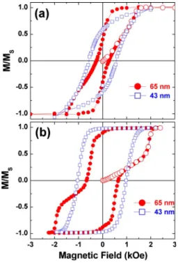
(2) PHYSICAL REVIEW B 81, 184417 共2010兲. MEJÍA-LÓPEZ et al.. FIG. 2. 共Color online兲 Ratio of the loop width at coercivity to the width at half saturation as a function of the dot diameter for 600 Monte Carlo steps 共after Ref. 14兲.. FIG. 1. 共Color online兲 Hysteresis loops for 43- 共squares兲 and 65共circles兲 nm-diameter, 20-nm-thick Fe dots at 10 K, and virgin curve 共empty circles兲 for the 65 nm dots: 共a兲 experimental data 共after Ref. 14兲; 共b兲 Monte Carlo simulations for the same conditions.. the theoretical calculations, respectively. Then, we discuss the magnetization-reversal mechanisms and present a detailed analysis of the microscopic structure of the vortex core. Finally, we compare the theoretical results with the experimental ones. In Sec. IV, we summarize our findings.. II. EXPERIMENT. Arrays of sub-100 nm Fe nanodots are prepared using electron-beam evaporation combined with lift-off of anodized alumina masks on silicon substrates.19 Powder x-ray diffraction shows that the hexagonally ordered Fe dots are polycrystalline. By controlling the anodization process 共i.e., electrochemical parameters兲 and using double anodization20 dot diameters and periodicities in the range 25–150 nm with narrow distributions 共10–15 standard deviation兲 are produced. The dot periodicity is typically nearly twice the dot diameter. The magnetic properties are determined from dc SQUID magnetometry and first-order reversal curves 共FORC兲 between 10 to 300 K and small angle-polarized neutron scattering in the range of the out-of-plane wave vector transfer, Qz, between 0.005 and 0.015 Å−1. Figure 1 shows 共a兲 experimental and 共b兲 simulated hysteresis loops for magnetic dots with 20 nm height and diameter D 共for clarity, only two diameters, 43 and 65 nm, are shown兲. For these sizes, the domain-wall width is comparable to the dot size; therefore, Fe dots with sub-100 nm diameters are not expected to form multidomain states.21 In this case, the coercivity and the equilibrium magnetic state depend on the. dot diameter. For very small diameters, the hysteresis loops strongly resemble curves described by Stoner-Wohlfarth model for reversal of single-domain elements.22 This can be seen for the 43-nm-diameter dots. Dots with diameters larger than ⬃60 nm show reduced coercivity, with a narrowing of the hysteresis loop close to the zero-magnetization states, as shown in Fig. 1 for the 65-nm-diameter dots. To quantify the effects of dot size on the hysteresis loop shape, we introduce the parameter ␦ = ⌬0.0 / ⌬0.5, with ⌬0.0 and ⌬0.5 the widths of the hysteresis loop at M = 0 共zero magnetization兲 and M = 0.5M s 共half saturation兲, respectively, M s being the saturation magnetization. Figure 2 shows the dependence of ␦ on the dot diameter obtained from both the experimental loops 共hollow red squares兲 and Monte Carlo simulations 共full green circles兲, described below. For dot diameters around 65 nm, this ratio is greatly reduced. This is typical for reversal via a vortex state as also observed with FORC measurements,23 confirmed by simulations9 and discussed in detail in the theoretical section below. The virgin curve measured from the as-grown state 共never exposed to magnetic field兲 or after demagnetization by field cycling about minor hysteresis loops is almost linear in a large field range. For diameters larger than 60 nm it joins the major hysteresis loop 共see Fig. 1兲. This very unusual behavior is in a good agreement with the results of Monte Carlo simulations.9 Below, we will focus on an array of Fe dots of average diameter of 65⫾ 7 nm with spacing of 110⫾ 12 nm and thickness of 20 nm covering a ⬃1.8 cm2 共Fig. 3兲. Since for these dots 共at the deep minimum in Fig. 2兲 the ground state is expected to be a vortex, we performed grazing incidence small angle neutron scattering with polarization analysis 关polarized grazing incidence small-angle neutron scattering 共GIS-ANS兲兴 to measure the perpendicular magnetization, M z, of the vortex core and its diameter.14 For these measurements, the sample is magnetically conditioned using the following protocol. First, a small, 34 Oe, field is applied along the surface normal of the sample 共along +ẑ兲 to set the preferred direction for the vortex-core magnetization 共core polarity兲. Next, a second field of −4 kOe is applied in the sample plane 共along −ŷ兲 to saturate the dots. Then the inplane field is slowly increased to +300 Oe—a field that ex-. 184417-2.
(3) PHYSICAL REVIEW B 81, 184417 共2010兲. DEVELOPMENT OF VORTEX STATE IN CIRCULAR…. energy, Etot, of a single dot with N magnetic moments is given as Etot =. 1 兺 共Eij − Jijˆ i · ˆ j兲 + EH , 2 i⫽j. 共1兲. where Eij is the dipolar energy as Eij = 关 ជi · ជ j − 3共 ជ i · n̂ij兲共 ជ j · n̂ij兲兴/r3ij. FIG. 3. 共Color online兲 共a兲 Scanning electron microscope image of the sample fabricated for neutron-scattering experiment. 共b兲 Distribution of the dot diameters. Average diameter 65⫾ 8 nm.. ceeds the vortex nucleation field 共Fig. 1兲—before returning this field to zero, leaving only the 34 Oe out-of-plane field.24 These quantitative measurements yield the out-of-plane magnetization of the dot in the vortex state, i.e., the magnetization of the vortex core, 140⫾ 50 emu/ cm3. An equivalent Fe cylinder with the same magnetization would have a diameter of 19⫾ 4 nm. Very similar numbers are obtained by modeling the vortex core with a different, more realistic spatial distribution of spins 共for instance, a circular Gaussian function, paraboloid, etc.兲. III. THEORETICAL CALCULATIONS. The geometry implies that these dots can be modeled as noninteracting 共i.e., without dipolar, exchange, or other couplings兲 due to their large separation.9,19,25–27 Earlier calculations have shown that when the side-to-side distance in an array is larger than a single-dot diameter 共i.e., the center-tocenter distance larger than twice the diameter兲 the dots interact weakly.9 Since the dots are polycrystalline, we neglect the crystalline anisotropies. Thus, both in the Monte Carlo simulation and analytical calculations we use these assumptions as a starting point. A. Monte Carlo simulations. Since the methods used here are standard, here we only review the main concepts used for the simulations.9 The total. 共2兲. with rij the distance between the magnetic moments ជ i and ជ j and n̂ij the unit vector along the direction that connects the two magnetic moments. Jij is the exchange coupling, ˆi which is assumed nonzero only for nearest neighbors and ជ is the is a unit vector along the direction of ជ i. EH = −兺i ជ i·H Zeeman energy. Because of the large number of magnetic moments within each particle, a brute force calculation of the magnetic configuration of a 10–100 nm structure is unreachable with present standard computational facilities even using the above-mentioned phenomenological energy function. To avoid this problem we use a scaling technique developed by d’Albuquerque e Castro et al.15 in which the number of spins is reduced to a value suitable for numerical calculations. This procedure decreases the dipolar field exerted on a particle, and therefore the exchange coupling constant is scaled down to keep the correct balance between magnetostatic and exchange energies, responsible for domain formation and reversal mechanisms. With this procedure15,18 the magnetic properties of a nanoparticle of dimensions d is equivalent to the one of a smaller particle with dimensions d⬘ = dx being x ⬍ 1 and ⬇ 0.55– 0.57, if the exchange constant is also scaled as J⬘ = xJ. This scaling method, in combination with Monte Carlo simulations,16,18 provides the correct magnetic state of a single nanoparticle. This approach was tested using different values of the scaling parameter x and the results were shown to be independent of it.15,18 This method applied to granular Fe, using 兩 ជ i兩 = = 2.2B, a lattice parameter a0 = 2.8 Å and J = 42 meV 共Ref. 28兲, produces a Curie temperature for bulk Fe of 1043 K, in good agreement with textbook values. Here, we employ the scaling technique replacing, the magnetic dot by a smaller one with a scaling factor of = 0.57.15,16,18 Correspondingly, we also scale the exchange interaction by a factor x ⬅ J⬘ / J = 2.1⫻ 10−3, i.e., J is replaced by J⬘ = 0.09 meV in the expression for the total energy. Monte Carlo simulations are carried out using the Metropolis algorithm with local dynamics and single spin-flip methods.29 The new orientation of the magnetic moment is chosen arbitrarily with a probability p = min关1 , exp共 −⌬E / kBT兲兴, where ⌬E is the change in energy due to the reorientation of the spin, kB is the Boltzmann constant, and T is the temperature. For our simulations we use T = 10 K, at which the experimental hysteresis loops are measured. The temperature has been scaled as T⬘ = xT, according to the description in Ref. 9. For the simulation of magnetic hysteresis the number of Monte Carlo steps 共MCS兲 used is a critical issue. We follow the procedure used by many authors29,30 in which the number of MCS is changed until a fair agreement with the experi-. 184417-3.
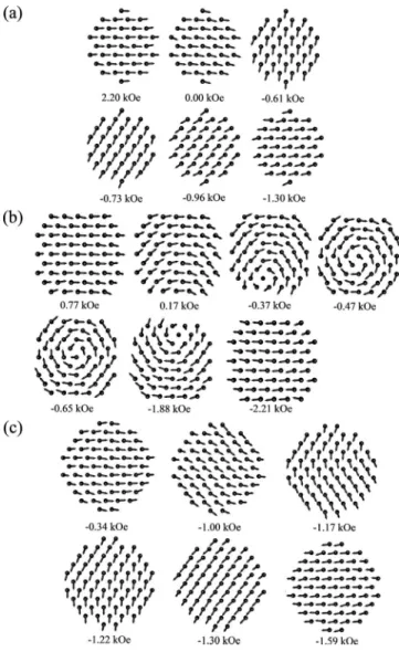
(4) PHYSICAL REVIEW B 81, 184417 共2010兲. MEJÍA-LÓPEZ et al.. FIG. 4. 共Color online兲 Ratio of the loop width at coercivity to the width at half saturation for a 65 nm diameter dot as a function of number of MCS.. mental results is obtained. Then, the number of MCS is kept fixed and all other variables are modified. Hence, we first study the effect of the number of MCS on ␦. Figure 4 illustrates ␦ for a 65-nm-diameter dot as a function of the number of MCS. ␦ asymptotically converges to 0.35 for 2400 MCS per field value. However, the effects discussed here are weakly dependent on the MCS for MCSⱖ 600. In the simulation, the magnetization curve is started at H = 2.6 kOe applied along the 关100兴 crystallographic direction, labeled the x axis, with the initial configuration in which most of the magnetic moments point along this direction. We define M s as the magnetization at the maximum applied field 共2.6 kOe兲, M r—the remanent magnetization, and Hc—the coercivity. Field steps of ⌬H = 10 Oe are used in all calculations. Typically, we perform 6.24⫻ 106 Monte Carlo steps per spin for a complete hysteresis loop, which is equivalent to 600 MCS per field value. Forty different seeds are used for the random number generator to improve the statistics by considering different configuration states. These 40 simulations are averaged to generate the present results. Two examples of simulated hysteresis loops are shown in Fig. 1共b兲, for the same diameters used in the experiment. The calculated loops are strongly dependent on the dot diameter and the coercivity exhibits a significant change as a function of dot size. To clarify this behavior, we investigate the magnetic configurations a dot exhibits going through its hysteresis loop, and we focus on the dependence of these magnetic configurations on the dot diameter. In general, magnetization reversal for considered here small-sized planar dots occurs by two main mechanisms, depending on the dot diameter. In the first one, known as “coherent rotation,”22 the spins follow the magnetic field orientation without formation of any complex magnetic structure inside the magnetic dot. In the second one, magnetization reversal occurs via displacement of a more complex spin structure such as a magnetic vortex, which nucleates at one side of the dot, moves across the dot, and annihilates on the other side.9 For a direct comparison to experimental observations, we study the magnetic behavior as a function of dot diameter using the same ␦ = ⌬0.0 / ⌬0.5 parameter to characterize the hysteresis 共Fig. 2兲. The zero magnetization width ␦ changes dramatically, showing a complex dependence on dot diameter. For very small dots, the ground state is a single domain. FIG. 5. Magnetic configurations during the switching process for different dot diameters: 共a兲 D = 55 nm, 共b兲 D = 65 nm, and 共c兲 D = 67 nm.. and its magnetization reverses coherently, exhibiting a hysteresis loop with a constant width,22 hence ␦ ⬇ 1. When the diameter of the dot increases, vortex nucleation drives the reversal and a “neck” is observed at zero magnetization 共see below兲. This effect is enhanced at D = 65 nm, where ␦ ⬇ 0.6. While the precise ␦ value may depend 共slightly兲 on the number of MCS 共Fig. 4兲, this “best” diameter is independent of it. A fair agreement between theoretical and experimental hysteresis loops is obtained for 600 MCS, which also provides a very good agreement between the ␦ values obtained from experiments and simulations 共Fig. 2兲. Figure 5 illustrates snapshots of the spin configurations for different values of the applied magnetic field. For dots diameters smaller than 60 nm, in all 40 simulations, these dots reverse their magnetization via the same mechanism: coherent rotation 关Fig. 5共a兲兴. From 60 to 65 nm, an increasing number of dots 共from 1 to 14兲, among the 40 seeds used, reverse their magnetization through the nucleation of a vortex, which progressively decreases ␦. For D = 65 nm, the reversal of all the dots occurs via the nucleation of a vortex state, as illustrated in Fig. 5共b兲. At this D, ␦ reaches a mini-. 184417-4.
(5) PHYSICAL REVIEW B 81, 184417 共2010兲. DEVELOPMENT OF VORTEX STATE IN CIRCULAR…. FIG. 6. 共Color online兲 Energies during the field reversal for a 60 nm 共dashed red line兲 and a 65 nm dot 共continuous blue line兲: 共a兲 total magnetic energy during the reversal, 共b兲 internal energy. Letters identify different regimes as explained in the text. Internal energy has been shifted to zero value and expressed in arbitrary units.. mum. While magnetization reversal via vortex is the only reversal mode present for 65-nm-diameter dots, for larger dots, reversal occurs both via a vortex and an S state 共coherent rotation兲 关Fig. 5共c兲兴. This leads to an increase in ␦ to almost one at D = 67 nm, where reversal occurs primarily via coherent rotation. For 67⬍ D ⬍ 80 nm, reversal for some of the dots again occurs via vortex, resulting in a new decrease in ␦. At D = 80 nm, magnetization in all the dots reverses again via vortex nucleation. It is worth noting that this does not necessarily reflect that the states via which the reversal occurs are the ground states at zero field. For most of the dot diameters above 60 nm vortex is the ground state at zero applied field. Above 65 nm, the vortex is probably unstable because the domains of out-of-plane magnetization may not be commensurate with the dot diameter, hence decreasing the gain in the total energy from nucleating a vortex.14 Figure 6 shows 共a兲 total and 共b兲 internal 共total minus Zeeman兲 energies for two dot diameters: 60 and 65 nm. In region A, all spins point along the applied field H and the internal energy remains almost constant. In region B, a small difference arises between the two dots. For D = 60 nm, the spins are aligned along the magnetic field, whereas for D = 65 nm, a so-called C state is formed. This C state is a lower energy state and therefore there is an energy decrease, 共Fig. 6兲. Region C shows an even larger difference between the two dot sizes. For the 60 nm, the energy remains almost constant although some spins start canting due to the competition between the dipolar interaction and the applied reversal field. In contrast, in the 65 nm, the formation of the vortex decreases the energy to a deep minimum, at the coercive field. This implies that a larger energy, and hence a large reversal magnetic field is needed for the magnetic configu-. ration to return to a state where all spins are lined up along the applied field, as found in region D. This explains the neck formation in the hysteresis loop. The 60 nm dots on the other hand exhibit a small minimum around −0.85 kOe due to spin canting without vortex formation. The field corresponding to this energy minimum also coincides with the coercive field. The energy barrier to come out from this canted state is much smaller than that for the vortex state. In region B, although the vortex is the ground state for the 65 nm dots,9 after in-plane saturation the dot may become stuck in the metastable C state due to the high-energy barrier between it and the vortex state. This explains the finite remanent magnetization and the nonzero coercivity. Thermal activation at higher temperatures may cause earlier vortex nucleation 共i.e., at more positive fields兲 as found experimentally.31 To calculate the core size with a reasonable precision, it is necessary to increase the number of spins considered in our simulated dot. Therefore, for this calculation we choose x = 0.00476, which gives J⬘ = 0.2, which sets N = 1332. The dot is magnetically prepared following a procedure similar to that in the neutron-scattering experiment.14 First, an external magnetic field of 3 kOe 共Hx along the +x̂ direction兲 and 34 Oe along the +ẑ direction, Hz, is applied. Then Hx is reduced in steps of 10 Oe until the magnetization becomes almost zero, in order to stabilize the vortex state. This occurs when Hx points along the negative direction of x̂. Finally, Hx is increased to zero. It is important to note that for all the calculation Hz is kept fixed. Using color coding for magnetization along the z direction, Fig. 7共a兲 illustrates the vortex-core profile obtained with these Monte Carlo simulations. The total magnetization at Hx = 0, after performing the procedure defined above, is 0.06M s. The vortex-core size Rc is calculated as in the experiment. We assume that the magnetization along the ẑ direction arises from spins totally saturated along the +ẑ direction inside a cylinder of the same height of the dot. Following these procedure, we find the vortex-core size of Rc = R冑M / M s ⬃ 16 nm in quantitative agreement with experiment. B. Analytical calculations 1. Vortex core. For an additional characterization of the vortex we employ a simplified description25,32 in which the discrete distribution of magnetic moments is replaced with a continuous ជ 共rជ兲. With this one, described by the magnetization field M ជ M 共rជ兲␦v gives the magnetic moment within the volume ␦v centered at rជ. In this, “micromagnetic” approach, the total energy 共Etot兲 of a ferromagnet is given by the sum of three terms corresponding to the magnetostatic 共Edip兲, exchange 共Eex兲, and Zeeman 共Ez兲 contributions.33 Thus, the magnetostatic term 共in Gaussian units兲 is genជ 共rជ兲 · ⵜUdv, where U共rជ兲 is the erally given by Edip = 共1 / 2兲兰M magnetostatic potential and v is the particle volume.33 Asជ 共rជ兲 varies slowly on the scale of the lattice suming that M parameter, we approximate the exchange term by Eex = A兰兺共ⵜmi兲2dv, where A is the exchange stiffness constant. 184417-5.
(6) PHYSICAL REVIEW B 81, 184417 共2010兲. MEJÍA-LÓPEZ et al.. M z共兲 have been proposed in the literature25,34,35 any value of n ⱖ 4 can approximately describe the magnetic vortexcore configuration in nanodots,25,32 provided the out-of-plane magnetization at the boundary of the core34 is small. The total energy, consisting of dipolar and exchange contributions, can be calculated analytically25,32 as given, e.g., by Eq. 共13兲 in Ref. 25 for n = 4. The total energy can be minimized with respect to the parameter B giving B / lex = 1.83 + 1.35共L / lex兲0.4. Therefore, the vortex-core magnetization 关Eq. 共4兲兴 is given by the simple expression. 再. M z共 兲 = M s 1 −. 2 0.4 −2 2 关1.83 + 1.35共L/lex兲 兴 lex. 冎. 4. 共5兲. which is independent of the dot radius, as pointed out by Shinjo et al.7 The above expression for M z共兲 is consistent with our experiments and simulations. Figure 7共b兲 shows the vortex-core profile obtained from these analytical calculations with a core radius of approximately 15 nm. This value is in agreement with our experimental and numerical results. The total magnetization produced by the core region can be obtained by integrating M z共兲 within the dot volume v, 具M z典 =. FIG. 7. 共Color online兲 Out-of-plane magnetization 共corresponding to the vortex core兲 in units of M s by using two different theoretical methods: 共a兲 Monte Carlo simulation and 共b兲 analytical calculation using Eq. 共5兲 with L = 20 nm and lex = 3.7 nm.. and mi = M i / M 0 for i = x , y , z. We recall that A is proportional to the exchange interaction energy J between the magnetic moments.33 The Zeeman term can be evaluated from ជ 共rជ兲 · H ជ dv and corresponds to the interaction of the Ez = −兰M ជ . As menmagnetization with an external magnetic field H tioned above the anisotropy 共EK兲 contribution is neglected due to the polycrystallinity of the samples. With this procedure, we obtain an analytical expressions for the energy of a noninteracting iron dot of height L and diameter D = 2R. For the vortex-core configuration, we assume that the magnetization has the functional form ˆ, M共rជ兲 = M z共兲ẑ + M 共兲. 共3兲. ˆ are unit vectors in cylindrical coordinates and where ẑ and M z and M satisfy the relation M z2 + M 2 = M s2. Thus, the profile of the vortex core is fully specified by the function M z共兲. It is worth noting that the functional form in Eq. 共3兲 does not take into account any dependence of the core shape on the coordinate z. Also it does not take account on the “halo” effect at the boundary of the core.34 We adopt a vortex-core model25,32 with a functional form M z共 兲 =. 再. 冎. M s关1 − 共/B兲2兴n for 0 ⬍ ⱕ B 0. otherwise,. 共4兲. where B ⱕ R is a parameter related to the core radius and n is a non-negative constant. Although alternative expressions for. 1 v. 冕. M z共兲dddz =. B2 Ms . 5R2. For L = 20 nm and lex = 3.7 nm we obtain B = 16.7 nm and for 2R = 65 nm we obtain 具M z典 = 0.053M s which is close to 0.06M s, obtained from our simulations. 2. Critical diameter for magnetization-reversal mode. The magnetization reversal in nanodots studied by several groups9,10,36–39 showed that for small dots the reversal occurs via coherent rotation, whereas for larger ones it is driven by nucleation, displacement, and annihilation of a single vortex, in agreement with the results discussed above. Also in Ref. 39, the authors presented a detailed phase diagram showing the critical parameters for stable and metastable spin configurations in a magnetic disk. In this section we describe briefly the crossover between coherent rotation and vortex nucleation in polycrystalline magnetic nanodots. Based on the model of Guslienko et al.10,38 for vortex nucleation, we show that below a critical size the reversal process is via coherent rotation and above it vortex nucleation appears. These mechanisms can be investigated by calculating the ជ n兲, defined as the field at corresponding nucleation field 共H which the saturated state becomes unstable and a slight change in the magnetization occurs.33 Once the nucleation field for each reversal mode is known, the critical radius at which a vortex nucleates can be obtained. To calculate the nucleation field for coherent rotation 共c兲, we consider the magnetic energy of a cylindrical dot with ជ / M s = x̂ cos + ŷ sin 兲 at uniform in-plane magnetization 共M ជ = x̂H. In the an angle with the external magnetic field H 33 continuum approach of ferromagnetism, the magnetic energy can be written in the form 共c兲 = − M sHv cos + 4 M s2v共1 − Nz兲/4, Etot. where the first term corresponds to the Zeeman energy and the second one is the dipolar contribution with Nz the demag-. 184417-6.
(7) PHYSICAL REVIEW B 81, 184417 共2010兲. DEVELOPMENT OF VORTEX STATE IN CIRCULAR…. netizing factor. If H ⬎ 0, the energy minimum occurs at = 0, corresponding to the magnetization aligned with the applied field. The nucleation field for coherent rotation 共H共c兲 n 兲 can be obtained as the value of the external field at which 共2E共c兲 / 2兲=0 = 0, giving H共c兲 n = 0. 10,38 The vortex nucleation field 共H共v兲 n 兲 has the form 2 2 H共v兲 n = 4 M s关F共L/R兲 − 4lex/R 兴,. 共6兲. where lex = 共2A / 4 M s2兲1/2 is the exchange length, R is the radius, and L is the thickness. The function F共L / R兲 is given by F共兲 = F1共兲 − F2共兲 with10 F 共  兲 =. 冕 冋 ⬁. 0. 册. 1 − e −t 2 dt 1− J共t兲. t t. 共7兲. 共c兲 Thus, by solving H共v兲 n = Hn we can extract information about the critical size for magnetization reversal via coherent rotation and nucleation of a single vortex. Therefore the critical size is given by the relation 2 F共L/Rn兲R2n = 4lex ,. 共8兲. where we define Rn as the dot radius such that the nucleation fields for coherent rotation and vortex nucleation are the same. As the nanodots investigated in this paper have the radius larger than their thickness, that is L / R ⬍ 1, we can approximate F共q兲 by a simple expression F共q兲 ⬇ 0.11q − 0.022q2, and Eq. 共8兲 can be expressed as 2 Rn ⬇ 0.2L + 36.6lex /L,. tometry, neutron scattering, numerical simulations, and analytical calculations. This comprehensive study implies that the magnetic reversal for dots smaller than 60 nm occurs via single-domain state, which is also the ground state at zero field. Their reversal results in the hysteresis loops with parallel branches. When the dot diameter becomes larger than 60 nm, magnetic reversal occurs via nucleation of a vortex which is also the ground state for 65 nm Fe nanodots at zero field. This reversal is accompanied by the hysteresis loops with a neck close to zero magnetization. The hysteresis loop shape is characterized by introducing a parameter ␦, which measures the ratio of the width of the hysteresis loop at M = 0 共zero magnetization兲 and that at M = 0.5M s. Using this parameter, we classify different magnetic states as function of dot diameter. In particular, we observe that this parameter is close to one when reversal occurs as a single domain, while it becomes less than one for the vortex state. We find an excellent agreement of the size dependence of this parameter between Monte Carlo simulations and experimental measurements. For the vortex state, a vortex core, the region with out-ofplane magnetization, appears. Neutron scattering, numerical simulation, and analytic calculations find a core diameter of 16–19 nm for the 65 nm magnetic dots.14 Monte Carlo simulations and analytical calculations of the vortex core are consistent with a circular Gaussian shape of the core.. 共9兲. Therefore, provided the dot thickness L and exchange length lex are known, we can estimate Rn from Eq. 共9兲. For R ⬍ Rn we can expect that coherent rotation takes places, whereas for R ⬎ Rn we can expect that the reversal occurs by nucleation of a single vortex. The above expression 关Eq. 共9兲兴 gives insight into the complicated shape of the parameter ␦ depicted in Fig. 2. As mentioned earlier, for iron nanodots with L = 20 nm, coherent rotation 共hysteresis loops with ␦ ⬇ 1兲 for dots with D ⱗ 60 nm appears, whereas for larger diameters 共60–65 nm兲, an increasing number of dots reverse their magnetization through the nucleation of a vortex, and then ␦ decreases. The critical diameter at which ␦ starts deviating from 1 can be interpreted as 2Rn. For the parameters used in this paper, L ⬇ 20 nm and lex ⬇ 3.7 nm, we obtain 2Rn ⬇ 58 nm in good agreement with the experiments as well as with the Monte Carlo simulations, which averages over a large number of noninteracting nanodots. IV. CONCLUSIONS. We report on the dependence of the magnetic state of Fe magnetic nanodots on their diameter, studied with magne-. ACKNOWLEDGMENTS. J.M.L., D.A., J.E., and P.L. acknowledge support from AFOSR, FONDECYT under Grants No. 1050066, No. 1080300, No. 11070010, and No. 11080246, the Millennium Science Nucleus “Basic and Applied Magnetism” Grant No. P06-022-F, Financiamiento Basal para Centros Científicos y Tecnológicos de Excelencia, and the program “Bicentenario en Ciencia y Tecnología” PBCT under Project No. PSD-031. J.M.L. acknowledges support from Vicerrectoría Adjunta de Investigación y Doctorado-PUC under Proyecto Límite No. 06/2009. A.H.R. acknowledges support from CONACyT Mexico under Project No. J-59853-F. I.V.R. acknowledges support from Texas A&M University. I.V.R. and A.H.R acknowledge support from Texas A&M University— CONACyT Collaborative Research Grant Program. X.B. acknowledges the financial support of the Spanish MICINN 共Grant No. MAT2009-08667兲, Catalan DIUE 共Grant No. 2009SGR856兲 and University of Barcelona 共International Cooperation兲. We acknowledge the computer resources from CNS IPICYT, Mexico. Research at UCSD was supported by AFOSR and DOE.. 184417-7.
(8) PHYSICAL REVIEW B 81, 184417 共2010兲. MEJÍA-LÓPEZ et al. 1. J. I. Martín, J. Nogues, K. Liu, J. L. Vicent, and I. K. Schuller, J. Magn. Magn. Mater. 256, 449 共2003兲. 2 Y. B. Gaididei, V. P. Kravchuk, D. D. Sheka, and F. G. Mertens, Low Temp. Phys. 34, 528 共2008兲. 3 J. M. Shaw, S. E. Russek, T. Thomson, M. J. Donahue, B. D. Terris, O. Hellwig, E. Dobisz, and M. L. Schneider, Phys. Rev. B 78, 024414 共2008兲. 4 H. Shinohara, M. Fukuhara, T. Hirasawa, J. Mizuno, and S. Shoji, J. Photopolym. Sci. Technol. 21, 591 共2008兲. 5 C. Nam, Y. S. Kim, W. B. Kim, and B. K. Cho, Nanotechnology 19, 475703 共2008兲. 6 S. Okamoto, N. Nikuchi, T. Kato, O. Kitakami, K. Mitsuzuka, T. Shimatsu, H. Muraoka, H. Aoi, and J. C. Lodder, J. Magn. Magn. Mater. 320, 2874 共2008兲. 7 T. Shinjo, T. Okuno, R. Hassdorf, K. Shigeto, and T. Ono, Science 289, 930 共2000兲. 8 S.-B. Choe, Y. Acremann, A. Scholl, A. Bauer, A. Doran, J. Stöhr, and H. A. Padmore, Science 304, 420 共2004兲. 9 J. Mejía-López, D. Altbir, A. H. Romero, X. Batlle, I. V. Roshchin, C.-P. Li, and I. K. Schuller, J. Appl. Phys. 100, 104319 共2006兲. 10 K. Yu. Guslienko, V. Novosad, Y. Otani, H. Shima, and K. Fukamichi, Phys. Rev. B 65, 024414 共2001兲. 11 A. Hubert and R. Schafer, Magnetic Domains 共Springer-Verlag, Berlin, 2000兲. 12 J. P. Park and P. A. Crowell, Phys. Rev. Lett. 95, 167201 共2005兲. 13 X. M. Cheng, K. S. Buchanan, R. Divan, K. Y. Guslienko, and D. J. Keavney, Phys. Rev. B 79, 172411 共2009兲. 14 I. V. Roshchin, C.-P. Li, H. Suhl, X. Batlle, S. Roy, S. Sinha, M. R. Fitzsimmons, J. Mejía-López, D. Altbir, A. H. Romero, and I. K. Schuller, EPL 86, 67008 共2009兲. 15 J. d’Albuquerque e Castro, D. Altbir, J. C. Retamal, and P. Vargas, Phys. Rev. Lett. 88, 237202 共2002兲. 16 P. Vargas, D. Altbir and J. d’Albuquerque e Castro, Phys. Rev. B 73, 092417 共2006兲. 17 W. Zhang, R. Singh, N. Bray-Ali, and S. Haas, Phys. Rev. B 77, 144428 共2008兲. 18 J. Mejía-López, P. Soto, and D. Altbir, Phys. Rev. B 71, 104422 共2005兲. 19 C.-P. Li, I. V. Roshchin, X. Batlle, M. Viret, F. Ott, and I. K.. Schuller, J. Appl. Phys. 100, 074318 共2006兲. Masuda and S. Masahiro, Jpn. J. Appl. Phys., Part 2 35, L126 共1996兲. 21 The domain-wall width, 共A / K兲1/2, in Fe is estimated to be about 60 nm. 22 E. C. Stoner and E. P. Wohlfarth, Philos. Trans. R. Soc. London, Ser. A 240, 599 共1948兲. 23 R. K. Dumas, C.-P. Li, I. V. Roshchin, I. K. Schuller, and K. Liu, Phys. Rev. B 75, 134405 共2007兲. 24 The out-of-plane field is needed to maintain the polarization of the neutron beam and to set the direction of the vortex-core magnetization 共“vortex polarity”兲. 25 D. Altbir, J. Escrig, P. Landeros, F. S. Amaral, and M. Bahiana, Nanotechnology 18, 485707 共2007兲. 26 C. A. Ross, M. Farhoud, M. Hwang, H. I. Smith, M. Redjdal, and F. B. Humphrey, J. Appl. Phys. 89, 1310 共2001兲. 27 M. Grimsditch, Y. Jaccard, and I. K. Schuller, Phys. Rev. B 58, 11539 共1998兲. 28 C. Kittel, Introduction to Solid State Physics, 6th ed. 共Wiley, New York, 1986兲. 29 K. Binder, Rep. Prog. Phys. 60, 487 共1997兲. 30 E. De Biasi, C. A. Ramos, R. D. Zysler, and H. Romero, Phys. Rev. B 65, 144416 共2002兲. 31 R. K. Dumas, C.-P. Li, I. V. Roshchin, I. K. Schuller, and K. Liu, Appl. Phys. Lett. 91, 202501 共2007兲. 32 P. Landeros, J. Escrig, D. Altbir, D. Laroze, J. d’Albuquerque e Castro, and P. Vargas, Phys. Rev. B 71, 094435 共2005兲. 33 A. Aharoni, Introduction to the Theory of Ferromagnetism 共Clarendon Press, Oxford, 1996兲. 34 R. Höllinger, A. Killinger, and U. Krey, J. Magn. Magn. Mater. 261, 178 共2003兲. 35 See, e.g., N. A. Usov and S. E. Peschany, J. Magn. Magn. Mater. 118, L290 共1993兲. 36 R. P. Cowburn, D. K. Koltsov, A. O. Adeyeye, M. E. Welland, and D. M. Tricker, Phys. Rev. Lett. 83, 1042 共1999兲. 37 M. Schneider, H. Hoffmann, and J. Zweck, Appl. Phys. Lett. 77, 2909 共2000兲. 38 K. Yu. Guslienko and K. L. Metlov, Phys. Rev. B 63, 100403共R兲 共2001兲. 39 S. Savel’ev and F. Nori, Phys. Rev. B 70, 214415 共2004兲. 20 H.. 184417-8.
(9)
Figure

Documento similar
