A method for ion phase space validation for below therapeutic ion fluences (by single ion tracking)

Texto completo

(1)Physics Institute, Pontificia Universidad Católica de Chile Medicine Faculty, Heidelberg University. A method for ion phase space validation for below therapeutic ion fluences (by single ion tracking) Marcos Ali Vásquez Reyes. A thesis submitted in the fulfillment of the requirements for the degree of Master in Clinical Medical Physics. Supervisor:. Dr. Mária Martišíková. Co-supervisor: Dr. Paola Caprile. September 2018.

(2) ABSTRACT A wide-spreading technique for treating cancer patients in developed countries is ion beam radiation therapy. This is due to the advantageous dose deposition pattern of ions and to their radiobiological effects in tissue. The dose calculation procedure for the treatment planning of this kind of therapy requires a facility-specific ion beam model. A phase space of the particles leaving the beamline represents an alternative to the simulation of the complete beamline. In experiments with the silicon pixelated detector TimePix, 2-3 orders of magnitude of lower fluences than therapeutic ones are required, so the detector is not saturated. A method for assessing the validity of the therapeutic phase spaces under low fluence operation was developed in this thesis. The investigation included proton, helium, and carbon ion beams, using a phantom-free tracking system. This system was composed of two TimePix detectors. Measured and simulated primary ion track distributions were compared based on the width of their angular distributions. In general, wider angular distributions were obtained for the measured primary tracks than in the Monte Carlo simulations with pregenerated phase space files considering a continuous detector. The narrower the beam, the larger the obtained differences between measured and simulated width of the angular distributions. Above the limit of the angular resolution of the tracker (0.84°), the measured difference to Monte Carlo calculations was above 2.1%. In the future, an improved angular resolution of the tracking system and an improved alignment procedure are needed to make a final statement about the accuracy of the phase space files in the low fluence range for the whole span of available beam widths. This work establishes a methodology for a track-based comparison between Monte Carlo simulations and measurements using single-ion tracking.. i.

(3) LIST OF CONTENTS Abstract …………………………………………...……………………………….. i. 1. Introduction ……………………………………………………………………... 1. 2. Background ……………………………………………………………………... 4. 2.1 Radiation in medicine .…………………..……………..…………..... 4. 2.1.1 Ion beam radiotherapy ……………………………………... 5. 2.2 Interaction of therapeutic ions with matter …………………………. 6. 2.2.1 Energy loss ..………………………….………..……………. 6. 2.2.2 Absorbed dose and the Bragg curve ………..................... 7. 2.2.3 Multiple Coulomb Scattering ………………………………... 9. 2.2.4 Radiobiological aspects of ion beam hhhhhhhhhhhhhhhhhhhhh hhhhhhhhhhhhhh. radiation therapy ……………………………………………… 11 3. Material and methods ……………………………………………………………. 15. 3.1 Experimental materials ………………………………………………... 15. 3.1.1 Heidelberg Ion Beam Therapy Center ……………............. 15. 3.1.2 TimePix detector: design & operation modes .................... 17. 3.1.3 Charge sharing effect: formation of the clusters ................ 19. 3.1.4 Experiments …….…………………………………………….. 21. 3.2 Analysis of the experimental data …………………………………….. 22. 3.2.1 Cluster refinement process ………………………………....... 22. 3.2.2 Particle tracking ……………………………………………….. 24. 3.2.3 Alignment of the tracking system based on a low fluence rate …..………..……………….....……... ii. 26.

(4) 3.2.4 Alignment of the tracking system based on a therapeutic fluence rate ………………………………. 27. 3.2.5 Angular resolution of the tracker .…………………………. 28. 3.3 Monte Carlo code FLUKA …………………………………………….. 29. 3.3.1 Modelling the beam source using phase space files …………………..…………………………... 30. 3.3.2 Geometry definition……………………………………………. 31. 3.3.3 Information scoring…………………………………………….. 32. 4. Results …………………………………………………………………………….. 34. 4.1 Alignment of the tracking system ………………………………………. 34. 4.1.1 Low fluence approach ……………………………………….. 34. 4.1.2 Therapeutic fluence approach ………………………………. 42. 4.2 Cluster refinement process ……………………………………………. 44. 4.3 Angular distributions of the particle tracks ……..……………………. 47. 5. Discussion and Outlook …………………………………………………………. 53. 5.1 Alignment of the tracking system ……………………………………... 53. 5.2 Analysis of cluster properties……………………………………………. 55. 5.3 Analysis of the tracks ………………………………………………….. 56. 5.4 Evaluation of the phase space………………………………………... 58. 5.5 Outlook …………………………………………………………………... 58. 6. Summary and Conclusions ……………………………………………………... 60. References …………………………………………………………………………... 62. iii.

(5) To my beloved O.P.P..

(6) Chapter 1: Introduction. 1 INTRODUCTION As published recently by the World Health Organization [1], cancer is the second leading cause of death worldwide. It was estimated that during 2015 there were 8.8 million deaths related to this disease, this is 1 out of 6 deaths were cancer associated. It was found that tobacco use is the main risk factor, since 22% of the analyzed cancer deaths were caused by smoking [2]. Regarding the global leading cancer malignancies causing patient death, lung cancer is above all the other cancer types, followed by liver, colorectal and breast malignancies [1]. As reported by Stewart et al [3] five major approaches are being used as cancer treatment strategies: surgery, radiation, drug therapy, integrative medicine and palliative care. The decision of which treatment approach to implement is determined by multiple factors, namely: cancer type and progression, patient specific biological factors (e.g. genes mutation) and the tissue or organ where the cancer was originated. With respect to radiation treatment, different techniques are available nowadays. For example, external beam radiotherapy with photons or charged particles, and brachytherapy. However, this work is focused on external radiotherapy, specifically with ion beams (IBRT). This technique was firstly proposed by Robert Wilson in 1946 [4] and 8 years later the first proton treatment was performed on a human pituitary gland [5]. Two main advantages can be recognized in IBRT: the first is related to the way ions deposit energy in depth and the second is the radiobiological effect of ion irradiation in tissue. The ions energy-deposition is determined by the characteristic Bragg curve, enabling to reach lower entrance dose, while the maximum energy deposition is located in the target. This IBRT property leads to a better dose conformity to the target than the one achieved with photons. As a result, higher doses can be delivered 1.

(7) Chapter 1: Introduction. to the tumor volume leading to an increased tumor control probability (TCP) while maintaining the normal tissue complication probability (NTCP) within tolerance values. In order to obtain a full dose coverage of the tumor volume several ion beam energies must be used, resulting in a superposition of Bragg peaks which has been named spread out Bragg peak (SOBP). As IBRT treatments must be delivered very accurately due to the potential biological effects [6], the treatment planning process includes a dose calculation procedure. For this purpose, Monte Carlo simulations has been shown to increase the accuracy of the dose computation [7] in comparison to other techniques as pencil beam, convolution or superposition. At the Heidelberg Ion Beam Therapy Center (HIT- Heidelberg, Germany), IBRT treatments have been implemented since 2009. One of the used techniques for IBRT is the active beam delivery system. This system is based on the magnetic deflection of narrow beams (pencil beams) by means of dipole magnets (horizontally and vertically located) through the target volume. In this raster scan delivery mode, the location of the beam spot as well as the initial energy of the incoming particles is varied to fully cover the tumor volume. The available width of the beams is in the range between 4 to 10 mm full width at half maximum (FWHM), according to the ion specie and initial beam energy. In a treatment plan field around 50000 individual beam spots with approximately 50 different beam primary energies are used [8]. In order to provide facility-specific beam model at HIT, a FLUKA-based Monte Carlo simulation of the beam nozzle was performed [9] for the different ion types, beam energies and foci available at this facility, containing primary and secondary particles information such as energy, mass and cosine direction along the beam path. This information is stored in the so-called phase space files, and can be more easily used by external facility users for setup-specific simulations. The aim of this thesis was to develop a methodology to assess the accuracy of the phase space by comparing Monte Carlo simulations using phase space files and experimental data in terms of single ion tracking. The research was performed for proton, helium and carbon ion beams, each at the lowest, middle and largest beam 2.

(8) Chapter 1: Introduction. energy offered. The largest available pencil beam width was investigated using a phantom-free setup including a tracking system. The system was composed of two pixelated silicon detectors (TimePix) developed at the European Organization for Nuclear Research (CERN), each with a sensitive area of 2 cm2. All the measurements were performed in the experimental beamline of the HIT. The content of this thesis is the following: Chapter 2 describes the physical background of this thesis, Chapter 3 introduces the material and methods used during the reported research, Chapter 4 shows the main results, Chapter 5 provides discussion and outlook and Chapter 6 contains summary and conclusion.. 3.

(9) Chapter 2: Background. 2 BACKGROUND. T. heoretical principles behind radiation in medicine, more specifically ion beams, are addressed in this chapter, which is divided in two sections. Section 2.1 presents why ion beam radiation is advantageous for cancer treatment. In section 2.2 interactions of heavy ions with matter are summarized, as well as the main. radiobiological properties of ions.. 2.1 Radiation in medicine People are naturally exposed to low doses of high-energy radiation coming from the space, and the earth [10], as depicted in Figure 2.1. This high-energy radiation is called ionizing radiation since it is able to ionize matter while passing through. Due to this property, ionizing radiation is able to produce damage to biological systems but at the same time it can be used in such a way that great benefits are obtained. In the medical area, ionizing radiation is applied for the diagnosis of many diseases and to treat some malignancies.. Figure 2.1 Approximated distribution of radiation exposure (reprinted from [10]).. With regard to the treatment of malignancies, ionizing radiation represents a powerful mean to destroy tumor cells by causing damage to the genetic material of the cell (DNA) located in its nucleus. The damage to the DNA aims to produce cancer cell death, 4.

(10) Chapter 2: Background. stopping in this way its proliferation. This can be achieved, since tumor cells show noneffective damage repair mechanisms. In order to deliver radiation to tumors two methods can be applied [11]: . External Beam Radiation Therapy (EBRT): is delivered from outside the body by directing high-energy rays (photons, electrons, protons, neutrons or heavier ions) to the location of the tumor. This is the most common approach in the clinical setting.. . Internal Radiation or Brachytherapy (BRT): is delivered from inside the body (or on the surface of the body) using radioactive sources.. Moreover, combined treatment modalities are also possible. When used before surgery (neoadjuvant therapy), radiation aims to shrink the tumor to facilitate its resection while if used after surgery (adjuvant therapy), radiation aims to destroy microscopic tumor cells that may have been left behind [11].. 2.1.1 Ion beam radiotherapy Ion beams are created when ions are accelerated [12]. The use of ion beams is vast. They have been widely used in science and the industry, mostly for spectroscopy or surface analysis and modification [13], but also in the medical field as a cancer treatment. For this aim the mostly used ions are the lightest hydrogen ions (protons), followed by carbon, while others as helium and oxygen are still in the research phase. One of the crucial persons in the field of ion beam therapy and nuclear medicine was Ernest Lawrence, inventor of the cyclotron. Together with his physician brother John, they performed a cancer therapy using artificial isotopes in 1936. Later on, they introduced the use of charged particle beams for therapy [14]. Nowadays technology enables to accelerate ions to precisely calculated energies and to target them towards tumor cells with high accuracy [14]. Due to the proven advantages of particle therapy over photon therapy, interest in ion beams has increased. Up to now, Austria (MedAustron), Italy (National Center of Oncological Hadrontherapy), China (Shanghai Proton and Heavy Ion Center), Japan (Heavy Ion Medical Accelerator in. 5.

(11) Chapter 2: Background. Chiba) and Germany (Heidelberg Ion Beam Therapy Center) own facilities offering heavy ion therapy [15]. By the end of 2016, patients around the world who benefit from particle therapy with protons accounted for 149,345 while about 21,580 patients received carbon ion radiotherapy [16]. The main indications for ion beam RT include [17]: . Skull-base tumors. . Head and neck tumors. . Prostate. . Hepatocellular Carcinoma (HCC). . Bone and soft tissue sarcomas. . Non-small cell lung cancer (NSCLC). . Recurrent rectal cancer. 2.2 Interaction of therapeutic ions with matter In this section main interactions of therapeutic ion beams are addressed, namely: the energy loss of charged particles passing through a medium, the Bragg curve, Multiple Coulomb scattering and finally the biological effect of IBRT.. 2.2.1 Energy loss When a charged particle passes through a medium, it loses its kinetic energy by mainly transferring it to the electrons of the traversed material. Ionization of matter has numerous applications, for instance, in developing detectors for particle and nuclear physics or in defining protection regulations against radioactivity. In order to calculate the rate of energy loss of an ion in matter the following formula by Hans Bethe and Felix Bloch [18] can be applied:. 𝑑𝐸 4𝜋𝐾 2 𝑍 2 𝑒 4 𝑁 2𝑚𝑒 𝑐 2 𝛽 2 𝛿 2 − = (𝑙𝑛 ( ) − 𝛽 − ) 𝑑𝑥 𝑚𝑒 𝑐 2 𝛽 2 𝐼(1 − 𝛽 2 ) 2 6. (2.1).

(12) Chapter 2: Background. where β=v/c, c is the speed of light, Z is the atomic number, e is the electron charge, me is the electron rest mass, K is a constant, N is the number density of atoms in the medium and I is the mean excitation energy of the medium. The minus sign on the left-hand side in equation 2.1 is simply a reminder that the formula gives the energy lost by the particle [19]. Due to the factor 1/β2 the highest energy deposit rate is localized in a region near the stopping point of the charged particle [18]. The last term in equation 2.1 is a correction for the so-called density effect. The determination of the mean excitation energy is normally an empirical task. However the International Commission on Radiation Units and Measurements (ICRU) in its report 37 has provided some estimates based on experimental stopping-power measurements for protons, deuterons, and alpha particles which is shown in Figure 2.2:. Figure 2.2 Estimates of mean excitation energy provided in the ICRU report 37 depicted as a curve. Reprinted from [20].. 2.2.2 Absorbed dose and the Bragg curve In radiotherapy the most important physical quantity is the dose absorbed in tissue [21]. It is defined in the ICRU as the mean energy 𝑑𝜖̅ deposited by ionizing radiation in a mass element 𝑑𝑚: 𝐷=. 𝑑𝜖̅ 𝑑𝑚 7. (2.2).

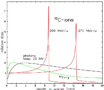
(13) Chapter 2: Background. The unit of absorbed dose is the Gray: 1 𝐺𝑦 = 1. 𝐽 𝑘𝑔. (2.3). The quantity absorbed dose represented in equation 2.2 is non-stochastic and it is defined in a material of mass density ρ (in RT water is the reference material) over an infinitesimal volume dV at a point of interest during a certain period of time [21]. Photons and ions have a very different depth-dose profile due to the different mechanisms that govern their interactions with matter. The depth dose profiles of protons and other ions like helium and carbon show the maximum dose deposition at the end of their path in tissue (as described by equation 2.1) and a low dose along the entrance of the beam. Photons exhibit their maximum near the surface and as a consequence high doses are deposited in the entrance for a single beam. The maximum of an ion depth dose profile has been called the Bragg peak and its location can be varied by changing the beam energy, as shown in Figure 2.3. In this figure it can be seen that as energy increases, ions can travel further in water and therefore the Bragg peak will be located deeper. This characteristic has been exploited clinically, by irradiating very deep-sited tumors with high doses while minimizing the delivered dose to organs at risk.. Figure 2.3 Comparison of depth dose profiles produced by electromagnetic radiation (from 60-Co and linac) and carbon ions of two different energies in water. The characteristic Bragg peak located at different depths can be observed. Reprinted from [21]. 8.

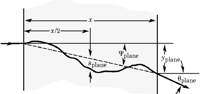
(14) Chapter 2: Background. When Bragg peak curves produced by protons and heavier ions are compared, it is possible to distinguish a dose tail behind the Bragg peak. This tail is produced by the fragmentation of heavy ions, as shown in Figure 2.4. These fragmentation processes take place through nuclear reactions [22].. Fragmentation tail. Figure 2.4 Comparison of a proton and a carbon Bragg peak curve in water, where the presence of the fragmentation dose tail is shown. Reprinted from [22].. Protons and heavier ions differ in two main radiobiological and physical characteristics [22]: . Protons have a similar biological effect as photons for the same absorbed dose, while heavy ions show a varying Relative Biological Effectiveness (RBE) ranging from low values in the plateau region to a significant enhancement in the Bragg peak.. . As depicted in the figure above, heavy ions exhibit a characteristic dose tail behind the Bragg peak.. 2.2.3 Multiple Coulomb scattering When a charged particle traverses a medium, its trajectory can be affected by small angle deflections produced by the interactions with the surrounding nuclei [28]. The change in the trajectory of the projectile is exemplified in Figure 2.5.. 9.

(15) Chapter 2: Background. Figure 2.5 Due to multiple Coulomb scattering (MCS) a charged particle deviates from a straight trajectory while traversing a medium. Reprinted from [20].. There are several applications in which multiple scattering of charged particles is of interest. Applications are related to directed-beam ion transport codes and the simulation of the physical and biological dose [23], among others. Therefore, if an accurate theory that models MCS is applied, the precision of experiments and simulations related to fast charged particles will be improved [24]. For this thesis, MCS is important since it may produce angular distributions broadening of the particle tracks in the investigated ions. In this context, it is expected that scattering is more predominant for light ions (hydrogen and helium) than for carbon ions. Multiple scattering is well described by the Moliere theory [25], nevertheless further corrections were added by Bethe [26] and Fano [27]. Even though in Moliere theory, inelastic collisions with atomic electrons are not taken into account, they may also contribute to multiple scattering. For inelastic collisions of incident heavy particles, small angle deflections take place [29]. For small angle deflections the Coulomb scattering distribution is Gaussian-like with a width given by [20]:. 10.

(16) Chapter 2: Background. 𝜃0 =. 13.6 𝑀𝑒𝑉 𝑧√𝑥/𝑋0 [1 + 0.038ln(𝑥/𝑋0 )] 𝛽𝑐𝑝. (2.4). where βc is the velocity, p is the momentum and z is the charge number of the projectile and x/X0 is the thickness of the traversed material in radiation lengths. If large angle deflections occur, a Gaussian distribution is no longer appropriate to describe multiple scattering since it starts showing a Rutherford-like scattering. Considering x and y axes to be perpendicular to the direction of the motion of the charged particle the nonprojected (in space) and projected (in a plane) angular distributions are respectively [20]: 𝑑𝜃𝑠𝑝𝑎𝑐𝑒 ≈. 2 𝜃𝑠𝑝𝑎𝑐𝑒 1 𝑒𝑥𝑝 (− ) 𝑑𝛺 2𝜋𝜃02 2𝜃02. 1. 𝑑𝜃𝑝𝑙𝑎𝑛𝑒 ≈. √2𝜋𝜃0. 𝑒𝑥𝑝 (−. 2 𝜃𝑝𝑙𝑎𝑛𝑒. 2𝜃02. (2.5). ) 𝑑𝜃𝑝𝑙𝑎𝑛𝑒. (2.6). where θ is the deflection angle and 2 2 2 𝜃𝑠𝑝𝑎𝑐𝑒 ≈ (𝜃𝑝𝑙𝑎𝑛𝑒,𝑥 + 𝜃𝑝𝑙𝑎𝑛𝑒,𝑦 ). (2.7). 2.2.4 Radiobiological aspects of ion beam radiation therapy The Relative Biological Effectiveness is defined as the ratio of absorbed dose of a reference beam (predominantly 250 KV X rays, low LET) to the absorbed dose of any other radiation (high LET) to produce the same biological effect [31]. 𝑅𝐵𝐸 =. 𝐷𝑙𝑜𝑤 𝐿𝐸𝑇 𝐷ℎ𝑖𝑔ℎ 𝐿𝐸𝑇. RBE varies, among others, with: . Particle type and energy. . Dose. . Dose per fraction 11. (2.8).

(17) Chapter 2: Background. . Oxygenation. . Cell type. . Biological end point. As an example, in proton beam therapy an RBE value of 1.1 (relative to photons) is widely used for all clinical conditions [32]. However, an increase of the LET in the distal part of the Spread-Out Bragg Peak (SOBP) produces an increase of RBE variation that is not taken into account in practice [33]. This behavior results in an extension of the biologically effective range of the proton beam by ~2 mm for 160–250 MeV and ~1mm for 60–85 MeV proton beams [30]. Due to the physical properties discussed above, heavy charged particles as protons and heavier ions have been proposed to be used for medical purposes. In particular, they have been used in cancer therapy as a more effective radiation type compared with photons. In 1946 R. Wilson from Berkeley suggested the use of protons after analyzing their depth dose profile, characterized by the Bragg peak as shown in 2.2.2. Few years later, Tobias, Lawrence and Larson started treating patients with protons and then with 4He ions. Today there are around 69 centers offering proton therapy, more than 12 carbon ion accelerators dedicated to cancer treatment and 47 particle therapy centers are under construction in different countries [34]. The term Linear Energy Transfer (LET) defines the energy loss along the trajectory of the charged particle and it has been used as a parameter to describe radiobiological effects of radiation. Radiation efficiency depends on the severity of DNA damage, which in turn is related to the proximity of the DNA lesions. In comparison to the low-LET proton and photon beams, neutrons are high-LET beams. Nevertheless, carbon ions have low LET in the plateau region and high LET in the Bragg peak. The RBE and LET relation for carbon ions is depicted in Figure 2.6.. 12.

(18) Chapter 2: Background. Figure 2.6 Example of the relation between RBE and LET for carbon ions in Chinese Hamster Ovary cell line. Reprinted from [17].. As high LET radiation reduces cellular repair capacity, a potential use of this radiation type would be in the treatment of tumor cells with a high repair capacity, for example, prostate cancer. The level of oxygenation plays an important role for the effectiveness of radiation: welloxygenated cells provide a favorable environment for radiation to create potential DNA damage. Poor-oxygenated or hypoxic cells reduce the chances to kill tumor cells. This fact is shown in cell survival curves as the ones depicted in Figure 2.7. In order to quantify the oxygen effect, the concept of Oxygen Enhancement Ratio (OER) has been introduced. It is defined as: 𝑂𝐸𝑅 =. 𝐷𝑜𝑠𝑒 𝑡𝑜 𝑝𝑟𝑜𝑑𝑢𝑐𝑒 𝑎 𝑔𝑖𝑣𝑒𝑛 𝑒𝑓𝑓𝑒𝑐𝑡 𝑤𝑖𝑡ℎ𝑜𝑢𝑡 𝑜𝑥𝑦𝑔𝑒𝑛 𝐷𝑜𝑠𝑒 𝑡𝑜 𝑝𝑟𝑜𝑑𝑢𝑐𝑒 𝑡ℎ𝑒 𝑠𝑎𝑚𝑒 𝑒𝑓𝑓𝑒𝑐𝑡 𝑤𝑖𝑡ℎ 𝑜𝑥𝑦𝑔𝑒𝑛. (2.9). In relation to the effect of the level of oxygenation in radiation therapy, the following observations have been made [30]:.  Hypoxic cells are present in most malignant tumors.  Hypoxic cells are about 3 times more radioresistant than cells with normal levels of oxygen when exposed to low LET radiations. The presence of even a small 13.

(19) Chapter 2: Background. percentage of hypoxic cells (1% down to 0.1%) can make the tumor resistant to radiation therapy..  OER decreases when LET increases, meaning that the effect of hypoxic cells in controlling tumor response will be much less for high LET radiations. Generally, the OER has a value ranging between 2.5 and 3.0 for large single doses of X or gamma rays, between 1.5 and 2.0 for radiations of intermediate LET, and 1.0 for high LET radiations, meaning there is no oxygen effect [35].. Figure 2.7 Surviving fractions of Human Kidney Cells irradiated under hypoxic and normoxic conditions with three different radiation types of increasing LET: photons, neutrons and alpha particles. Reprinted from [30].. 14.

(20) Chapter 3: Material and methods. 3 MATERIAL AND METHODS n this chapter a description of the used devices during measurements and the different. I. mathematical tools implemented during this work are addressed. Section 3.1 shows information regarding the experiments carried out. Section 3.2 introduces the analysis of the experimental data regarding the cluster refinement process and matching. procedure, particle tracking, the alignment of the tracking system based on low fluence range and a therapeutic fluence range, and the angular resolution of the tracker. In addition, section 3.3 presents information concerning the Monte Carlo FLUKA code and the phase space files used to simulate the ion beams.. 3.1 Experimental materials In this section information in relation to the performed experiment during this work is presented, namely: the HIT facility, the TimePix detector, the experimental set up and measurement parameters.. 3.1.1 Heidelberg Ion Beam Therapy Center The Heidelberg Ion Beam Therapy Center is the result of a project started in 1994 by the Society for Heavy Ion Research (GSI: Gesellschaft für Schwerionenforschung), the German Cancer Research Center (DKFZ: Deutsches Krebsforschungszentrum) and the Heidelberg University Hospital [36]. The first preparational stage of the project ended in 1997 with the first patient treated with carbon-ion therapy in Germany, implementing an active beam application at the GSI [37]. Around 440 patients were treated during the 19972008 period. Three years after the successful first treatment, the collaboration started a study regarding the feasibility of a dedicated facility based on a linear acceleratorsynchrotron combination. In 2004 the construction of the HIT facility started. HIT is the first dedicated ion therapy facility in Europe offering 1H and. 12C. treatments. Moreover, it. comprises the first heavy ion 360° rotating gantry worldwide. The facility treated the first patient in 2009.. 15.

(21) Chapter 3: Material and methods. At present HIT facility has 3 treatment rooms (Figure 3.1) plus an experimental/quality assurance beamline room. Two treatment rooms and the experimental one are equipped with horizontal fixed beamlines. In the third treatment room, a 670 tons heavy rotating gantry with submillimeter precision of the beam delivery [38] has been installed. Each of the treatment rooms are equipped with a raster scanning delivery system that uses narrow pencil beams. By means of a system of deflection magnets, the location of the beam can be shifted in order to cover the target volume. A Beam Application and Monitoring System (BAMS) is located just after the exit window of the vacuum tube of each beamline. The aim of the BAMS is to provide online beam analysis with regard to the ion fluence as well as the spot size and position of the beam. It consists of a pair of multiwire proportional chambers and three ionization chambers, as illustrated in Figure 3.11.. Figure 3.1 Illustration of the HIT facility. From left to right: The linear accelerator, the source of ions, the synchrotron, the two horizontal fixed beamline treatment rooms, the gantry treatment room and finally the beamline towards the QA/experimental beamline room on the very right. Reprinted from [37].. The currently available ion types at HIT are proton, helium, carbon and oxygen. However, only proton and carbon ion beams are implemented in the clinic at this moment. A selection of the initial energy of the ion beam can be done within a range of 255 predefined energy steps. In this work, the investigated ion beam types were only 1H, 4He and. 16. 12C,.

(22) Chapter 3: Material and methods. each one with the following energy steps 1, 125 and 255. Further major features and parameters of HIT may be found in Table 3.1.. Particle species Type of accelerator Beam energy Maximum beam intensity [Particles per synchrotron cycle]. Beam spot size Treatment rooms Beam delivery technique Gantry type Treatment field Number of patients per year Building area. H, He, C and O Linear accelerator plus synchrotron 48 up to 430 MeV/u 1 H: 4 X 1010 4 He: 1 X 1010 12 C: 1 X 109 16 O: 5 x 108 4-10 mm FWHM 2 horizontal fixed beamlines 1 gantry room Intensity controlled rasterscan technique 360° rotating scanning gantry, isocentrinc geometry 20 cm X 20 cm maximum >1000 Around 70 X 60 m2. Table 3.1 Technical features and working parameters of HIT. Reprinted from [36].. 3.1.2 TimePix detector: design and operation modes The TimePix radiation detector is a release of the Medipix2 Collaboration established at the European Center for Nuclear Research (CERN) in 2002, which firstly introduced the MediPix2 device [39]. As an upgrade of this detector, TimePix has similar characteristics [40] to MediPix2. These sensors are based on solid state semiconductors, in which pairs of electron and holes are created when exposed to ionizing radiation fields. Then the generated holes are collected on the readout electrodes by applying a bias voltage.. TimePix detectors have pixelated sensors, with 256 X 256 pixels distributed over a 1.4 x 1.4 cm2 sensitive area. Each pixel is 55 x 55 µm2 in size. All pixels are bump-bonded with their own electronic circuit (pre-amplifier, discriminator and digital counter) to the readout chip (Figure 3.2) by approximately 25 µm tin/lead alloy spheres. Regarding the sensor material, in this work silicon sensors were chosen together with a 300 µm thickness.. 17.

(23) Chapter 3: Material and methods. Several studies have already shown TimePix capabilities to analyze ion beam radiation fields [41-43].. Bump bonds. Figure 3.2 Left: The TimePix detector with its mother board and readout interface (FitPix). Right: Sensor´s structure, which includes the sensor chip, the bump-bond region and the readout chip. Reprinted from [44].. In the readout chip, the discriminator enables to set threshold values that can be individually defined for each pixel to enable noise-free operation. Moreover, the acquisition time (frame duration) can be defined by the user. The digital counter of each pixel is incremented according to the chosen TimePix operation mode. The modes of operation (Figure 3.3) can be chose as defined in [45]: . Counting mode: also named Medipix mode. In this operation mode the counter value increases by one every time the signal coming from the preamplifier exceeds the predefined threshold. Therefore, this mode enables to count the number of ionizing particles that impinged the sensitive area during each frame.. . Time of arrival mode (TOA): named TimePix mode too. Whenever the detector is operated in this mode, the counter starts to add one count every clock tick from the time the preamplifier output exceeds for first time the threshold value until the frame 18.

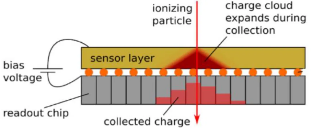
(24) Chapter 3: Material and methods. is over. This mode was used in most of the measurements performed in this study since it enables to track particles when at least two parallel detectors are operated in synchronization. . Time over threshold (TOT): known also as Energy mode. In this case the counter is continuously increasing by one count per clock tick while the preamplifier is above the predefined threshold. Due to the correlation of the time over threshold deviation and the amplitude of the collected charge in a pixel, this working mode is used to measure the deposited energy.. . Masked mode: this mode, as the name suggests, is used to mask malfunctioning pixels by disabling the counter summing up option.. Figure 3.3 Illustration of the operation principle of TimePix for the different working modes: counting, energy and time modes. When the signal exceeds the set threshold, the counter is activated. The increment of the counts vary according to the operation mode: in counting mode, the counts increase by one whenever the signal comes over the threshold. In energy mode, the counts increase as long as the signal stays above the threshold. Finally, in time mode the counts increment until the end of the frame. Reprinted from [44].. 3.1.3 Charge sharing effect: formation of the clusters An important effect occurring during measurements with TimePix is the so called charge sharing effect (Figure 3.4). Due to this effect, the charge that originally should belong to one pixel reaches neighboring pixels producing the so-called clusters. It is a consequence 19.

(25) Chapter 3: Material and methods. of the spread of the charge cloud caused by a particle that impinged the sensor. It takes place during the charge collection process. This effect has been studied by Jakubek et al [46], showing that the observed charge sharing results from electrostatic repulsion of the charge carriers and charge diffusion. Therefore its magnitude is given by the deposited energy (given the ion type/ energy) and the bias voltage. At high energy deposits, the charge sharing effect gets larger. At lower bias voltages, the charge sharing effect gets larger. In addition, in order to avoid saturation effects in the TimePix electronics, a bias voltage of 10 V was defined for all the measurements performed during the present work. As final result of the charge sharing effect, the generated cloud charge due to an impinging particle is not only collected by a single pixel, but a set of pixels that surround it. This ensemble of pixels that belong to the same particle detection event is named Cluster.. Figure 3.4 Schematic illustration of the cluster formation in which it is shown the charge sharing effect in the surrounding pixels of the impinging point. Reprinted from [46].. To characterize the clusters, the following properties can be identified: . Cluster position: this parameter is calculated as the center of mass of the cluster.. . Cluster size: number of pixels belonging to a certain cluster.. . Cluster height: maximum pixel value found inside a cluster.. . Mean cluster signal: average of the pixel values that belong to a certain cluster.. 20.

(26) Chapter 3: Material and methods. 3.1.4 Experiments In this study the experimental setup was a phantom-free tracking system. For this purpose, a set of two 300 µm thick TimePix sensors were stacked (0.36 cm distanced between each other) and assembled to a single motherboard using one readout interface. This enabled a synchronized operation of both detectors. The whole detection system was mounted on an aluminum rail and connected to a computer by means of a USB port. A remote control of the detectors was used by installing a second computer in the control room and establishing an Ethernet connection with the computer inside the room. This last computer provided with the acquisition software Pixet, was connected to the tracking system. Then the system was placed on an experimental table, located in front of the beam´s exit (nozzle), at the isocenter. The lasers installed in the room were used for positioning the detectors. The vertical laser was placed in the middle of the thickness of the first detector, the horizontal laser was placed in the middle of the sensitive area of the first detector (Figure 3.5) at a 1.1 m distance from the nozzle. A spirit level was used for achieving the parallelity with respect to the beam axis. By utilizing the Pixet software, the following acquisition parameters were set: an acquisition time of 1 ms, a counting clock with a frequency of 10 MHz, a bias voltage of 10 V and the time of arrival mode. Measurements for the validation of the phase space files were performed at HIT with the experimental beamline and selecting a low particle fluence (between a hundredth and a thousandth part of the lowest therapeutic fluence) and the largest focus available for each energy step and ion type analyzed. A first measurement dedicated to the analysis of the alignment of the tracking system was performed using 4He ion beam (low fluence) with an initial energy of 220.51 MeV/u and the smallest focus available. In a second dedicated measurement for this purpose, irradiations were performed with the lowest fluence of the therapeutic range together with the largest beam energy for this ion specie (430.10 MeV/u) and the smallest focus available.. 21.

(27) Chapter 3: Material and methods. Figure 3.5 Implemented experimental setup during this study where it can be seen how the beam is positioned in the center of sensitive area of the first detector. The beams eye view coordinate system is shown in orange arrows.. 3.2 Analysis of the experimental data This section addresses the analysis of the acquired experimental data. It includes the primary particles selection process together with the particle tracking (3.2.1, 3.1.2) and the alignment of the tracking system (3.2.3, 3.2.4). The acquired data was firstly preprocessed by C++ routines previously developed that generate files of listed clusters with the info on x and y position (center), size, and time of arrival (of the first hit pixel of the cluster) in each detector. After that, this data files were analyzed with self-written routines in Matlab 2017 b (The MathWorks, Inc., Natick, Massachusetts, United States).. 3.2.1 Cluster refinement process The cluster properties and working principle of the detection system has been already introduced in 3.1.2. Besides a correctly measured cluster, the following artifacts (depicted in Figure 3.6) can be found regarding the experimentally obtained clusters:. 22.

(28) Chapter 3: Material and methods. . Spatially cropped clusters: are the result of impinging particle positions close to the sensitive area borders (cropped orange circle in Figure 3.6). Therefore the collection is limited since no more pixels are available. The resulting cluster size can be reduced and the position not accurately measured. This effect was prevented in this work by applying a margin criteria along the border of the sensitive area, clusters between margins edges were excluded from this evaluation. For this purpose, firstly a statistical analysis was performed over the cluster radii of all recorded clusters. This radius value was obtained for each scored cluster as follows: 1 𝑟 = √ ∙ 𝐶𝑙𝑢𝑠𝑡𝑒𝑟 𝑠𝑖𝑧𝑒 𝜋. (3.1). The margin criteria was defined based on the mean cluster radius plus two standard deviations from the detector’s border. Clusters with their center of mass outside this margin were removed from the analyzed data. . Temporary cropped clusters: this kind of undesired clusters belongs to particles that impinged the sensitive layer just before the acquisition time started. Consequently their time of arrival is not correctly measured. Temporary cropped clusters have larger analog to digital counts (ADC) meaning earlier arrivals than correctly measured clusters. A constrain on the time of arrival values (cluster with TOA larger than 9990 ADC were excluded) assured that this clusters were not considered in this study.. . Overlapping clusters: which belong to clusters formed by two or more particles that impinged the TimePix detector close in space within a frame (depicted by the yellow and blue zoomed clusters in Figure 3.6). The spatially overlapping clusters have different time of arrival. Consequently a large standard deviation of the TOA values is found inside the cluster. To filter them a maximum standard deviation of the TOA within a cluster of 50 ADC was allowed.. 23.

(29) Chapter 3: Material and methods. Figure 3.6 Upper left: schematic illustration of overlapping (upper circles) and spatially cropped (orange hemi circle) clusters for a 1 ms acquisition time (frame). Color scale shows different TOA values. Upper right: cluster size spectrum showing those clusters that were rejected. Lower left: TOA spectrum in which it is indicated the region of clusters that were excluded for this study. Lower right: standard deviation spectrum of the TOA within the measured cluster. All the spectra belong to a 270.5 MeV/u carbon ion beam measurement.. 3.2.2 Particle tracking. In order to reconstruct single particle tracks from measured cluster, a matching of clusters generated by the particles was performed (Figure 3.7 –upper left panel). This process consists of the following: given a measured frame, looking for the cluster information obtained in the first sensitive layer that belongs to each detected cluster in the second sensitive layer. That is to pick information related to the same impinging particle. This was possible since Pixet software- synchronized operation was enabled. The matching task was accomplished by looking for the closest TOA of a cluster scored in detector 2 for each cluster recorded in detector 1. 24.

(30) Chapter 3: Material and methods. In this work matched clusters were considered to originate from one particle when the following criteria were fulfilled: . A maximum TOA of a cluster that belonged to the first sensitive layer had a pair in the second detector such that the difference between the maximum TOAs was smaller than 4 ADC (see distribution of difference of TOA of matched particles in Figure 3.7- lower right panel).. . The center of mass of the cluster in detector 1 had to be close to the center of mass of the cluster scored in detector 2 (less than 5 pixels). This prevented mismatching of the clusters that had similar TOA inside a frame (distribution of lateral distance between matched clusters Figure 3.7- lower left panel). By assuming forward directions of the impinging particles, they should be detected in similar positions in detector 2 with respect to the first sensor [47].. Based on the distance between detectors, if the position of the center of mass of each paired clusters is known and assuming a straight line connecting the cluster pair (blue line in Figure 3.7 upper left), the calculated angles with regard to the vector that connected the impinging position in each sensor were obtained as follows: 𝑥2 − 𝑥1 𝛼𝑥 = 𝑡𝑎𝑛−1 ( ) 𝑧2 − 𝑧1. (3.2). 𝑦2 − 𝑦1 ) 𝑧2 − 𝑧1. (3.3). 𝛼𝑦 = 𝑡𝑎𝑛−1 (. Where x, y and z are the 3D coordinates of the cluster´s center of mass in detector 1 and 2, respectively. In addition a third angle was analyzed, the so called combined angle (αcombined), since this angle already contains 3D information in comparison with the introduced αx and αy. This angle was calculate by: 𝑧2 − 𝑧1 𝛼𝑐𝑜𝑚𝑏𝑖𝑛𝑒𝑑 = 𝑐𝑜𝑠 −1 ( ) √(𝑥2 − 𝑥1 )2 + (𝑦2 − 𝑦1 )2 + (𝑧2 − 𝑧1 )2. (3.4). These angles (Figure 3.7- upper right panel) were a centerpiece of this study. The phase space validation for all the beam initial energies and ion types was based on the. 25.

(31) Chapter 3: Material and methods. comparison of the distributions of the calculated αx, αy and αcombined of primary particles. Similar particle tracking was assessed with the Monte Carlo simulations.. Figure 3.7 Upper left: schematic illustration of the matching process given a certain frame. It can be seen that the matched pair is close in x and y positions. Upper right: illustration of the calculated angles based on the impinging position in the first and second detector. Lower left: x and y lateral difference of matched clusters in raw data (same beam parameters as in Figure 3.6). Lower right: TOA difference of matched clusters in raw data.. 3.2.3 Alignment of the tracking system based on a low fluence rate An alignment of the tracking system was necessary in order to achieve highly accurate reconstruction of the particle tracks. A small misalignment between the pair of sensors may result in large track deviations. The alignment of the tracking system with respect to the beam axis was performed in a first step by positioning it according to the laser positioning system of the treatment room 26.

(32) Chapter 3: Material and methods. that offers a 1 mm precision. However, residual offsets regarding the positioning between detectors cannot be prevented by this means [48]. Further methods had to be applied in order to overcome remaining position uncertainties related to the x and y directions. As literature suggested [47-49] a dedicated measurement was performed for achieving a better precision in the alignment. In this work two approaches have been investigated using different ion fluencies and operation mode. In the low fluence approach, the TOA operation mode was chosen for both detectors. Regarding the beam parameters, the largest energy step available together with smallest focus of a 4He were selected (220.5 MeV/u and 4.9 mm FWHM focus) in order to reduce particle scattering, beam divergence and fragmentation in air [48]. In addition, a lower fluence than the therapeutic range was chosen (around a hundredth of the lowest therapeutic fluence). Single cluster positions in both detector were measured. After irradiation, a post-processing evaluation was performed based on the fluence profile scored in each detector. Four different methods were compared for this purpose, three of them based on the comparison of fluence profiles and one based on particle tracks. Each method aimed to quantify the vertical and lateral shifts to correct scored clusters position in detector 2. Further information about these methods is presented in chapter 4.. 3.2.4 Alignment of the tracking system based on a therapeutic fluence rate As in the case of the low fluence approach, the smallest focus and the largest energy step available were used. These parameters significantly reduced particle scattering, fragmentation in air and in the detectors, and beam divergence [49]. experimental setup was defined, but a. 12C. The same. ion beam with a 0.34 cm FWHM focus and. 430.1 MeV/u was chosen. Moreover, a change in the operation mode was needed since for this fluence range the counting mode was more suitable. Otherwise if selecting any other operation mode, the scored signal would always be over the threshold and this would definitely lead to a misdetection.. 27.

(33) Chapter 3: Material and methods. With these measurement parameters, smoother fluence profiles were expected. The study of the alignment of the tracking system was performed with a method based on the study of the fluence profile in each detector.. 3.2.5 Angular resolution of the tracker In an ideal case the tracker system would measure the angles of the tracks with infinite angular resolution. In that situation the measured width of the angular distributions could be directly compared to the simulated ones. The utilized detectors in the tracking system suffer of some limitations. The discrete pixels and the finite layer spacing are inherent characteristics that contribute to constrain the angular resolution of the system. Consequently, the angular resolution of the measurements were limited by the intrinsic angular resolution of the tracker. With regard to the angular resolution of a tracking system consisting of a double-layered device, the intrinsic angular resolution depends on the point resolution of the layer divided by the spacing of the detector layers (see e.g. [50]). In our case, since we had a pair of TimePix detectors with a 0.055 mm pixel size and a spacing of 3.6 mm, the intrinsic angular resolution is as follows:. 𝜎𝑖𝑛𝑡𝑟𝑖𝑛𝑠𝑖𝑐. 0.055 𝑚𝑚 √12 = √2 ∙ = 0.0062 𝑟𝑎𝑑 = 0.357° 3.6𝑐𝑚. (3.5). Where √2 considers a tracking system consisting of two detectors and √12 comes from the standard deviation of the spatial resolution assuming a rectangular distribution between [0, pitch]. Moreover, 𝐹𝑊𝐻𝑀 = 2√2 𝑙𝑛2 𝜎. (3.6). With this, we can estimate the width of the simulated distribution considering the real angular distributions (worst case- 1 pixel cluster). The corrected angular distributions FWHM, for the worst case-pixelization in which a resolution better than 1 pixel is not possible, is as follows: 𝐹𝑊𝐻𝑀𝑀𝐶 𝑝𝑖𝑥𝑒𝑙𝑖𝑧𝑎𝑡𝑖𝑜𝑛 = 𝐹𝑊𝐻𝑀𝑀𝐶 𝑐𝑜𝑛𝑡𝑖𝑛𝑢𝑜𝑠 𝑑𝑒𝑡𝑒𝑐𝑡𝑜𝑟 + 𝐹𝑊𝐻𝑀𝑖𝑛𝑡𝑟𝑖𝑛𝑠𝑖𝑐. 28. (3.7).

(34) Chapter 3: Material and methods. 3.3 Monte Carlo code FLUKA The FLUKA (FLUKtuirende KAskade) code is a general purpose Monte Carlo code that simulates the interaction and transport of hadrons, heavy ions, neutrinos, electrons and photons [51]. It was developed by the European Organization for Nuclear Research (CERN) and the Italian Institute for Nuclear Physics (INFN) [51]. The wide field of applications of this tool includes proton and electron accelerator shielding, calorimetry, dosimetry, detector design, cosmic ray physics, neutrino physics, radiotherapy, and more [52]. FLUKA was used in this study to simulate transport of the primary ion beam (proton, helium and carbon ion beams) through air and the interactions taking place in the detectors including sensitive layer, bump-bonds and readout chip. FLUKA can be stored through the graphical user interface (GUI) Flair (FLUKA advanced interface). Flair provides a user-friendly environment to create and modify FLUKA inputs, define geometry, generate executable files, compile them and finally run the simulations. All FLUKA simulations were performed using the following “cards” related to setting radiation transport parameters: . PHYSICS card: allows overriding FLUKA defaults for the following physics processesk[53]:. ▪ COALESCEnce. Activates coalescence mechanism. Coalescence is the process by which two or more particles merge during contact to form a single daughter particle.. ▪ EVAPORAT. Activates evaporation. Evaporation is a process in which the evaporative decay of produced nucleons by the irradiation of a target nucleus is analyzed. . HADROTHErapy card: this command activates the following processes with default threshold values [54]:. 29.

(35) Chapter 3: Material and methods. . EMF (ElectroMagnetic FLUKA), activates transport of photons, electrons and positrons down to 10 keV.. . *Low-energy neutron transport down to thermal energies included.. . *Ion transport threshold set at 100 keV, except for neutrons (1E-5 eV).. . *Multiple scattering threshold at minimum allowed energy.. . *Delta ray production with a 100 keV threshold.. To simulate the ion beams the phase space files from HIT [9] were used. For this, the card called SOURCE was exploited. This card allows calling user defined source routines. The phase space files will be described in 3.3.3.. 3.3.1 Modelling the beam source using phase space files In order to provide highly accurate and robust facility-specific simulations at HIT the beamline was simulated by Tessonnier et al (Figure 3.8) with the Monte Carlo code FLUKA version 2011.2c.3. It was focused on the precise model of the Beam Application and Monitoring System introduced in 3.1.1. [9]. The output of the simulations provide the HIT users accurate beam data without transferring the confidential information of the beamline and exit nozzle geometry and composition.. Figure 3.8 Schematic illustration of the two MC simulation approaches addressed in [9]. Upper image depicts a description of the modeled beamline including the BAMS. In the lower image TPSlike propagation (phase space like) in which it is consider the particle transport in vacuum until the isocenter. Reprinted from [9]. 30.

(36) Chapter 3: Material and methods. These phase spaces contain information such as charge, mass, energy, coordinates and direction cosines of each particle recorded given a certain position along the beam path [9]. The development of the phase space was based on the measurement of an infinitely narrow beam after the exit window (nozzle), with an enabled discrimination in the recorded information according to the particle type (primary or secondary particles). A very important feature of these files is that simulations using them are able to reproduce the different dose patterns from the delivery system when the respective beam scanning information is introduced. A very good agreement was found in the relative dose difference (below 0.5%) between the full modeled beamline and the phase space simulations [9]. Moreover, good agreement was found when comparing with measured data as shown in Figure 3.9.. Figure 3.9 Left: lateral dose profiles obtained by the full beamline simulation (BL) and the phase space simulations (PS) a 1H beam of 80.90 MeV/u and two different foci (F1,F4). Right: Dose profile phasespace calculated (solid line) and measured (black dots) for the same ion specie and nominal energy. Reprinted from [9].. 3.3.2 Geometry definition FLUKA implements Combinatorial Geometry (CG) to generate the required configuration representing the experimental set up. In order to create any desired geometry, basic elements called “bodies” are combined to generate “regions” to which predefined 31.

(37) Chapter 3: Material and methods. materials or compounds properties can be assigned. Examples of available bodies are planes, spheres, cones, cylinders and parallelepipeds. FLUKA enables great flexibility during geometry construction with regard to the number of possible regions (up to 10000), their size, applicable geometrical transformations such as translations and rotations and the possibility to create repetitions of a certain structure by means of the “lattice” option. In this sense it is possible to achieve great reproducibility of practically any specific geometry. To create regions the following operations can be applied to the selected bodies: union, subtraction, and intersection. Once regions have been generated a material must be assigned to them. In FLUKA every region is assigned to a homogeneous composition, either an element or a compound. FLUKA is provided with an extent list of different materials e.g. air, vacuum, water, graphite, cobalt, lead, titanium, silicon, etc., and even with 12 compounds with the recommended composition by the ICRU e.g. PMMA, bone and soft tissue among others. It is also possible to create own materials and special compounds by knowing the proportions of each component. In the FLUKA simulations both TimePix detectors were simulated in detail according to their specifications of: . Size: sensor area of 2 cm2, thickness of 300 μm, bump-bonds diameter of 25 μm, readout chip area of 2 cm2 and thickness of 100 μm.. . Composition material: sensitive layer and readout chip: silicon (Si), bump-bonds: alloy made of 63 % tin (Sn) and 37 % lead (Pb).. . Location with respect to the beam source 1.1 m (first detector) distance, and 0.36 cm with respect to each other.. For each measured ion type and energy step, 5 runs were carried out. The output of the simulations was then analyzed with regard to the angular distribution of primary particles.. 3.3.3 Information scoring In order to be able to perform the tracking, primary ions were chosen. This allowed to assume that the followed path of these particles was a straight line.. 32.

(38) Chapter 3: Material and methods. To perform the scoring of the events of interest, a modified subroutine called MGDRAW was applied. To activate the subroutine, the card USERDUMP had to be included. With this scoring option only primary ions impinging the first sensitive layer and crossing to the second sensitive layer were recorded. As a result, a file where information regarding the crossing position (x,y) in each detector was saved, together with the number of history (primary labeling).. 33.

(39) Chapter 4: Results. 4 RESULTS. T. his chapter, which is divided in three parts, summarizes the main findings of this work. The first part (section 4.1) shows the results of the alignment analysis for the tracking system based on four different methods. The second part (section 4.2) addresses the cluster properties and the effect of the cluster refinement process. Finally, in. section 4.3 the angular distributions of both, tracking experimental data and Monte Carlo simulations, are shown as the main method to validate the phase space files.. 4.1 Alignment of the tracking system As mentioned in 3.2.3, based on the assumption that the two silicon detectors are parallel and perpendicular to the beam axis, an uncertainty on the lateral or up/down misalignment that may exist between the pair of detectors remained. To overcome this issue, several studies have been done to find the shift between detectors. Thereafter the measured data (center of mass of the clusters scored in the second detector) was corrected for this error by applying the found correction factors in a linear translation. The tested approaches were dived in 2 categories: the first one using a low particle fluence approach (shown in 3.2.3) and the second which implemented a therapeutic fluence (presented in 3.2.4). In both methods the fluence spectra were determined as distributions of the center of mass of the clusters.. 4.1.1 Low fluence approach The two-dimensional and one-dimensional fluence spectra of the primary beam impinging the first detector are shown in Figure 4.1. It can be seen that there was a misalignment of the center of the tracking system with respect to the beam axis. These distributions include information of both, primary and secondary particles traversing the first sensitive layer. Since the 2D plot shows the particle fluence according to the beams eye view, the misalignment was found along the y axis with a rough value of 0.3 cm. It can be also stated by visual inspection that the beam spot is not circle-like but rather an oval shaped beam due to no isotropic fluence coming from de nozzle. The observed shape can be also 34.

(40) Chapter 4: Results. attributed to a tilted location of the tracking system with respect to the beam axis. Regarding the maximum number of detected hits in each pixel, the pixel with Pixet coordinates (189,138) was the one that was hit the most, scoring 166 hits. A total number of hits in the whole sensitive layer of 1.63 x 106 was registered. The same analysis was performed with the information acquired in the second sensitive layer with similar results to those found in detector one: the most hit pixel was that with coordinates (202,149). This pixel detected 162 impinging particles. Also it was found for this second layer a total number of hits of 1.65 x 106 in the entire detection area. Since the situation in the second detector is similar to the first one regarding the position according to the beam axis, it is not shown here.. Figure 4.1. Particle fluence profile along the x (upper) and y (lower-right) axis. 2D fluence distribution on the first detector of the tracking system (lower-left). The measurement as performed with a 220.51 MeV/u 4He beam with a nominal width 4.9 (FWHM) mm. Normalization of the integrated fluence to the maximum fluence was performed.. 35.

(41) Chapter 4: Results. Based on the fluence profiles in the x and y axis obtained in each detector, different approaches were followed in order to determine the lateral shift of the detectors with respect each other. These approaches were the following: . Polynomial fitting: As Gehrke et al [47] proposed, a parabolic (polynomial second degree) fitting was performed on the fluence profiles along the x and y axis. These profiles were obtained by using a 1 pixel bin and adding up the number of centers of mass scored in each pixel. Once this was done, the maximum of the fitted parabolic curve was obtained for each profile curve (4 profiles were calculated: x and y profiles for each of the two sensitive layers). Finally, the correction factor was calculated as the difference of the maximum position in detector one and two along the x and y axis. The calculated correction factors were applied to the center of mass of each cluster scored in the second detector.. . Gaussian fitting: as introduced by [49] the same analysis as the previously described was implemented. In this case a Gaussian fitting was applied to the fluence profiles. As in the parabolic fitting, the correction factor was calculated as the difference of the maximum position in detector one and two along the x and y axis.. . Shifting the fluence method: in this approach, fluence curves superimposed were expected to be obtained along the x and y directions for the first and second detector. For this purpose the fluence profiles of the first detector were fixed while the fluence profiles of the second were shifted several times by 0.001 pixel steps. In each step the difference at half maximum between the ascending and descending part of the profiles of detector 1 and 2 was calculated. The correction factor was finally obtained as that shift step such that these differences were minimum..  Based on particle tracks: this method consisted in performing the matching procedure of the measured data. By implementing equations 3.2 and 3.3 the αx and αy angular distributions of the tracked particles were obtained. After that, a narrow Gaussian distribution with σ=0.01° was defined. As in the previous method, the difference at half maximum between the ascending and descending part of the predefined Gaussian and the αx and αy angular distribution profiles was calculated at each shift step. In the same way the correction was given by the shift value such. 36.

(42) Chapter 4: Results. that the difference at half maximum was minimized. However, an angle to pixel shift conversion was applied to the correction factor based on the geometry of the setup: 𝑥𝑠ℎ𝑖𝑓𝑡 = 65.45 𝑝𝑖𝑥𝑒𝑙𝑠 ∙ 𝑡𝑎𝑛 (𝑦𝑎𝑛𝑔𝑙𝑒 𝑠ℎ𝑖𝑓𝑡 ). (4.1). 𝑦𝑠ℎ𝑖𝑓𝑡 = 65.45 𝑝𝑖𝑥𝑒𝑙𝑠 ∙ 𝑡𝑎𝑛 (𝑥𝑎𝑛𝑔𝑙𝑒 𝑠ℎ𝑖𝑓𝑡 ). (4.2). In Figure 4.2 the result of the polynomial second degree fitting of the fluence profiles as implemented by Gehrke et al [47] is shown. This plot shows the fluence profile (blue) with a bin size of 4 pixels and a mean smooth filter with a window of 15 pixels in order to eliminate undesired fluctuations of this profile. The green line shows the position of the fitted center of the beam. The fitting of the fluence profiles (red line) was performed only with those points that were, at most, 15 pixels distance from the maximum, to increase the accuracy of the fit to the maximum peak. For all the fittings a goodness of fit expressed by means of the R-square larger than 0.984 were achieved. With this method, shifts of between detectors of ---1.59 and -1.33 pixels were found for the x and y direction, respectively.. Figure 4.2. Fluence profile along the x (upper-left) and y (upper-right) axis in detector 1. Fluence profile along the x (lower-left) and y (lower-right) axis in detector 2. The bin size was renormalized to a super pixel size that is the re-binning over 4 pixels. 37.

(43) Chapter 4: Results. As in the polynomial fitting method, in the Gaussian method the fluence profiles were analyzed using a bin size of one pixel to obtain more reliable fluence spectra in comparison to larger bin sizes that may smooth the curve. However, the same mean filter (15 pixels window) was chosen. The fitting was performed over those points that were, at most, 60 pixels distance from the approximate fluence maximum to fit almost 25% of the total number of pixels in a row (23.4% of the pixels). The results of this procedure are shown in Figure 4.3. An R-square >0.997 was found for each fitting. The calculated correction factors to be applied to the second detector were -1.27 and -1.33 pixels for the x and y direction, respectively.. Figure 4.3. Results of the Gaussian fitting analysis of the measured fluence profiles. Fluence profile and Gaussian fit along the x axis in detector 1 (upper left) and 2 (lower left). Fluence profile and Gaussian fit along the y axis in detector 1 (upper right) and 2 (lower right). 38.

(44) Chapter 4: Results. The third method for analyzing the alignment of the tracking system was based on several shifts of the measured fluence distribution in the second detector as far as the best overlap with the profile in the first detector was found. The corrections were calculated as the absolute differences at half maximum for the y position and at 60% for the x position (since the 50% was not reached in one of the fluence profile sides due to the misalignment of the tracker with respect to the beam axis), in the first and second detector. A minimum difference of -1.16 and -1.68 pixels shift in the x and y direction were found. Figure 4.4 shows both, the fluence profile of each detector and the best found shift by implementing shift steps of 0.0001 pixels. Moreover, the differences at half or sixty percent maximum as a function of the shift were plotted by the blue lines. The best shift was considered as the one that minimized such difference.. Figure 4.4. Upper left: fluence profile along the x axis in detector 1 and 2. Upper right: fluence profile along the y axis in detector 1 and 2. Lower left: fluence difference at 60% height along x axis. Lower right: fluence difference at 50% height along y axis.. 39.

(45) Chapter 4: Results. The fourth analyzed approach that used a low fluence rate was based on particle tracks. In this method, the angular spectra of αx and αy were shifted as far as the best overlap was achieved with a predefined narrow Gaussian curve (see 3.2.2 for explanation of the used angles). These results are depicted in Figure 4.5. A narrow Gaussian distribution (σ=0.01°, which is smaller than σintrinsic of the system) centered at 0° was predefined. As in the previous method, the correction factor was calculated by finding the shift such that the difference at half maximum of the distributions was minimum. The correction factors calculated with this method were -1.23 and -1.30 pixels in the x and y direction, respectively. The following Table 4.1 summarizes the results of the different approaches to determine the alignment of the tracking system based on the low fluence approach.. Narrow Gaussian αy (Measured) Best shift αy. Narrow Gaussian αx (Measured) Best shift αx. Figure 4.5 Upper left: angular distributions of the αx found in the measurements. Upper right: angular distributions of the αy found in the measurements. Lower left: difference at 50% height for the αx. Lower right Difference at 50 percent height for the αy. Narrow Gaussian predefined with a σ=0.01°. 40.

(46) Chapter 4: Results. Approach Polynomial fit Gaussian fit Fluence profile shift Angular distribution shift. Shift in x direction Shift in y direction [pixel] [pixel] -1.59 -1.33 -1.27 -1.33 -1.16 -1.68 -1.23 -1.30. Table 4.1 Shift results of the 4 different approaches in the low fluence range.. With regard to the calculated correction factors, Figure 4.6 shows the effect of implementing all of them in the angular distributions of the particle tracks of a 4He ion beam with an initial energy of 50.57 MeV/u. It is shown that none of the implemented correction factors produced angular distributions of the particles tracks centered at zero degrees as in the Monte Carlo simulations. Similar results were obtained for all the analyzed ion types and energy steps, therefore only this case was presented. E=50.5 MeV/u. E=50.5 MeV/u. Figure 4.6 Angular distributions of the particle tracks. Black dotted line shows the Monte Carlo simulation results. Red line depicts the angular distributions of the particle track of uncorrected data. Dotted lines (green, blue, light blue and magenta) show the angular distributions resulted from applying the correction factors for both, αx and αy.. 41.

(47) Chapter 4: Results. 4.1.2 Therapeutic fluence approach To decrease statistical uncertainties in the particle detection process and improve the fluctuation issue in the fluence profile, a study of the tracking system alignment utilizing a therapeutic fluence rate 12C beam with a nominal focus of 3.4 mm (FWHM) at the isocenter was performed. In this case the result of the alignment analysis was important for 1H and 12C. beams because both data sets were obtained in the same beam time slot at HIT. For. this analysis both TimePix detectors were operated in counting mode. In the first beam time at HIT facility (Figure 4.1) a misalignment of the center of the tracking system with respect to the beam axis was found. Therefore, in the second dedicated measurement the alignment of the detectors was modified by moving the lasers installed in the room downwards until the horizontal laser was placed in the first quarter division of the sensitive layer of the first TimePix. The result of this movement is depicted in Figure 4.7, where the two dimensional fluence distribution is more centered than in Figure 4.1.. Figure 4.7 Measured integrated fluence profile (normalized to the fluence maximum) along the x (upper) and y (lower-right) axis. 2D fluence distribution on the first detector of the tracking system (lower-left). Measurement performed with a 430.1 MeV/u 12C beam utilizing a beam nominal width of 3.3 mm (FWHM). 42.

(48) Chapter 4: Results. Moreover, smoother fluence profiles along the x and y directions were found. The maximum number of registered hits per pixel in this approach was two orders of magnitude larger than that scored in the low fluence approach (102 vs 104 hits/pixel). As mentioned before with this measurement parameters integrated profiles were gained due the counting operation mode selection. However, no single particle information was scored, since TOT or TOA modes cannot be used due to the large fluence rate. Even more, particle tracking was not possible since TOT mode would not work in the therapeutic fluence rate in this phantom free set up. In the same way as in the low fluence approach, the difference at 50% height was calculated for the fluence along the x and y directions (Figure 4.8). By shifting the fluence profile, the fluence difference at half maximum was minimized to find the adequate alignment correction. As mentioned before, smoother fluence curves were obtained with this method since the number of registered events was larger in comparison with the low fluence approach. The calculated values in this case were -0.96 and 0.69 pixels for x and y, respectively.. Figure 4.8 Upper left: fluence profile along the x axis in detector 1 and 2. Upper right: fluence profile along the y axis in detector 1 and 2. Lower left: difference at 50% height along x axis. Lower right: difference at 50% percent height along y axis. 43.