Checks and balances in weakly institutionalized countries

Texto completo

(1)PONTIFICIA UNIVERSIDAD CATOLICA DE CHILE INSTITUTO MAGISTER EN. DE ECONOMIA ECONOMIA. TESIS DE GRADO MAGISTER EN ECONOMIA. Baragwanath Vogel, Kathryn Enero , 2014.

(2) PONTIFICIA UNIVERSIDAD CATOLICA DE CHILE INSTITUTO MAGISTER EN. DE ECONOMIA ECONOMIA. Checks and Balances in Weakly Institutionalized Countries. Kathryn Baragwanath Vogel. Comisión Francisco Gallego Gert Wagner José Diaz José Tessada Rolf Lüders Matías Tapia Jean Lafortune Cassandra Swett. Santiago, Enero de 2014.

(3) Contents 1 Introduction. 3. 2 The Effects of Oil on Executive Constraints: Some Evidence from Data 2.1 Simple Correlations between Executive Constraints and Oil . . . . . . . 2.2 Oil Prices and the Effects of Price Shocks . . . . . . . . . . . . . . . . . 2.3 Probability of Dismantling and Raising Checks and Balances . . . . . .. . . . . . .. 7 10 12 14. 3 A Model for Endogenous Checks and Balances 3.1 Policies and the Constitution . . . . . . . . . . . . . . . . . . . 3.2 Timing of Events . . . . . . . . . . . . . . . . . . . . . . . . . . 3.3 Equilibrium Without Checks and Balances . . . . . . . . . . . . 3.4 Equilibrium Under Checks and Balances . . . . . . . . . . . . . 3.5 Elections . . . . . . . . . . . . . . . . . . . . . . . . . . . . . . . 3.6 Referendum and Equilibrium Checks and Balances . . . . . . . 3.7 Extension: Relaxing the Quasilinearity of the Utility Function . 3.8 Main Results and Testable Implications . . . . . . . . . . . . .. . . . . . . . .. . . . . . . . .. 16 16 18 19 21 23 23 25 27. 4 Data and Empirical Strategy 4.1 Econometric Model . . . . . . . . . . . . . . . . . . . . . . . . . . . . . . . .. 28 30. 5 Empirical Results. 32. 6 Conclusions. 36. 7 Bibliography. 43. 1. . . . . . . . .. . . . . . . . .. . . . . . . . .. . . . . . . . .. . . . . . . . .. the.

(4) Checks and Balances in Weakly Institutionalized Countries: Effects of Natural Resources Kathryn Baragwanath∗ November 2013 Abstract The past decade has been marked by episodes of dismantling checks and balances, the most notorious have taken place in oil producing countries such as Venezuela, Ecuador and Bolivia. We extend a model by Acemoglu et al (2013) developed to explain this phenomenon, and include a measure of natural resource wealth in the government budget constraint. The model predicts that countries with higher natural resource income per capita will have lower equilibrium checks and balances. Higher resource rents mean higher potential redistribution for the poor, which in turn means it is more valuable for the poor to avoid elite capture of the executive power. This means that given threat of elite capture, the poor will be more likely to vote for the dismantling of checks and balances when natural resource rents are larger. We document the relationship between oil reserves per capita and executive constraints through a number of empirical exercises. We run multinomial logistic regressions in order to estimate the effects of oil reserves per capita and value of oil reserves per capita on the probability of having high checks and balances. Given the panel data nature of our dataset, we are able to include both time and country level fixed effects. Time fixed effects help isolate trends, while country level fixed effects capture time invariant, country specific characteristics which affect checks and balances. The results show a negative effect of both oil reserves per capita and the value of average oil reserves per capita on the probability of having high checks and balances. This effect is robust to income measures such as GDP per capita, which shows that the effects are not produced by the higher income which could result from natural resources. This model provides a consistent framework for the “Institutional Resource Curse”, which predicts that higher natural resource rents will lead to worst institutions, and when tested on the data, the results are robust and supportive of its main hypothesis.. ∗ Pontifical Catholic University of Chile. I would like to thank the professors of the EH Clio Lab’s Master’s Thesis Seminar (Conicyt PIA SOC 1102). I would also like to thank Genaro Arriagada, José Dı́az, Francisco Gallego, Jeanne Lafortune, Rolf Lüders, Cassandra Swett, Matı́as Tapia, Jose Tessada, and Gert Wagner for useful comments and guidance. All errors are of my own responsibility. Email: kbaragwa@uc.cl. 2.

(5) 1. Introduction. Many countries with weak institutions, especially in Latin America, have begun a process of dismantling checks and balances which has been widely supported by voters. In 1998, Hugo Chávez was elected president of Venezuela and directly proceeded to changing the constitution, moving towards a unicameral legislature and providing the president with more legislative power, especially over economic issues. The new constitution was approved by 72% of the population, even though it concentrated substantial amounts of power on the executive and significantly reduced checks and balances. Similar situations took place in Bolivia with Evo Morales, Ecuador with Rafael Correa and Argentina with Cristina Kirchner. Intuition and common sense would have us expect that when there is abuse of power in governments, people would vote to further restrict the power of the executive. This, however, is not what has been observed in many countries. Acemoglu, Robinson and Torvik (2013) develop a model which explains why such countries have begun processes of dismantling checks and balances. Their model exploits the fact that in countries with weak initial institutions, there is usually a small elite, which can organize and capture the government, leading to policies which favour the elite at the expense of the rest. The presence of checks and balances reduces the level of profits the executive can appropriate for himself, thus making him “cheaper” to buy by the elite. If the voting majority anticipates this situation, they may (rationally) vote in favour of dismantling checks and balances, implicitly accepting higher rents for the executive, but preventing elite capture of the president at the same time. The model captures the tradeoff effect that reducing checks and balances sets off. Lower checks and balances will generate higher rents for the president through rent extraction. It is these rents which make the president more expensive to bribe, and thus make elite capture less likely. We apply the model to the “Institutional Resource Curse” literature by including a natural resource component in the government budget constraint, in order to account for natural resource income. This captures the effect that natural resources have on equilibrium checks and balances, by affecting the tradeoff described earlier. Higher natural resource income makes potential redistribution more valuable for the poor, and thus makes avoiding elite capture more attractive. The model predicts that countries with higher natural resource income will choose lower equilibrium checks and balances. This captures both cross country and panel effects. The cross country effect refers to the fact that countries with higher reserves should exhibit lower checks and balances than countries with lower natural resource reserves at some given point in time, while the panel effect captures the fact that countries should exhibit lower checks and balances as the value of their natural resource reserves grows through time, either through the discovery of new reserves or through higher prices. If we can manage to demonstrate that oil reserves have an effect on institutions, there could be a possible (though not conclusive) explanation for how this variable affects development in weakly institutionalized countries, thus shedding some light on the renowned “Oil Curse”. This theory seems particularly plausible given the rhetoric used by the leaders in Venezuela, Ecuador and Bolivia. The main arguments used by the leaders focus greatly on the notion of an overpowered oligarchy which has the ability to make political. 3.

(6) decisions by buying and thus controlling politicians. All three leaders make constant references to the fact that democracy has become a “Partidocracia”, a democracy captured by political parties which function on the basis of agreements and the rotation of power between those few. As noted in Acemoglu et al (2013), “In Correa’ s imagery, Ecuador was a country “kidnapped”, a nation held hostage by political and economic elites ... the state was an edifice of domination controlled by the traditional parties, the partidocracia (the “partyarchy”)” (Conaghan, 2012, p. 265). Coppedge (1994) also calls the political system in Venezuela a partyarchy, and notes that the Venezuelan people use the same pejorative word used in Ecuador by Correa (see also Crisp, 2000).1 In numerous speeches, these leaders announce that they are “not for sale” and that their government will focus on the people and not the needs of the elite, leaving behind old systems of oligarchic democracy and focusing on the issues of the popular majority2 . The theory is not only plausible, but it is also relevant considering that EIA’s forecasts show that the demand for oil will rise by 28% and the one for gas by 44% in the next 25 years if energy policies continue unchanged. According to the EIA, “the vast majority of the world’s new hydrocarbon supplies will come from developing countries in the next few decades”. In this sense, our model is relevant, for most developing, oil producing countries are weakly institutionalized, and this model could help predict a possible effect of this rise in oil production in weakly institutionalized economies. Past literature has explored processes in corrupt and weakly institutionalized countries, especially through models of capture by elites, as in Grossman and Helpman (2001), Acemoglu and Robinson (2008) and Acemoglu, Ticchi and Vindigni (2011). These papers explain why some democracies find themselves captured by elites, but they cannot explain a process of dismantling of checks and balances. In Acemoglu, Egorov and Sonin (2011), the authors explain populist regimes as a way of signaling to the voters that they are not too far right (or not secretly captured by elites), so they move to the extreme left as a signal. This may explain the rise of populist governments in Latin America, however it falls short in explaining why voters are willing to concentrate power on their executives, and reduce their accountability. For Persson, Roland and Tabellini (1997, 2000) the separation of powers is what comprises executive constraints, and they model it as the separation of the taxing and spending decisions. The model we are basing our empirical work on is robust to this definition of checks and balances. On the “Institutional Resource Curse”, there is extensive yet non conclusive empirical literature. Many cross-country studies find evidence in support of the curse hypothesis (Sachs and Warner (1995, 1999); Busby et al. (2004); Mehlum et al.(2006)). There are also many country case studies that attribute poor growth to the natural resource curse (Gelb, 1988; Karl, 1997; Ross, 1999, 2001; Sala i Martin and Subramanian (2003)). Mehlum et al. (2006) find that the direct negative effect on growth (once you control for the interaction between resource endowment and institutions) is stronger for minerals than for resources in general, and that institutions are more decisive for minerals than for other natural resources. Along the same line, Isham et al. (2002) find that countries which have rich endowments of point-source natural 1. These quotes can be found in Acemoglu et al (2013). Examples can be seen for: Ecuador’s Correa in (Correa, 2007b, p. 11), Venezuela’s Chavez as quoted in Wilpert, (2003) 2. 4.

(7) resources have weaker institutions, and that these have affected growth levels since the oil shock in the 1970s. Ross (2001) uses panel data to identify a negative effect of oil exports on democracy, using 5 year lags in the explanatory variables to ascertain some form of causality. All of the studies mentioned above use exports of natural resources (some use mineral exports, some use oil exports) to identify the effects. However, this variable is highly endogenous to institutional quality and therefore presents issues of reverse causality. Tsui, Kevin. K. (2009) exploits exogenous oil discoveries using their quantity and timing to find that there is a negative effect of oil on democracy. These papers shed light on the possible effects of oil on general institutions, using quality of democracy (from Polity IV) as their dependent variable. Our paper solves some of the endogeneity issues using a more exogenous variable “Oil Reserves per Capita”, and includes time and country level fixed effects, which help solve the problem of omitted variable and captures time trends and country specific effects. Oil reserves are highly inelastic and do not vary greatly through time. In this sense, it would require large amounts of investment, time and a great deal of luck for a government to find oil reserves just when they want/need to. Oil exports and production, on the other hand, are more flexible and allow for more changes in the short to medium term. Although oil reserves are not perfectly exogenous given that more investment in exploration and technology could lead to more discoveries, they seem to be considerably less endogenous than the variables used in the papers mentioned above, especially when running regressions in a yearly panel database, which captures shorter term effects. Our objective is to identify the effects that oil has on the choice of equilibrium checks and balances, which is related with democracy but is the measure of a more particular institution, and to capture the mechanisms through which oil rents could affect this particular institution. However, not all scholars find evidence of a negative correlation between resources and institutions. Brunnschweiler and Bulte (2006) question the validity of the claims, affirming that causality goes in the opposite direction. They propose that it is not natural resource abundance that causes worst institutions, but that it is countries with certain institutions that have trouble developing their non resource sector, therefore becoming highly dependent on natural resources. This means that weak initial institutions lead to a specialization in resource extracting industries, stunting the development of other industries. They also find that resource abundance is in fact positively correlated with growth, once resource dependance and institutional quality is accounted for. Brunnschweiler (2006) finds that a measure of resource endowment (natural capital per capita) has no significant effect on institutions, thus validating her hypothesis that it is not the abundance of the resources which causes worst institutions, but that it is the institutions themselves that cause focalization on the exploitation of resources and thus, economic dependance on them. However, both of these studies only use cross-sectional data, and do not formally address the issues of omitted variables and endogeneity. This means that their estimations do not present causal effects, and are subject to problems such as bias. We believe once we account for time and country level fixed effects, we can establish a cleaner estimation of the effects of oil on executive constraints, exploiting the advantages that panel data provides for statistical estimation. Robinson, Torvik and Verdier (2006) develop a model which concludes that govern-. 5.

(8) ments will over exploit their natural resources (when in presence of high endowments), that this will generate misallocation in other sectors of the economy and that the final outcome over growth will depend on the initial institutions of each country. They follow their theoretical results with some case studies to support their claims. On the effects of inequality on institutions, Engerman and Sokoloff (2002) argue that inequality in the colonial era caused limited participation generating institutions that did not promote growth. The persistence of these institutions could explain low growth levels in countries with initial high levels of income inequality. In Engerman and Sokoloff (2001), they argue that the franchise system was first implemented in the United States, and that this generated higher wages and lower inequality, leading to more development. Boix (2003) and Boix and Garicano (2002) find that income inequality has a negative effect on the probability of transitioning to a democracy in the pre 1850s period, and a negative effect on the emergence and survival of democracies post 1950. On the other side of the specter, Alesina, Glaeser, and Sacerdote (2001) argue that the causality is the opposite. They find that proportional representation has strong, possitive effects on redistribution and inequality. Acomglu et al (2007) use microdata from Colombia to challenge the conventional wisdom that income inequality affects institutions and thus affects growth. They find that it is political inequality, not income inequality, which produces long term effects on growth, whereby the politically powerful managed to “amass greater wealth”, and this was a probable channel through which political inequality could affect economic allocations. In Bruhn and Gallego (2009), they exploit within country variation in colonial economic activities and show that inequality is not a valid channel through which history affects present institutions. They find that political representation is a better suited candidate. Rogowski and MacRae (2004) propose that some other exogenous variable is the cause of both inequality and institutions, arguing that exogenous technological changes could account for this joint variation. Our model predicts that higher inequality will raise the probability of having low checks and balances, so the effect of inequality on checks and balances is negative. We extend the model by Acemoglu et al (2013) to include a measure of natural resource wealth. The results of the model predict that countries with higher natural resource income per capita will have lower equilibrium checks and balances. This makes the model applicable to the natural resource curse literature, and provides a consistent framework to explain the possible mechanisms which lead oil reserves to have a negative effect on checks and balances. We document the relationship between oil reserves per capita and executive constraints through a number of empirical exercises. We define high executive constraints as countries where checks and balances work, the judicial, legislative and executive power are independent and the president has no excessive power. We run multinomial logistic regressions in order to estimate the effects of oil reserves per capita and value of oil reserves per capita on the probability of having high checks and balances. Given the panel data nature of our dataset, we are able to include both time and country level fixed effects. Time fixed effects help isolate trends, while country level fixed effects capture time invariant, country specific characteristics which affect checks and balances. The results show a negative effect of both oil reserves per capita and the value of average oil reserves per capita on the probability of having high checks and balances. This effect is robust to income measures such as GDP per capita,. 6.

(9) which shows that the effects are not produced by the higher income which could result from natural resources. The rest of the paper is organized as follows: Section 2 presents some evidence from the data which establish a possible negative relationship between oil reserves and checks and balances, as well as oil prices and checks and balances. Section 3 presents our extended model, including the natural resource component which makes the model applicable to the Natural Resource Curse Literature, Section 4 presents the data and empirical strategy and Section 5 presents the results and Section 6 concludes.. 2 The Effects of Oil on Executive Constraints: Some Evidence from the Data The motivation for the original model was the seeminlgy related processes of dismantling of checks and balances in Venezuela, Ecuador and Bolivia. These episodes share many features which are captured by the model in Acemoglu et al. (2013). In all three cases the dismantling of checks and balances took place through the proposition of a new constitution, and the constitutions were approved by large majorities, showing a widespread support of the concentration of power in the executive. Furthermore, these processes must be thought of in the historical and political context which was taking place in the continent. Presidentialism has been strong in most Latin American countries, and Acemoglu et al.(2013) attribute this to two important facts. First, the high concentration of power by oligarchic elites which held economic and political power and thus explained the high levels of income inequality in the region. Second, the collapse of many non or quasi-democratic regimes before the 1990s and the transition to democracies which generated strong appeals to the general public and to the majorities, thus giving way to a number of populist, presidential governments. Why did these countries in particular experience this political change, while others in Latin America did not? We believe that oil and gas production might answer part of this question. The fact that all three of the countries mentioned are large oil and gas producers is what made the Natural Resource extension included in this paper interesting, and could make this model applicable to the Natural Resource Curse literature. Ecuador is the fifth oil producer in Latin America. According to the U.S. Energy Information Administration (EIA), oil represents 50% of Ecuador’s exports and a third of its tax revenues. In this sense, oil is essential for the country’s economy, and particularly represents a large part of the revenue extraction potential (representing more than 30% of the tax revenues). Thus, it is plausible that in the mechanism described by the model, higher oil production raises the probability of lowering checks and balances. An interesting fact is that Ecuador entered the OPEC in 2007, around the same time in which Correa was elected and the process of dismantling checks and balances began. According to the EIA, oil plays an important role in Ecuadorian politics. Venezuela is the largest oil exporter in the western hemisphere, and is one of the largest producers in the world. According to the EIA, Venezuela had 211 billion barrels. 7.

(10) Table 1: Some Descriptive Statistics: Oil Versus Non Oil Producers. Average Executive Constraints Average Log GDP/Capita Average Reserves Average Oil Production Countries. Oil Prod. 2.978 7.702 3.394 5.690 46. Non Oil Prod. 3.355 6.498 0.001 0.038 70. Difference -0.377** 1.204** 3.393** 5.652**. + p < 0.10, * p < 0.05, **p < 0.01. of proven oil reserves in 2011, the second largest in the world3 . This makes oil a strategic product for the economy, and all oil production is state led through the national oil company PDVSA. In this sense, the political benefits of power are significantly affected by the existence of oil in this country, and oil prices will play a substantial role in political incentives. According to OPEC, Venezuela’s oil revenues account for roughly 94 per cent of export earnings, more than 50 per cent of federal budget revenues, and around 30 per cent of gross domestic product. These numbers may have a degree of endogeneity, which could be explained by the hypothesis proposed in Brunnschweiler and Bulte (2006). Countries with weak institutions tend to focus on extractive industries and thus become highly dependent on these. However, it is clear that oil reserves and prices could still have an important role in the economy and politics of this country, and shifts in these variables could cause large changes in political incentives, such as the model predicts. Additionally, according to the Oil and Gas Journal (OGJ), Venezuela had 195 trillion cubic feet (Tcf) of proven natural gas reserves in 2012, the second largest in the Western Hemisphere, topped only by the United States.4 . This raises the effect of point source resources. Acording to Acemoglu et al. (2013), academics agree that these ideas proposed by Chávez were widely supported due to “(1) economic decline (the so called economic voting hypothesis), (2) a rise in oil prices which facilitated his redistributive platform; (3) the corruption of the pre-existing political parties, the hypothesis favored by both Hawkins and Seawright.” Oil plays a fundamental role in Venezuelan politics and in the way their social and economic system works. Changes in oil price will result in significative, tangible effects in this country, and will affect the political equilibriums. Also, the view supported by Hawkins and Seawright is directly linked to the model, elite capture and corruption of the politicians lead to the posterior rise of populist leaders and the dismantling of checks and balances. Like Venezuela and Ecuador, Bolivia also experienced a period of political deception and revolt, which lead to the posterior dismantling of checks and balances. Oil and gas production is of great importance for Bolivian politics and economics. According to the EIA “Hydrocarbons, primarily natural gas, account for just over 6 percent of 3 4. http://www.eia.gov/countries/country-data.cfm?fips=VE http://www.eia.gov/countries/country-data.cfm?fips=VE. 8.

(11) Bolivia’s gross domestic product, 30 percent of government revenues, and 45 percent of total exports.” 5 . This shows us the reliance of government revenue on oil and gas, and also the vulnerability to oil and gas prices worldwide. According to the OGJ, estimates of Bolivia’s oil reserves tripled in the early 2000’s, right around the time the process of populism and dismantling of checks and balances began. Natural gas is even more important in Bolivia. Only Argentina and Venezuela have more reserves than Bolivia, and the production volumes have multiplied since 1999, when Bolivia began exporting natural gas to Brazil, its main export destination nowadays. This also coincides with the period of social unrest which lead to Morales’ election. Taking into account the significance of oil and gas in the economies and political structures of these three countries, we go on to analyze the evidence of a systemic correlation between oil and executive constraints. Do countries with larger oil production/reserves show lower constraints on the executive? Do they tend to dismantle checks and balances more often? We will analyze the evidence for a sample of 116 Lesser Developed Countries (LCDS), since our model was derived for weakly institutionalized countries. A question which is raised naturally in this section is why oil and not other natural resources? Looking back on past literature, we can see that many studies find stronger effects for “point source” minerals, such as oil and gas.6 Ross argues that oil and gas have special features in the way they are exploited and handled which makes their harmful effects more significative. Ross (2013) mentions the “exceptionally large size, unusual source, lack of stability and secrecy” as the main problems associated with oil revenues. He also mentions the fact that oil rigs are generally managed and run by a foreign workforce in an “isolated” environment, so the potential spillover benefits of oil production never reach the surrounding communities. In this sense, oil revenues have an important effect on the government budget, without having a significative effect on the communities where they are obtained from, so the negative effect of oil is increased compared to that of other minerals. Table 1 presents some descriptive statistics which are relevant for our analysis. These are averaged values over a period of 27 years, from 1980-2006. 7 We can see that oil producing countries8 exhibit significantly lower average constraints on the executive. This is the first fact that indicates that the predictions made by the model could be right. Oil producing countries are richer, however, which indicates that their lower constraints on the executive are not a result of the positive “Income Effect” on 5. http://www.eia.gov/countries/cab.cfm?fips=BL Mehlum et al. (2006) and Isham et al. (2002) 7 The time period was chosen in order to maximize observation count. Executive Constraints is a measure of checks and balances taken from the Polity IV dataset, GDP per capita was taken from the Penn World Tables, and is in logarithm, Reserves are the oil reserves as documented by the EIA, from 1980-2006. The oil production variable is a measure of oil and gas production per capita, developed by Ross and available in the dataset for his book “The Oil Curse: How Petroleum Wealth Shapes the Development of Nations”(Princeton University Press, 2012). 8 According to Ross, a country is an oil producer if it produced more than a hundred dollars of oil income per capita, we use this indicator dummy and define an oil producing country as one which produced more than a hundred dollars in oil income per capita for over 25% of the years since 1970 6. 9.

(12) institutions, sometimes mentioned in the literature. This table allows us to establish the difference between oil producing countries and non oil producing countries in some of our main variables. We can see that checks and balances are significantly lower, as mentioned above, and that the difference is significative at a 1% confidence level, which means that oil producing countries display lower executive constraints in average. In order to check that oil producing countries is well defined, we show the values of oil reserves and oil production, showing that in fact the difference is very large and that non oil producing countries have values which are very similar to zero in our oil variables, which shows that the separation between countries is well defined and makes sense. It is also interesting to note that oil production shows a larger difference than oil reserves, we attribute this to the fact mentioned earlier that oil reserves are more inelastic, and so it is logical to expect more variation in the oil production variable than in the oil reserves variable.. 2.1. Simple Correlations between Executive Constraints and Oil. Do countries with larger oil reserves/production have lower checks and balances? We will show some straightforward evidence that hints toward the validity of this hypothesis. The data for this section is collapsed, which means that variables correspond to averages for the 27 year period we are analyzing. It seems that there is a negative correlation between oil reserves/production and constraints on the executive, which is enhanced once the positive correlation between both variables with GDP per capita is accounted for. Figure 1 shows the simple correlation between Executive Constraints and Oil Proved Reserves per capita.9 Executive Constraints is a measure of checks and balances from the Polity IV dataset. Executive Constraints can go from 0 to 7, with 7 being the highest value of checks and balances and 0 being no checks and balances. Oil Proved Reserves per capita is a measure of the proved reserves of oil in each country, divided by the population of each country. This variable was obtained from the US Energy Information Administration. We can see the negative correlation between these two variables. However, Kuwait and The United Arab Emirates show Reserves per capita which are considerably larger than those displayed by all other countries, and so may be considered outliers. Similarly, Saudi Arabia is the country with the largest reserves in the world, and thus has the power to raise and lower production, affecting world prices. This could be problematic for out future regressions, specially the ones considering the value of average reserves per capita, since their influence on prices could be a source of endogeneity. For this reason, we will drop Saudi Arabia and the two outliers, in order to make sure that this negative correlation is robust to the exclusion of such observations. Figure 2 presents the results excluding these three countries. The slope becomes more negative, indicating that the correlation between executive constraints and oil reserves per capita is negative and significative for this reduced sample. Figure 3 presents a similar exercise, but using Ross’ measure of oil and gas production per capita instead of oil proved reserves per capita. This measure is more 9. Appendix C shows the same scatter plots just for oil producing countries, in order to show the distribution of reserves and executive constraints within these countries which is not so clear in these graphs given the small value of reserves of most countries.. 10.

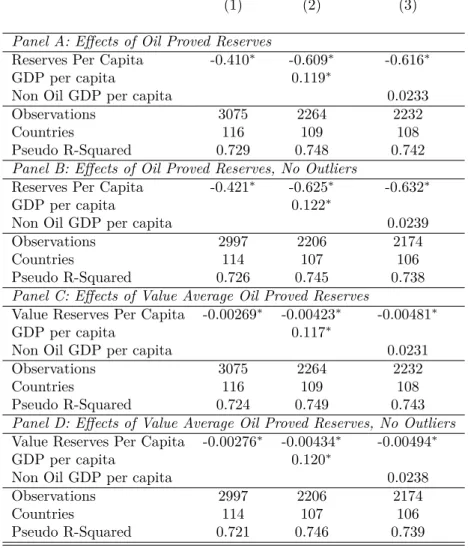
(13) 8. 0. ARE KWT. VEN FJI CPV DOM MNG ARG PER LKA THA BRA PHL CHL PNG KOR NIC HND PAN MYS PRY MDG MEX SLV NPL GTM SUR SEN PAK BGD KEN COM GMB ZMB NER BEN LSO MOZ GUY IDN MLI NAM ZWE GHA GNB NGA IRN LAO MRT SGP TZA VNM CHN EGY MWI CAF SLE MMR MAR UGA HTI JOR AGO DZA DJI ETH TUN SDN GIN CMR BFA KHM RWA CIV GNQ SYR BHR GAB OMN TGO BDI ERI TCD SWZ BTN CUB LBR YEM PRK. QATSAU. BRN. 10. 20 30 Oil Reserves per capita Fitted values. 40. 50. IRQ. LBN SOM BLZ BHS MDV BRB COG. 0. 0. LBN SOM BLZ BHS MDV BRB COG. MUS CRI JAM INDTTO ECU BOL ZAF URY COL BWA TUR SLB. Executive Constraints 2 4 6. 8 Executive Constraints 2 4 6. MUS CRI JAM IND TTO ECU BOL ZAF URY COL BWA TUR SLB VEN FJI CPV DOM MNG ARG PER LKA THA BRA PHL CHL PNG KOR NIC HND PAN MYS PRY MDG MEX SLV NPL GTM SUR SEN PAK BGD KEN COM GMB ZMB NER BEN LSO MOZ GUY IDN MLI NAM ZWE GHA GNB NGA LAO MRT SGP TZA VNM CHN EGY MWI IRN CAF SLE MMR MAR UGA HTI JOR AGO DZA DJI ETH TUN SDN GIN CMR BFA KHM RWA CIV OMN GAB GNQ SYR BHR TGO BDI ERI TCD SWZ BTN CUB LBR YEM PRK IRQLBY. LBY. QAT. BRN. 0. 5. Executive Constraints. 10 Oil Reserves per capita. Fitted values. Executive Constraints. 8. Figure 2: Executive Constraints versus Oil Proved Reserves per capita, No Outliers. 8. Figure 1: Executive Constraints versus Oil Proved Reserves per capita, Full Sample. 15. IND. TTO BOL COL. TUR. 0. BLZ BHS MDV. ZAR. 2. BRB. COG. 4 6 Oil and Gas Production Fitted values. MUS JAM CRI BOL ECU. VEN FJI CPV DOM MNG ARG PER LKA BRA PNG THA CHL KOR PHL NIC HND TWN PAN MYS PRY MDG MEX SLV NPL GTM PAK SUR SEN BGD KEN COM GMB ZMB NER BEN LSO MOZ GUY IDN MLI NAM ZWE GNB NGA LAO MRT SGP TZA VNM CHN EGY MWI GHA IRN CAF SLE MMR UGA MAR HTI JOR AGO DZA DJI ETH TUN SDN GIN CMR BFA KHM RWA CIV OMN GAB GNQ SYR BHR TGO BDI TCD ERI SWZ BTN CUB LBR YEM PRK LBY IRQ LBN SOM. 0. IND. ECU. Executive Constraints 2 4 6. Executive Constraints 2 4 6. ZAF URY BWA SLB. QAT. URY. CPV LKA PHL PNGNIC HND. MDG. VEN. FJI DOM THA PER. BRA CHL PAN MYS PRY SLV GTM SUR. NPL PAK BGD SEN KEN GMB COM ZMB NER BEN LSO MOZ IDN GUY MLI NAM GHA GNB TZA LAO VNM NGA MRT CHN ZWE EGY MWI IRN CAF SLE UGA MAR HTI JOR AGO DJI DZA ETH TUN SDN GIN CMR BFA KHM RWA CIV SYR GNQ BDI TCD ERI TGO SWZ BTN LBR YEM IRQ. ARG KOR MEX. SGP. GAB. OMN BHR. LBY LBN. BRN. 8. MNG. TTO. ZAF COL BWA TUR. SLB. ZAR. 0. CRI JAM MUS. 10. 5. Executive Constraints. COG. 6. Fitted values. Figure 3: Executive Constraints versus Oil Production per capita. MDVBLZ. 7 8 GDP per Capita. BRB. 9. Executive Constraints. Figure 4: Executive Constraints versus GDP per capita. endogenous than reserves, since it is easier to vary production than it is to vary reserves, which are highly inelastic and will only change if new discoveries are made. The slope is slightly negative, and Kuwait and The United Arab Emirates no longer appear as outliers. At first sight, it might seem as though the effect of oil on checks and balances is not very significant, and that these correlations cannot say much. However, once one takes into account the correlation with GDP per capita, which is positive with Executive Constraints and also positive with Oil reserves/production, as shown in figure 4, we might find a stronger effect of oil on executive constraints. The OLS regressions presented in Table 2 look to identify the correlation between our variables of interest, and to test the statistical significance of the sign of the slope shown in the figures above. We can see that the correlation between executive constraints and oil reserves is negative for all specifications, however when we consider. 11. BRN BHS. 10.

(14) the full sample it is only significant once we take into account GDP per capita. Once we drop the outliers, the correlation is negative and significant, and the coefficients grow considerably, as displayed in columns 3 and 4 of Panel A. The results for oil and gas production are similar, but they are only significative once we take into account the correlation with GDP per capita, as can be seen in columns 2 and 4 of Panel B. The coefficients are higher given the logarithmic scale used in the measurement of this variable. Although cross section OLS regressions of this kind do not establish causality, and are subject to omitted variable bias, these simple regressions are a first approach, and shed some light into the relationship between our variables of interest. If we can see a negative relationship between oil reserves/production and executive constraints in cross section OLS regressions, this may indicate that there is a possible causal effect which could be measured more accurately using panel data and more elaborate statistical methods. It seems that oil, whether we consider oil reserves or oil production, has a negative correlation with executive constraints, this is countries with larger oil reserves have lower checks and balances, especially once we take into account the income effect of GDP per capita.. Table 2: Cross Section OLS: Simple Correlations (1) (2) Full Full Sample Sample Panel A: Correlation with Oil Proved Reserves Oil Reserves per capita -0.0367 -0.0540+ GDP per capita 0.240 Observations 116 110 R-Squared 0.0133 0.0354 Panel B: Correlation with Oil and Gas Production Oil/Gas Production per capita -0.0778 -0.160∗ GDP per capita 0.367∗ Observations 116 110 R-Squared 0.0147 0.0586 +. 2.2. p < 0.10,. ∗. (3) Excluding Outliers. (4) Excluding Outliers. -0.312∗. -0.646∗ 0.382∗ 107 0.113. 113 0.0533 -0.0653 113 0.00899. -0.138∗ 0.399∗ 107 0.0592. p < 0.05. Oil Prices and the Effects of Price Shocks. A main implication of our model is that countries should choose lower equilibrium checks and balances when the value of their oil reserves is larger. We exploit the time variation of oil prices to account for this variation in the value of their reserves, thus, we should expect positive price shocks to lead to lowering equilibrium checks and balances in oil producing countries, while negative price shocks should lead to raising equilibrium checks and balances. This section provides some visual evidence which motivates our use of the variable “Value of Average Reserves per Capita”, which exploits the time variation of oil prices. 12.

(15) 100 80 40 20. 20. 40. Oil Price 60. Price of Oil 60. 80. 100. which is exogenous for most countries except for Saudi Arabia. In this sense, we are adding another dimension to the effects of natural resources, allowing for the value of the resources to change political incentives, so that oil prices can have an effect on political outcomes. This is interesting because it has not been studied in detail in past literature, and could provide a more exogenous way to identify effects of natural resources. Figures 5 and 6 show the evolution of the price of oil through time, Figure 5 shows positive price shocks, while figure 6 shows the negative price shocks identified. We have defined periods of “shocks” as those where there is a distinct change in the evolution of the price, and where the yearly change was more than 10% per year for a prologued period (2 years or more). For instance, in the first positive price shock between 1988 and 1990, the price of oil rose by about US$13, which meant a rise of 44%, around 20% per year. The second positive price shock was identified between 1998 and 2000. The price of oil rose by US$20, which meant a rise of 110%. This means the price more than doubled during this period. The last positive price shock identified is a longer time period (4 years) from 2002-2006. During this period, oil prices rose steadily at around 30% per year, which meant an overall rise of 132% in the four year period.. 1980. 1985. 1990. 1995. 2000. 2005. 1980. Year + Price Shock + Price Shock. 1985. 1990. 1995. 2000. Year + Price Shock Price of Oil. - Price Shock - Price Shock. Figure 5: Positive Shocks. - Price Shock Price of Oil. Figure 6: Negative Price Shocks. Figure 6 presents the negative shocks. The first negative price shock is identified between 1980 and 1983. During this time frame, the price of oil fell by US$34.5, a drop in 34% of its value. The second period of shock exhibits a fall of US$30 during the full period, which accounts for a fall of 52% of the value of the price at the beginning of the shock. Finally, we see a negative price shock between 1996 and 1998, during which the price of oil fell by US$13, which meant a fall of around 40% of the initial value. Figures 7 and 8 show the evolution of average executive constraints through time for oil producers (dashed lines), non oil producers (dotted line) and all countries in our sample. We have marked the years corresponding to positive price shocks on Figure 7 and negative price shocks on Figure 8. According to our hypothesis, we should observe raising checks and balances in oil producing countries during years marked as negative shocks, and decreasing checks and balances in oil producing countries during years marked as positive shock years.. 13. 2005.

(16) 4.5 2. Executive Constraints 2.5 3 3.5 4. 4.5 Executive Constraints 2.5 3 3.5 4 2. 1980. 1985. 1990. 1995. 2000. 2005. 1980. 1985. 1990. Year + Price Shock 1 + Price Shock 3 Oil Producing. 1995. 2000. Year + Price Shock 2 All Non Oil Producing. - Price Shock 1 - Price Shock 3 Oil Producing. Figure 7: Executive Constraints: Positive Price Shock. - Price Shock 2 All Non Oil Producing. Figure 8: Executive Constraints: Negative Price Shock. During the first positive price shock, average executive constraints fell from 2.75 to 2.55 in oil producing countries, which represents a fall of around 7.3%. In non oil producing countries, the change was positive and represented a 14% raise. Executive constraints remained virtually unchanged for oil producing countries during the second positive price shock, however during the third positive price shock they fell by 0.3, which meant an 8.8% difference, while non oil producing countries exhibit a raise in their average constraints of 10%. A similar pattern can be observed for negative price shocks. During the first price fall, average constraints rose by 24%, and oil producing countries showed higher average constraints on the executive than non oil producing countries for the only time frame in our sample. The second significant fall in prices shows a small rise in average constraints for oil producing countries of just 0.05, or 1.9%, and constraints do not seem to move differently in oil producing versus non oil producing countries. The third oil price fall however, came accompanied by a rise of 19% in average constraints for oil producing countries, while non oil producing countries show a fall of almost 4%. It seems, from these graphs, that the effects of oil price shocks are more evident when the shock is negative, however, one has to take into account other “time effects”, for example, the fact that executive constraints show a tendency to be increasing over time, both for oil producing and non oil producing countries. This could be a product of income growth, or the gradual acceptance of more widespread use of democratic principles and processes.. 2.3 Probability of Dismantling and Raising Checks and Balances Another dimension which is interesting to analyze is if countries with larger oil reserves/production are more likely to dismantle or raise their checks and balances. Instead of analyzing (continuous) equilibrium checks and balances, we will examine the more discontinuous measures of raising and dismantling checks and balances. The fact. 14. 2005.

(17) that oil producing countries seem to dismantle checks and balances more when there are positive price shocks and raise checks and balances more when there are negative price shocks is evidence of a possible effect of oil prices on executive constraints. In this sense, this section provides us with some stylized facts which are interesting and motivate our more elaborate statistical identification presented in Section 5, where we establish causal effects of oil on checks and balances. We define dismantling checks and balances as passing from a higher value of executive constraints to a lower one, and raising checks and balances as passing from a lower value of executive constraints to a higher one. We should expect the number of times an oil producing country dismantles checks and balances to be higher during positive price shock years than during non positive price shock years. Conversely, we should expect the number of times an oil producing country raises checks and balances to be higher during negative price shock years than during non negative price shock years.. Table 3: Changes in Checks and Balances and Oil Price Shocks. Oil Producing. Non Oil Producing. ∆+ Prices ∆− Prices ∆0 Prices Difference t-Test p-value ∆+ Prices ∆− Prices ∆0 Prices Difference t-Test p-value. ∆ Checks and Balances Dismantle Raise 0.0346 0.0545 0.0178 0.0293 0.0168* 0.0252+ 0.0293 0.0591 0.0394 0.0502 0.0273 0.0600 0.0122 -0.0097 0.1314 0.3494. + p < 0.10, * p < 0.05. Table 3 shows the result of comparing the number of dismantles/rises during price shock years divided by the number of positive price shock years, versus the number of dismantles/rises during non positive price shock years divided by non price shock years for oil producing and non oil producing countries. It is clear that oil producing countries dismantled more during positive price shock years, and the difference is significative at a 5% level. For the raising of checks and balances we observe a similar phenomenon, however, the p-value for the t test is higher, and equal to 0.591, which means that this difference can only be accepted at a 10% confidence level. For non oil producing countries, we can see that the number of dismantles/rises during price shock years does not significantly differ from the number of dismantles/rises during non price shock years. This is, again, attests to the fact that the value of oil reserves in a country affect the incentives to dismantle/raise checks and balances, and is evidence to support our hypothesis that oil producing countries will be more likely to dismantle checks and balances when there are positive oil price shocks. These simple exercises shed some light on the correlation between executive con-. 15.

(18) straints and oil reserves/production in developing countries, and of the possible effects that oil, and oil prices, may have on this institutional measure. The next section develops a model which explicits the mechanisms through which the presence of oil could alter institutional decisions such as equilibrium checks and balances and the decision to dismantle or raise executive constraints. The sections following this will present a more thorough econometric estimation of the effects.. 3. A Model for Endogenous Checks and Balances. The model we develop is based on the work of Acemoglu, Robinson and Torvik (2013). We extend the model to include a measure of resource abundance. The model considers a static economy with a continuum of agents which is normalized to 1. A portion 1 − δ > 1/2 are poor with pre tax income y p > 0. A portion δ are rich, with income y r > y p . The utility of the representative agent from group i ∈ p, r is U j = cj Average income per capita is thus ȳ = (1 − δ)y p + δy r We also define θ ∈ [0, 1] as the measure of income inequality, as it represents the share of the total income which goes to the rich i.e, θ ȳ δ (1 − θ) yp = ȳ 1−δ yr =. 3.1. Policies and the Constitution. The government is formed by a legislator and a president, which can belong to the poor income group or the rich income group, so a politician can be from income group i ∈ {p, r} and hold office j ∈ {L, P }, standing for Legislator or President. The president and legislator must determine tax rates, τ ∈ [0, τ̄ ], which will determine the governments income. They must also determine the amount of redistribution through transfers to the rich and poor, {τ, T r , T p } respectively, and they must set the level of rents for politicians: {RP , RL }, which represent rents for the president and legislator respectively. In the original model, the government just received income from taxes, however we have extended the model to include a natural resource measure, which captures the fact that most natural resources are state owned, and that the rents from the exploitation of these resources goes straight to the hands of the government. This is relevant because it modifies the government’s budget constraint, thus altering the behaviour that government agents will exhibit. The members of the government must now determine the full vector of policies, subject to its budget constraint: (1 − δ)T p + δT r + RL + RP ≤ τ ȳ + ηN. 16. (1).

(19) The ηN component of the equation was not present in the original model, and is crucial to understanding the effects of oil on checks and balances. It represents the amount of rents the government receives from its natural resource market. η represents the proportion of the resource rents which the government can extract and N represents the value of the resource production in the economy (size of the oil industry). We assume that the proportion 1 − η goes to international oil companies and thus does not appear in the rest of the model, this assumption is realistic given that most of the ownership of oil fields is either in the hands of NOCs or of large international oil firms. According to Ross (2012), resource rents are different from tax revenue, and more detrimental, because of their large scale, unusual source, lack of stability and their secrecy. Oil revenues have an exceptionally inelastic supply (it is very hard and investment intensive to vary production), and are usually the result of large scale projects. This means that oil revenues appear as a “flood” of new funds for the government, and thus present important variations to the government budget constraint once they appear. The size of oil rents varies strongly with oil prices, which can be volatile, thus generating a source of uncertainty into future financing for the government. This usually results in governments spending oil revenues in a different way than how they would spend their tax revenues, which they can predict with more accuracy. Price volatility in the short run is mainly a result of the nature of the source described above: demand and supply of oil are very price inelastic, so neither suppliers or consumers can adjust to changes in prices in a swift manner. This results in shocks generating large price changes. In fact, since 1970, the price of oil has changed by an average of 26.5 percent a year10 . The secrecy of oil revenues means that these rents are “unusually easy for governments to conceal”11 . In fact, a study on the subject found that “secrecy in the extractive industries is so commonplace that until recently, neither states nor companies have felt compelled to develop sophisticated arguments to defend it.”12 . For our analysis we will not consider the “secrecy” dimension of oil revenues, however this could be captured by the η component, which could capture how much of the rents are known to public, and thus available information for them to make their decisions when voting on checks and balances. Furthermore, oil revenues are not subject to the same amount of accountability than tax revenue is. Tax payers expect the government to use their funds effectively, and to receive something in return for their taxes. The very nature of oil revenues (size, secrecy, volatility) makes it harder for the population to hold the government accountable for the way in which they spend this money. Many governments in weakly institutionalized countries prefer to charge less taxes and spend more of their oil revenues in a clientelistic way, thus becoming less accountable and more popular. The way in which policies are determined will vary depending on the presence of checks and balances in the constitution. If the constitution includes checks and balances, denoted by γ = 1, the president decides the taxes and the transfers {τ, T r , T p }, and the legislator can then choose the rents for each political institution {RP , RL }. If 10. Ross (2012) based on data from BP Statistical Review of World Energy, 2010 Ross (2012). 12 Rosenblum and Maples 2009,12. 11. 17.

(20) the constitution does not involve checks and balances, γ = 0, the president decides the full vector of policies: {τ, T r , T p , RP , RL }, and the legislator has no significant power. Politicians derive utility from their own rents and from the rents of their income group. This is a reduced form way of capturing political ideology and the fact that politicians will usually have family or social ties with people in the same income group as them. The utility of the politicians is quasilinear in U i , so the utility of a politician from income group i ∈ {p, r} holding office j ∈ {L, P } is V j,i = αν(Rj + bj ) + (1 − α)U i. (2). Where α denotes the relative preference between his own rents and those of his income group (also could represent strength of ideology), ν is a strictly concave, strictly increasing and continuously differentiable function which represents the utility of the politician derived from rents and bribes. This function also satisfies the Inada type conditions, and we normalize ν(0) = 0. Note the presence of bj , which denotes the bribes which can be made by an organized elite to politicians, in order to sway them towards better policies for them. The president and the legislator are democratically elected by majority vote. Without loss of generality, we assume that for both the presidential and the legislative elections, there is one member of the poor group and one member of the rich group, randomly selected from each income group. Since 1 − δ ≥ 12 , the poor have an electoral advantage, and so the president and the legislator will always be from the poor group. The rich, however, can come together and bribe the politicians to their advantage. The elite will be able to solve their collective action problem with a probability q ∈ [0, 1]. κ = 1 denotes that the rich have solved their collective action problem and can bribe politicians, while κ = 0 denotes the contrary. If κ = 1 then the rich can pay a bribe B = bL + bP , which is paid equally by each agent in the group, so that each agent pays B/δ. The utility of a representative agent of each income group is then given by U p = (1 − τ )y p + T p U r = (1 − τ )y r + T r −. bL + bP δ. .. 3.2. Timing of Events. The timing of events is: 1. Referendum on whether the constitution includes checks and balances (γ = 0 or γ = 1). Absolute majority wins. 2. Elections for president and legislator. Absolute majority wins. 3. All uncertainty is revealed (whether the elite will solve their collective action problem or not). 4. If collective action problem is solved, the elite make bribe offers to politicians. 5. If the constitution does not include checks and balances, the president decides {τ, T r , T p , RP , RL }. If the constitution includes checks and balances, then the. 18.

(21) president first decides on {τ, T r , T p }. After this, the legislator can choose the rents for the politicians, {RP , RL }. 6. Policies are implemented, bribes are paid and all payoffs are realized. We will focus on subgame perfect equilibria in undominated strategies13 , as a way of ruling out unreasonable equilibriums which may arise given the multiple rounds of voting which take place in this game. To identify the equilibrium, we use backward induction and finally arrive at the SPE . Without loss of generality, the analysis will be limited to the election of members of their own group by the poor, given that it is always optimal for them to vote in this way, even including the possibility of bribes. Given the electoral advantage of the poor, all politicians will be from the poor income group.. 3.3. Equilibrium Without Checks and Balances. Let us suppose that the referendum led to a constitution without checks and balances, this is γ = 0. In this case, the president can choose all policies, ignoring the legislator. Let’s first consider the case when κ = 0, so the rich could not solve their collective action problem and thus will not be able to bribe any politicians. The president maximizes: V P,p [γ = 0, κ = 0] = max{τ,T p ,T r ,RL ,RP } αν(Rp )+ (1 − α)((1 − τ )y p + T p ) subject to the government constraint (1), T p , T r , RL , RP ≥ 0 and τ ≤ τ̄ . Given that ν is strictly concave, this problem has a unique solution. Incomes will be taxed at the highest rate, τ̄ , and all proceeds will be spent on transfers to the poor and rents for the president, R∗ such that αν 0 (R∗ ) =. 1−α 1−δ. (3). The transfers to the poor will thus be T p = (τ̄ ȳ + ηN − R∗ )/(1 − δ), and the utility for a poor agent in this scenario will then be U p [γ = 0, κ = 0] =. (1 − θ + τ̄ θ)ȳ + ηN − R∗ . 1−δ. 13. (4). In game theory, a subgame perfect equilibrium (or subgame perfect Nash equilibrium) is a refinement of a Nash equilibrium used in dynamic games. A strategy profile is a subgame perfect equilibrium if it represents a Nash equilibrium of every subgame of the original game. Informally, this means that if (1) the players played any smaller game that consisted of only one part of the larger game and (2) their behavior represents a Nash equilibrium of that smaller game, then their behavior is a subgame perfect equilibrium of the larger game. Every finite extensive game has a subgame perfect equilibrium. An Introduction to Game Theory, Osborne, M.J., Oxford University Press, USA, 2004. Acemoglu, Egorov and Sonin (2009) propose sequentially eliminating weakly dominated strategies, or the slightly stronger concept of Markov Trembling Hand Perfect Equilibrium proposed by Selten (1975). All equilibriums analyzed here are in fact Markov Trembling Hand Perfect Equilibria.. 19.

(22) Now lets suppose κ = 1, so that bribe offers are made. The bribe offers must satisfy V P,p (b̂P , τ̂ , Tˆp , Tˆr , RˆP ) ≥ V P,p [γ = 0, κ = 0] ≡ αν(R∗ ) + (1 − α). (1 − θ + τ̄ θ)ȳ + ηN − R∗ 1−δ. (5). Thus, imposing bL = 0, the problem of the rich lobby is U r = max(b̂P ,τ̂ ,Tˆp ,Tˆr ,RˆP ) (1 − τ̂ )y r + T̂ r −. b̂P δ. subject to (1), (5) and to τ̂ ≤ τ̄ . If this gives the rich less than U r [γ = 0, κ = 0] then they will prefer to not give bribes. Without checks and balances, the rich will never offer bribes.14 In this case, the president will make all policy decisions, and the utility of the poor will be the same whether the rich solve their collective action problem or not, i.e. U p [γ = 0, κ = 0] = U p [γ = 0, κ = 1] = U p [γ = 0]. The intuition behind this result is interesting. The lack of constraints on the president allows him to maximize his utility and obtain his bliss point, which in turn makes him very expensive to bribe. This means that by having no checks and balances, the poor are “protected” from the adverse effects of elite capture on their utilities. This is the mechanism which could lead voters to rationally dismantle checks and balances when there is a threat of elite capture. They chose to give the president (who comes from their own income group) more power, allowing him to extract more rents, in order to avoid capture by the elite which would lead to unfavourable policies for the poor. Proposition 1 When the constitution has no checks and balances, γ = 0, then regardless of κ, the equilibrium will be τ = τ̄ , RP = R∗ , RL = 0, bP = bL = T r = 0, and T p = (τ̄ ȳ + ηN − R∗ )/(1 − δ). The utility of the poor is given by (4). Natural resources raise the value of the transfers to the poor. This is due to the fact that the president has the liberty to obtain his bliss point with income from taxes, and thus redistributes the remainder of the government’s income to the poor. No checks and balances gives the president more power to extract rents for himself, making him too expensive to bribe by the rich, and thus protecting the poor from the possible unfavourable policies (no redistribution) which could be applied if κ = 1 and the rich could bribe the president. This means that natural resources raise the funds available for redistribution to the poor, regardless of the presidents “corruption”, and no checks and balances ensure that this redistribution takes place. In this sense, natural resources make the equilibrium with no checks and balances more attractive for the poor, by raising their income after government transfers. The poor are willing to allow some “corruption” from the president as long as he redistributes to them, which is only possible if he is not captured by the elite. It is interesting to note that when there are no checks and balances there is no threat of elite capture, so that under any scenario of κ, more natural resources raise the utility of the 14. Proof of this is in Appendix A.. 20.

(23) poor. Given the nature of this income, the natural resource component changes the incentives for the poor in a significative way, countries with large reserves will display very large potential transfers for the poor in comparison to the cases where there is no income from natural resources.. 3.4. Equilibrium Under Checks and Balances. Let us now analyze the case when the referendum has led to a constitution with checks and balances, so that γ = 1. Let’s consider first when κ = 0, so no bribes will be made. In this case, the legislator solves: V L,p [γ = 1, κ = 0] = max{RL ,RP } αν(RL ) + (1 − α)((1 − τ )y p + T p ) subject to (1), and to {τ, T p , T r } elected by the president. The solution to this maximization problem is RP = 0 and RL = τ ȳ − (1 − δ)T p − δT r . Given this, the president solves the following problem in the prior subgame V P,p [γ = 1, κ = 0] ≡ max{τ,T p ,T r } αν(RP ) + (1 − α)((1 − τ )y p + T p ) subject to (1), τ ≤ τ̄ , and to the best response of the legislator (RP = 0). Given that RP = 0, the president will maximize the utility of the poor, and leave the legislator with no rents. The utility of the poor will be maximized at U p [γ = 1, κ = 0] =. (1 − θ + τ̄ θ)ȳ + ηN > U p [γ = 0] 1−δ. (6). The intuition behind this result is that with checks and balances, the legislator has the power to take rents away from the president and towards himself. This leads the president to maximize the utility of the poor in the prior subgame, and leave no rents for politicians. The utility of the president is lower than before, since he cannot choose the level of rents that leaves him at his bliss point. V P,p [γ = 1, κ = 0] = (1 − α). (1 − θ + τ̄ θ)ȳ + ηN < V P,p [γ = 0, κ = .] 1−δ. More control over the president leads to higher redistribution and more well being for the poor, however, if the rich are able to solve their collective action problem, more checks and balances could become a double edged sword. This is because the president is worse off with checks and balances, and thus becomes cheaper to buy by the elite. Bribes by the rich elite could lead the president to lower redistribution and thus leave the poor worse off. If κ = 1 the elites will offer bribes {b̂L , R̂L , R̂L } and {b̂R .τ̂ , T̂ p , T̂ r } to the legislator and president, respectively. The bribes must satisfy the participation constraints in. 21.

(24) order to be accepted. We know bL = 0, and also RP = 0. Without loss of generality, we will focus on cases where T r = 0. So, the problem of the elite is max{b̂P ,T̂ p ,τ̂ } (1 − τ̂ )y r −. τ̂ ȳ + ηN − (1 − δ)T̂ p b̂P + δ δ. subject to. αν(b̂P ) + (1 − α)((1 − τ̂ )y p + T̂ p ) ≥ (1 − α)((1 − τ̄ )y p +. τ̄ ȳ + ηN ) 1−δ. Tˆp ≥ 0, τ̄ ≥ τ̂ The solution to this problem is represented in Proposition 215 : Proposition 2 When the constitution involves checks and balances, then: 1. When κ = 0 so there is no bribing, the equilibrium involves τ = τ̄ , RP = RL = T r = 0, T p = (τ̄ ȳ + ηN )/(1 − δ), and the utility of the poor is given by (6). 2. When κ = 1 so that there is an organized elite, there is an α∗ ∈ (0, 1) such that: (a) If α > α∗ , then τ = τ̄ , RP = RL = bL = T p = 0, bP > 0, T r > 0. (b) If α < α∗ , then τ < τ̄ , RP = RL = bL = 0, T p > 0,bP > 0,T r ≥ 0. The expected utilities are then given by: If α > α∗ , then the expected utility of the poor is given by (1 − θ + τ̄ θ)ȳ + (1 − q)ηN − qτ̄ȳ 1 −δ ∗ If α < α , then the expected utility of the poor is given by U p [γ = 1 ] =. (7). ∗. p. U [γ = 1 ] =. ) (1 − θ + τ̄ θ)ȳ + ηN − q νν(R 0 (R∗ ). 1 −δ. (8). We can see here that checks and balances are only effective in reducing politician rents and raising redistribution if the rich elite cannot solve their collective action problem. When the rich cannot bribe politicians, checks and balances act as a mechanism to keep politicians from abusing their power and becoming corrupt, so that no extraction is made on behalf of politicians and the poor are better off. However, if the rich are able to organize and bribe politicians, checks and balances have an adverse effect by making the politicians cheaper to bribe. This means that policies will no longer favour the poor, and the politicians and the rich will be better off, at the expense of the poor, reducing the utility of the poor voters. When α > α∗ , the extent to which natural resources raise the expected utility of the poor, given that there are checks and balances, depends on q, the probability 15. Proof of this proposition can be found in Appendix B. 22.

(25) that the elite will solve their collective action problem, while the positive effect on the expected utility given there are no checks and balances does not. This means that higher values of ηN involve a higher relative loss for the poor if the elite manage to bribe the president. This leads to an amplification of the effect proposed by Acemoglu et al (2013), where higher natural resource rents will lead to greater difference in the utility of the poor depending on whether or not the elite could bribe the president. The fact that there is a limit on how many taxes the government can charge, and the considerable size and inelastic nature of N makes the effect of natural resources very significant. It means that the poor have great incentives to avoid elite capture, because their potential gains from doing so are very large. In this sense, when there is a high probability of elite capture, as was the case in countries like Venezuela, Ecuador and Bolivia, it becomes very attractive for the poor majority to vote for the dismantling of checks and balances when oil revenues are substantial. By allowing some “corruption” on behalf of the president, they are insuring large transfers for themselves, a small price to pay when one considers the alternative outcome.. 3.5. Elections. It will always be the dominant strategy for a person of any income group to vote for the politician of such income group, regardless of whether it is a presidential election or a legislative election. Without checks and balances, a rich candidate would charge the same taxes τ̂ but would not redistribute to the poor, so the poor will strictly prefer a candidate from the poor income group. Because there are no checks and balances, the legislator has no power so the poor are indifferent between a poor or a rich legislator. When there are checks and balances, if there is no bribing, the president from the poor group will simply maximize the utility of the poor, thus it is optimal for the poor to vote for a member of their own group. When the rich can offer bribes, the president from the rich group will not offer any redistribution to the poor, while the president from the poor group will offer some, so it is strictly better for a poor agent to vote for a president from his same group. Thus, it is a weakly dominant strategy for the poor to vote for a member of their own group in a presidential election. We will assume that the legislator will also be from the poor group, although this has no real impact on the final results because he simply distributes rents between him and the president.. 3.6. Referendum and Equilibrium Checks and Balances. In this stage of the game voters must decide whether or not they want a constitution with checks and balances. This depends on whether the expected utility, before knowing if the rich can solve their collective action problem or not, is greater with checks and balances or without them.. 23.

(26) Proposition 3 1. Suppose that α > α∗ . Then the constitution will involve no checks and balances, i.e., γ = 0, if R∗ (9) q> τ̄ȳ + ηN and it will involve checks and balances if the converse holds. 2. Suppose that α < α∗ . Then the constitution will involve no checks and balances, γ = 0, if ν 0 (R∗)R∗ q> , (10) ν(R∗ ) and it will involve checks and balances if the converse holds. This is the main result of our extension. Countries with larger oil industries, and countries which can extract a larger share of the rents produced by oil industries, will be more likely to have lower equilibrium checks and balances. This can be seen in equation (9), where larger ηN implies that the constitution will not include checks and balances for a larger set of q. This implies that the probability of a country choosing low checks and balances (or no checks and balances in this case) grows when oil revenues are larger. Equation 9 is capturing the trade-off between higher rents for the poor with checks and balances if there is no elite capture and lower rents for the poor with checks and balances if there is elite capture. The difference in the size of these potential rents depends, of course, on the tax revenue τ̄ ȳ, and on the size of the natural resource component, ηN . The larger the rents from natural resources are, the more valuable it is for the poor to avoid elite capture, and thus the more valuable it is for them to prevent the possibility of the elite capturing the executive power. This means that when they have to vote on the constitution, without knowledge of the ex-post result, they will be more likely to vote in favour of dismantling checks and balances when natural resource rents are higher, because the potential benefits of avoiding elite capture are very high. In other words, their expected returns without checks and balances become very high with large natural resource rents. This fully captures one of the possible channels through which natural resources may be affecting endogenous equilibrium checks and balances. The extension becomes specially interesting once one compares the size of τ̄ ȳ with ηN , where the latter can be so big that it generates an undeniable effect on the equilibrium. The results of Acemoglu, Robinson and Torvik are the same as the results presented in Propositions 1, 2 and 3, but assuming ηN = 0. We can see that equation 9 is modified by the extension but equation (10) remains unchanged. Our extension, which seems very simple, opens up a whole new area of predictions, and makes the model applicable to a different literature than the one it was initially intended. It captures a strong effect of natural resources on institutions, which up to now had not been identified clearly by a straightforward model.. 24.

(27) 3.7 Extension: Relaxing the Quasilinearity of the Utility Function In this section we will relax the quasilinearity of the utility function, and test the implications of using V j,i = (Rj + bj + r)β (U i )1−β , as the utility function of the politicians. Throughout, we suppose that r > 0 represents ego rents of becoming an elected politician, and for simplicity of the comparison of both models, we assume that r → 0, so that these rents eventually vanish. In this case we have that: τ̄ ȳ+ηN Proposition 4 Let β H ≡ (1−θ+τ̄ θ)ȳ+ηN and suppose that r → 0 . Then: H 1. When β > β the constitution will always involve checks and balances. 2. When β < β H then the constitution will involve no checks and balances if. q>. β[(1 − θ + τ̄ θ)ȳ + ηN ] τ̄ȳ + ηN. (11). Proof: Let us first consider the case where the constitution involves no checks and balances, i.e. γ = 0. In the case where κ = 0, so the rich lobby are not able to solve their collective action problem, the president will solve the following problem in the policymaking subgame: V P,p [γ = 0, κ = 0] = max{τ,T p ,T r ,RL ,RP } (RP + r)β ((1 − τ )y p + T p )1−β. (12). subject to the government budget constraint. This problem has a unique solution where incomes are taxed at a maximum rate, with all proceeds spent on rents to the president and transfers to the poor. Next, let’s suppose that κ = 1, so the rich lobby can offer bribes. Given that the constitution involves no checks and balances, it will never be benefitial for the lobby to offer bribes, so b̂P = 0. Proposition 4.a Suppose γ = 0. Let r → 0, and τ̄ (13) 1 − θ + τ̄ θ Then the equilibrium policy always has τ = τ̄ . Moreover: 1. if β > β H , then T p = 0. The utility of poor agents in this case is U p [γ = 0] = (1 − θ)(1 − τ̄ )ȳ/(1 − δ); 2. if β < β H , then transfers are given by βH =. T p = (τ̄ − β(1 − θ + τ̄ θ)). 25. ȳ (1 − β) + ηN 1−δ 1−δ. (14).