The economic effects of interregional trading of renewable energy certificates in the WECC

Texto completo

(1)PONTIFICIA UNIVERSIDAD CATOLICA DE CHILE ESCUELA DE INGENIERIA. THE ECONOMIC EFFECTS OF INTERREGIONAL TRADING OF RENEWABLE ENERGY CERTIFICATES IN THE WECC. ANDRES PABLO PEREZ. Thesis submitted to the Office of Research and Graduate Studies in partial fulfillment of the requirements for the Degree of Master of Science in Engineering.. Advisor: ENZO ENRIQUE SAUMA. Santiago de Chile, August, 2014  2014, ANDRES PABLO PEREZ.

(2)

(3) To my parents, who have inspired, motivated and supported me at all times. Both have taught me to be passionate about everything I do.. ii.

(4) ACKNOWLEDGEMENTS. First of all, I would like to thank my advisor, Prof. Enzo Sauma, for his continuous support during my studies in the M.S. Program at PUC. During the past few years I have enjoyed not only his expert technical guidance, but also his mentoring and advice. I have to credit his motivation and advice for leading me to reach high quality results in my research as well as in completing my program successfully. I would also like to thank Prof. Ricardo Paredes and Prof. Vladimir Marianov for agreeing to be part of my Examination Committee and for proposing challenging questions about my research. I am deeply grateful to Prof. Benjamin Hobbs, who received me warmly at The Johns Hopkins University. His passionate interest in the electricity markets motivated me even more in my thesis work. Also, my thanks to Dr. Francisco Muñoz, from whom I learned a lot about models during my internship at Johns Hopkins, and who also motivated me to participate in the world of research. I want to thank him for agreeing to be part of the Examination Committee. And in general I want to extend my appreciation to the professors from whom I learned a great deal during my time at PUC. In particular I am indebted to Prof. Fernando Arenas, who inspired me with his passion for Math. I would also like to thank Prof. Nicolás Majluf for enriching my views of the engineering profession. And on a personal level, I greatly appreciate the support of my family. I dedicate this thesis to my dear parents, Claudio and Patricia, who have guided my life. Both have supported me in every decision I have made and have taught me to be passionate about everything I do. They have always motivated me to make the most of my capacities. And I want to thank my brothers and sisters: Claudio, Patricia, Carolina, and Javier for being my joke partners when we were young (and even not so young). I would like to thank my school friends, my lifelong friends. To my girlfriend, Josefina, I thank you for your love, support, dedication, patience, and company during iii.

(5) the last three years. Your sense of humor, advice, and affection have really made a difference in my life. And I am thankful for all the great moments and adventures we have shared with the good friends I met in College. Some of these friends are Jaime, Antonio, Cristóbal, Josefa, Leslie, Felipe, Nicolás, Ignacio, and Sebastián. I am grateful to the Energy Group, with whom I have shared my academic life this past year. Finally, I thank the Centro de Alumnos de Ingenieria 2014 (CAi) who have supported me in many new initiatives and projects for graduate students.. iv.

(6) TABLE OF CONTENTS. ACKNOWLEDGEMENTS ......................................................................................... ii LIST OF TABLES ..................................................................................................... vii LIST OF FIGURES .................................................................................................. viii ABSTRACT ............................................................................................................... iix RESUMEN................................................................................................................... x 1.. INTRODUCTION .............................................................................................. 1 1.1 Renewable Portfolio Standards and Renewable Energy Certificates ........ 1 1.2 Transmission Expansion Planning ............................................................. 3 1.3 Motivation .................................................................................................. 4 1.4 Objective and Hypothesis .......................................................................... 5. 2.. SIMPLIFIED ANALYSIS OF TRADING IN A TWO-REGION EXAMPLE . 6. 3.. MODEL FORMULATION ................................................................................ 8. 4.. IMPLEMENTATION OF THE MODEL FOR THE WECC SYSTEM ......... 13 4.1. Description of the WECC 240 Bus Test Case ...................................... 13 4.2. Experiments Implemented in the WECC System Model ......................... 15. 5.. RESULTS AND DISCUSSION ....................................................................... 18 5.1. System Costs ............................................................................................ 18 5.2. Trading of REC ........................................................................................ 20 5.3. Generation Capacity Investments ............................................................ 22 5.4. Transmission Investments ........................................................................ 24 5.5. CO2 Emissions ......................................................................................... 26 5.6 Energy Prices ........................................................................................... 29. 6.. CONCLUSIONS .............................................................................................. 31 v.

(7) REFERENCES........................................................................................................... 34 APPENDICES ........................................................................................................... 38 APPENDIX A. COSTS OF THE SYSTEM .................................................... 39 APPENDIX B. RENEWABLE GENERATION ............................................. 41 APPENDIX C.EMISSIONS ............................................................................. 45. vi.

(8) LIST OF TABLES. 1. Renewable investment costs in each region.. .....................................................................6 2. RPS targets by state. .........................................................................................................14 A.1. Investments and operating costs (Billion dollar) versus trading allowed. Scenario 1. 39 A.2. Investments and operating costs (Billion dollar) versus trading allowed. Scenario 2. 39 A.3. Investments and operating costs (Billion dollar) versus trading allowed. Scenario 3. 40 A.4. Investments and operating costs (Billion dollar) versus trading allowed. Scenario 4. 40 B.1. Renewable generation (GWh-year) and required demand. Exporting and importing states in Scenario 1 for 25% of flexibility. ...........................................................................41 B.2. Renewable generation (GWh-year) and required demand. Exporting and importing states in Scenario 1 for 100% of flexibility. .........................................................................42 B.3. Renewable generation (GWh-year) and required demand. Exporting and importing states in Scenario 2 for 25% of flexibility. ...........................................................................43 B.4. Renewable generation (GWh-year) and required demand. Exporting and importing states in Scenario 3 for 25% of flexibility. ...........................................................................44 C.1. Emissions (Million metric tons of CO2) in California, New Mexico and Wyoming. Scenario 1. ............................................................................................................................45. vii.

(9) LIST OF FIGURES 1. Renewable goals as a fraction of the total electricity demand by year for states that belong to the WECC. .............................................................................................................2 2. (a) 1-Region scenario: No Geographic Restrictions. (b) 2-Regions scenario. (c) 3Regions scenario. (d) 4-Regions scenario. ...........................................................................17 3. Total Cost as a Function of Trading Flexibility.. .............................................................19 4. REC exports (white bars) and imports (gray bars) in the following cases: (a) 25% of REC trading is allowed in the 1-Region scenario, (b) 100% of REC trading is allowed in the 1-Region scenario, (c) 25% of REC trading is allowed in the 2-Regions scenario, and (d) 25% of REC trading is allowed in the 3-Regions scenario.. ..........................................21 5. Generation investments by technology in the 1-Region scenario, when (a) no REC trading is allowed, and when (b) 100% of REC trading flexibility is allowed.. ..................23 6. Aggregate transmission investment cost versus the percentage of trading allowed.. ......25 7. Transmission investment costs per state in the 1-Region scenario ..................................26 8. Aggregate WECC CO2 emissions as a function of the REC trading allowed. ................27 9. CO2 emissions per state in the 1-Region scenario. ..........................................................28 10. Average energy prices in the WECC and per state in the 1-Region scenario. ...............30 11. In-state REC generation by technology and state, in the 1-Region scenario. ................30. viii.

(10) ABSTRACT. In the U.S., states set their own Renewable Portfolio Standards (RPSs) for renewable electricity production, with little coordination. Each state imposes restrictions on the amounts and locations of qualifying renewable generation. I quantify the economic benefits of allowing increased trade of Renewable Energy Certificates (RECs) among the states belonging to the Western Electricity Coordinating Council (WECC) of the USA in order to meet state RPSs. Although more trade would be expected to have economic benefits, the magnitude of these benefits relative to the cost of additional transmission infrastructure is less certain. It is also unclear whether such trade would further pursue environmental objectives, namely greenhouse gas emissions reductions. I use a power transmission expansion planning model, formulated as a mixed integer program, to minimize the annualized investment and operations costs of the WECC system for year 2022. The model uses a 240 bus representation of the WECC network. I examine how total cost changes as I increase REC trading flexibility, as represented by both four distinct definitions of trading regions and different amounts of trading allowed. I also analyze impacts upon CO2 emissions and energy prices. The results show that if I increase the amount of RECs traded among states, the total cost decreases. Interestingly, the cost reduction is significantly large even for a relatively small level of trade. In particular, the total cost decreases by 10% when I allow 25% of RECs at state level being imported from any other state belonging to the WECC. When allowing even more trade, the total cost continues decreasing, but at a lower rate. As well, increasing REC trading flexibility does not seem to have a significant impact on CO2 emissions and/or energy prices (the WECC energy average price tends to slightly decrease). Keywords: Renewable Portfolio Standards, Renewable Energy Credits, transmission planning, WECC. ix.

(11) RESUMEN. En EE. UU., usualmente los Estados fijan Sistemas de Cuotas (RPS) para la producción de energía renovable con baja coordinación interestatal. Cada Estado impone restricciones en los montos y en la localización de los generadores que califican para cumplir las metas RPS. El principal objetivo de esta tesis es cuantificar los impactos económicos de transar Certificados de Energía Renovable (RECs) entre los estados pertenecientes a la Interconexión Oeste de la Red Eléctrica de Estados Unidos (WECC). Si bien, el intercambio de RECs debería traer beneficios económicos no se conoce la magnitud de tales beneficios ni los efectos en las emisiones del sistema. En este trabajo se utiliza un modelo de planificación de expansión de la transmisión, formulado como un programa entero mixto, que minimiza las inversiones anualizadas y los costos de operación del sistema para el año 2022. El modelo es aplicado en una representación de 240 nodos del WECC. Se estudian los costos totales del sistema a medida que se aumenta la flexibilidad, representada por límites en las restricciones geográficas y en los montos permitidos de transacción de RECs. Además se analizan los impactos en las emisiones de CO2 y en los precios de la energía. Los resultados muestran que al aumentar el intercambio de RECs, los costos totales del sistema disminuyen. Es interesante notar que la reducción de costos es significativamente grande incluso al imponerse un pequeño porcentaje de flexibilidad. En particular, los costos decrecen en un 10% cuando los Estados pueden importar un 25% de importación de RECs. Al permitir mayores grados de flexibilidad los costos continúan disminuyendo, pero a una tasa más baja. También al aumentar la flexibilidad parece no haber impactos significantes en las emisiones de CO2 ni en los precios de la energía (precio de energía promedio del WECC tiende decrecer ligeramente). Palabras Claves: Sistemas de Cuotas, Certificados de Energía Renovable, planificación de la transmisión, WECC. x.

(12) 1. 1. INTRODUCTION 1.1 Renewable Portfolio Standards and Renewable Energy Certificates. Climate change policies have been an important driver to encourage investments in power generation from renewable resources (Kung, 2012). Even when global pollutant emission policies – such as carbon taxes or cap-and-trade programs – do not specify renewable targets, they indirectly incentivize generation from renewable resources by making some conventional technologies less competitive (Fischer and Newell, 2008). In addition, some regulatory policies directly promote generation from renewables, such as Renewable Portfolio Standards (RPSs), Feed-in Tariffs (FITs), and Renewable Auction Mechanisms (RAMs) (Sauma, 2012a). Since the 1990’s, the RPS has proliferated as the most popular renewable policy implemented at the state level in the US (Wiser et al., 2007). To date, 37 states have defined renewable targets, but only 30 of them enforce their goals through noncompliance penalties (US DSIRE, 2013). Many arguments have been provided in order to justify RPS policies. Some states, such as Arizona, California, and Colorado, emphasize the competitiveness and the environmental benefits: “…competitive and friendly renewable electricity technologies”, “…ameliorate air quality problems throughout the state…”, “…to improve the natural environment of the state”. Other states, such as Montana and Washington, include other perspectives: “…fuel diversity, economic, and environmental benefits…”, “…stabilize electricity prices, provide economic benefits, create high quality jobs, and protect clean air…” (Holt and Wiser, 2007). The RPS design requires energy providers within a state to supply a fraction of their energy from renewable resources. Fig. 1 shows the evolution of renewable goals in the states belonging to the Western Electricity Coordinating Council (WECC) of the USA. These goals have different enforced timing structures. For instance, Arizona has set a specific goal every year while California has set only three different specific goals..

(13) 2. Fig.1. Renewable goals as a fraction of the total electricity demand by year for states that belong to the WECC (Source: Data extracted from U.S. Database of State Incentives for Renewables & Efficiency). There are basically three alternatives by which a utility can meet its RPS goals. The first alternative is generating and selling energy from renewable resources to its customers. The second alternative is purchasing energy from a renewable generator and selling the energy to its clients. And the third alternative is purchasing Renewable Energy Credits (RECs) associated with generation from eligible resources (Barry, 2002). Through this third mechanism, load serving utilities that have more renewable energy than required by the RPS state goal can sell RECs to utilities that have less renewable energy than the minimum required (Elder, 2007; Cory and Swezey, 2007). In the U.S., geographical constraints related to the trading of RECs differ from state to state. There are four types of geographical limitations to meet RPS requirements that are imposed by the states in the WECC. A first group of states, such as Arizona, Montana, New Mexico and Nevada, requires that renewable energy be deliverable to the state. A second group, to which California belongs, requires partial in-state requirements, allowing out-of-state generation to meet a fraction of the RPS.

(14) 3. requirements. A third group, including Oregon and Washington, allows RECs to come from or be delivered to a specified region. And a fourth group of states, such as Colorado, does not have geographical restrictions (Heeter and Bird, 2011). 1.2 Transmission Expansion Planning. The complexity of power markets makes that encouraging renewable energy is not an easy task due to some unexpected consequences of renewable energy policies. Regarding transmission expansion, for instance, success in reaching RPS goals depend significantly on the network topology (Munoz et al., 2013a). Moreover, due to a lack of coherence in the geographic scope of the regional electricity markets and some cap-andtrade programs, the possibility of emissions leakage (short-run displacement of CO2 emissions from capped regions to other uncapped regions) emerges (Sauma, 2012b). Accordingly, it is very relevant to model power markets (and transmission expansion planning in particular) in details, incorporating not only power market operations, but also generation and transmission investment decisions. There is a wide literature about transmission expansion planning, proposing the use of techniques such as linear programming (Villasana et al., 1985), mixed integer linear programming (Alguacil et al., 2003; Muñoz et al., 2012), Benders decomposition (Munoz et al., 2013b) and game theory (Sauma and Oren, 2006; 2007; de la Torre et al., 2008) to obtain an optimal grid planning. Munoz et al. (2013b) propose an adaptive transmission planning model under market and regulatory uncertainties, including Kirchhoff´s voltage law (KVL), the dynamic nature of investment decisions, the lumpiness of transmission investments and its effect on generation investments. Different studies have considered RPS policies in the design of transmission expansion planning. Vajjhala et al. (2008) considered the impact of imposing state and national RPSs in the US, in terms of costs and infrastructure. They evaluated the effects that RPS policies have on interregional power flows and the impacts of transmission.

(15) 4. expansion on renewable sources in terms of locations and types of generation. However, the simplified transmission model used makes conclusions not generalizable. Munoz et al. (2013a) utilize a more detailed network model to analyze the influence of RPS designs in the transmission expansion planning process. 1.3 Motivation. Most models in the literature minimize the total cost, reflecting the trend to seek for opportunities to reduce the system costs. Accordingly, the social concerns to reduce environmental pollution and to create clean energy policies have to be accompanied by efficient schemes that reduce their implementation costs. The geographical integration of RPS policies goes in this direction (Mack et al., 2011). Regarding this issue, the European Union is currently studying the replacement of national renewable targets with an overall European goal after 2020 (Castle, 2014). In my literature review, I did not find any studies that quantify the effects of allowing trading of REC among regions. Most related literature focuses on qualitative assessments of RECs based on experience. Mozumder and Marathe (2004) qualitatively described the benefits of RECs, as experienced in Australia, Europe, and the US. They estimate the gains from trade and the efficiency obtained with an integrated REC market through macroeconomic approximations. They conclude that an integrated market of RECs would help to lower the costs of meeting RPS goals and would also offer flexibility to its users. Mack et al. (20011) studied in-state generation requirement on RECs. They conclude that limiting the geographical eligibility of RECs leads to both more volatile and less liquid markets for RECs due to the smaller size of trading markets. A similar conclusion is reached by Berendt (2006), who proposes a national trading platform for RECs in order to build a liquid market for RECs. None of these studies actually quantifies, using a transmission expansion planning model, the effects of allowing trading of RECs among regions..

(16) 5. 1.4 Objective and Hypothesis. The core of this work is based on the concept of trading RECs under different geographical constraints. As mentioned, trading RECs among regions to meet RPS targets should have a positive aggregate impact. However, the magnitude of the benefits relative to the costs of additional transmission infrastructure is less certain. It is also unclear whether such trading would further pursue environmental objectives, namely greenhouse gas emissions reductions. The main objective of the present investigation is to quantify the economic benefits of allowing increased trade of RECs among the states belonging to the WECC in order to meet state RPSs. I use a power transmission expansion planning model, formulated as a mixed integer program, to minimize the annualized investment and operations costs of the WECC system for year 2022. The model incorporates discrete transmission investments variables, the variability of renewable resources and Kirchhoff´s Laws, among other features, better reflecting the physics and economics of power systems. I examine how total cost changes as I increase REC trading flexibility, as represented by both four distinct definitions of trading regions and different amounts of trading allowed. I also quantify impacts upon CO2 emissions and energy prices, distinguishing states that would buy and would sell RECs. The hypotheses of the investigation are that when it is increased the amount of REC that can be traded among states, the total costs of the system decrease. It is expected that the effects of flexibility be significantly larger when it is allowed up to medium flexibility such as 25%. Then, if flexibility is increased over that limit, changes should be smaller. Also it is expected that when geographic restrictions are imposed, the total costs of the system should increase. Finally, it is expected that REC trading may have impacts on emissions and prices of the electric system. The thesis is organized as follows. Section 2 presents a simplified example of trading in two regions in order to illustrate the fundamental benefits and costs associated with.

(17) 6. REC trading. In Section 3, I describe the transmission expansion planning formulation used to study the effects of trading in the WECC region. Then, in Section 4, I present a case study, along with the implementation methodology used. In Section 5, I show the results. Finally, in section 6, I present some conclusions and future research extensions.. 1. SIMPLIFIED ANALYSIS OF TRADING IN A TWO-REGION EXAMPLE. In this section, I use a simply example of REC trading between two regions in order to explain the basic economics behind the gains from trade. Consider two regions that want to minimize the total cost, which is the sum of the annualized capital costs of investments in new renewable power and the annualized costs of transmission investments. Regions 1 and 2 require. and 400. of renewable capacity,. respectively, in order to meet their RPSs targets. The amount of renewable power available for investments at each region is shown in Table 1 along with the respective annualized capital costs. I also assume an annual transmission investment cost of 2.5 /MW-yr , as used in (Pozo et al, 2013). Table 1: Renewable investment costs in each region. Renewable. Annualized investment. Annualized investment. capacity MW. cost at region 1. cost at region 2. /MW-yr. /MW-yr]. 0-50. 90. 120. 50-150. 110. 150. 150-300. 130. 170. 300-500. 140. 200.

(18) 7. If trading of RECs is not allowed, the cost of meeting RPS targets in every region is given by (1) and (2), respectively. (1) (2) Thus, the total cost in the scenario where trading is forbidden is given by (3). (3) If trading is allowed, region 2 invests in the first 50 MW of renewable power available inside the region. The remaining capacity requirements are imported from region 1, because the annualized investment costs in that region plus transmissions costs are lower than the annualized investment costs in region 2. Accordingly, the costs of meeting RPSs in region 1 and region 2 are given by equations (4) and (5), respectively, while the total system cost is expressed in (6). (4) (5) (6) I obtain savings in renewable development costs in exchange for an increase in transmission costs when trading is allowed. In this example, the net economic effect of allowing trading is positive with savings of 12.13. . Thus, this simple example. illustrates the potential economic benefits of allowing REC trading. However, this result is very sensitive to several assumptions that this oversimplified example assumes. In particular, this simple example ignores important elements such as the variability of renewable generation resources and the interaction with other generation technologies. The model I propose in the next section incorporates all these important features, so I can properly study the effects of trading RECs in the WECC..

(19) 8. 2. MODEL FORMULATION. I formulate a transmission expansion model based on the approach proposed by Munoz et al. (2013b). In this section, I describe the notation and the model. 2.1.Nomenclature. Sets and Indexes B. Set of buses, indexed by b or p. Set of buses at region i. Set of flowgates, indexed by a. Set of generators, indexed by k. Set of generators at bus b. Set of generators at region i. Set of renewable generators. Set of candidates generators. Set of intermittent generators. Set of non-intermittent generators. Set of hours, indexed by h. Set of reliability regions, indexed by j. Set of transmission lines, indexed by l. Set of existing transmission lines. Set of candidates lines for investment. Set of states with renewable obligations, indexed by i. Subsets of states with renewable obligations (geographical constraints). Set of pairs of nodes connected to line l..

(20) 9. Parameters Capital cost of line l [$]. Capital cost of generator k [$/MW]. Forecast demand at bus b and hour h [MW]. Effective Load Carrying Capability Factor at generator k. ̅. Capacity of transmission line l [MW].. ̅̅̅̅̅. Limit at flowgate a (fraction of the line capacity that is allowed to be used in. flowgate a). Peak demand hour. Large positive number depending of line l. Marginal cost of generator k [$/MWh]. Noncompliance penalty [$/MWh]. Reserve margin requirement at reliability region j. Renewable obligation at region i. Line susceptance of line l [p.u.]. Value of lost load [$/MWh]. Hourly capacity factors for wind and solar at generator k and hour h. ̅̅̅. Maximum resource potential at generator k [MW]. Initial installed generation capacity at generator k [MW]. Retirement of generation capacity of generator k [MW]. Fraction of RPS that must be generated from each state. Discount rate. Element of node-line incidence matrix. Element of flowgate-line incidence matrix. Lifetime of transmissions investments in line l [years]. Lifetime of generation investments in generator k [years]..

(21) 10. Variables Power flow at line l and hour h [MW]. Power generation at generator k and hour h [MW]. Noncompliance of renewable target at region i [MWh]. Load curtailment at bus b and hour h [MW]. Phase angle at bus b and hour h [Radians]. Power generation capacity of new generator k [MW]. Transmission investment decision of line l. 2.2. Description of the Model. I formulate a power transmission expansion planning model as a mixed integer program that incorporates the indivisibility property of transmission investments, the variability of renewable resources and Kirchhoff´s Laws, among other features, better reflecting the physics and economics of power systems. The model assumes a perfectly competitive power market. Accordingly, market equilibrium is achieved by minimizing total system cost (the sum of all investment and operations costs), so that renewable targets are met in the most efficient manner. The model minimizes the annualized investment (AI) and operating (OP) costs of the WECC system (7) during one year1. The AI corresponds to the sum of the annualized transmission and generation investment costs (8). I consider a lifetime of 50 years for transmission investments, 40 years for coal power plant investments, 30 years for gas, biomass, and geothermal power plant investments, and 25 years for solar, wind and hydro power plant investments (U.S. Energy Information Administration, 2012). OP costs are computed as the sum of generation costs, the penalties for load curtailments, and noncompliance of renewable targets (9). 1. I use year 2022 to ensure a long-term stabilization of current investments. Nonetheless, to be strict enough in the RPS compliance, I use the RPS goals required for year 2025 in each state belonging to the WECC..

(22) 11. As in (Munoz et al., 2013b), my model includes the RPS goals required by each state of the WECC and the eligibility of different technologies. I represent transmission capacity additions with discrete variables and parallel flow impacts of Kirchhoff´s Voltage Law. The complete model is formulated as follows. (7) s.t. ∑. ∑∑. ∑. ∑∑. ∑. |. (. ). (. )|. |. |. ̅̅̅. |. |. ̅. (8). ∑. ∑. (9).

(23) 12. ̅̅̅. ∑. ∑. (. ̅̅̅̅̅ [∑|. ∑. ∑. ∑. ∑. ∑. {. |̅. )∑. ∑|. |̅ ]. ∑∑. ∑. ∑. [∑. ∑∑. ]. }. Equations (10) to (22) define the model constraints. Equation (10) represents the Kirchhoff´s current law, (11) and (12) correspond to the linearized DC load flow approximation of the Kirchhoff´s voltage law, (13) and (14) refer to thermal line limits, (15) reflects maximum generation limit, (16) defines the maximum generation expansion, (17) establishes the installed reserve margin requirement, (18) refers to flowgates, (19) and (20) represent the Renewable Portfolio Standard requirements,.

(24) 13. where. , and (21) and (22) define the nature of the decision. variables. For each state belonging to the WECC, (19) establishes that the in-state renewable generation plus the amount by which the state falls short of the RPS target must be greater or equal than a certain fraction ( ) of the RPS state goal. By varying the parameter , I compare the total system cost for different levels of allowed REC trading. In addition, (20) delimits the geographical constraints of REC trading. Thus, (20) ensures that the target of each geographical area is fulfilled with the power generation of all the states that belong to that region. That is, while (19) ensures that each state meet its RPS goal within a fixed factor of in-state renewable generation, (20) determines the other states which a state can trade RECs with. 3. IMPLEMENTATION OF THE MODEL FOR THE WECC SYSTEM. In this section, I describe the main characteristics of the 240 bus representation of the WECC and the implementation methodology used to study the effects of REC trading.. 3.1.Description of the WECC 240 Bus Test Case. I use the 240 bus representation of the WECC originally proposed by Price and Goodin (2011) and augmented by Munoz et al. (2013b). The system has 240 buses, 140 generators (200 GW), 448 transmission elements, 21 demand regions, and 28 flowgates. Wind generation variability is represented using 54 spatially aggregated hourly profiles from NREL’s Western Wind Resources Database (NREL, 2012a). Similarly, solar intermittency is included in 29 regions with hourly profiles generated using NREL’s PVWatts tool (NREL, 2012b). I do not allow the construction of coal power plants without Carbon Capture and Storage (CCS) technologies, large hydro power plants and nuclear power plants. Renewable candidate generation locations that requires new.

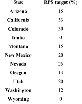
(25) 14. transmission capacity are grouped into 31 renewable hubs. I consider it is possible to construct up to four circuits of 500 kV to connect renewable hubs to the nearest high voltage buses (backbones) and up to 2 parallel circuit additions to existing corridors of 500 kV (interconnections). Finally, demand in each region is obtained by projecting the demand growth from 2004 to 2022. In the WECC representation, I include Baja California (Mexico), British Columbia and Alberta (Canada) and 11 US states (Arizona, California, Colorado, Idaho, Montana, Nevada, New Mexico, Oregon, Utah, Washington and Wyoming). Trading is allowed only among the US states. Although RPS goals vary on time, I used a static model that considers the RPS targets projected to year 2025 (Database of State Incentives for Renewable & Efficiency, 2013). In order to focus our analysis on the effects of REC trading, I do not consider the possibility of banking and/or borrowing RECs nor any specific RPS requirement on distributed generation. RPS goals are assumed to be those projected for the year 2025 as it is possible to see in Table 2. Table 1. RPS targets by state (Database of State Incentives for Renewable & Efficiency, 2013). State RPS target (%) Arizona. 15. California. 33. Colorado. 30. Idaho. 0. Montana. 15. New Mexico. 20. Nevada. 25. Oregon. 13. Utah. 20. Washington. 12. Wyoming. 0.

(26) 15. 3.2.Experiments Implemented in the WECC System Model. In this section, I describe how I quantify the benefits of allowing REC trading flexibility, measured as cost savings, CO2 emissions mitigation and energy price reductions. The REC trading flexibility is represented both by defining different-size trading regions and by considering different amounts of trading allowed. On one hand, I vary the fraction of the state-level RPS targets that is allowed to be imported from out of state, within certain region. Specifically, I analyze the effects of allowing REC imports up to 0%, 12.5%, 25%, 50%, 75% and 100% of the state RPS target from other states within certain region (this is, when satisfying up to that percentage of in-state RPS target with out-of-state renewable generation coming from certain region). I fixed a high noncompliance penalty, 500 [$/MWh], to ensure states would meet the RPS targets. This value is based on observed Solar RECs (SRECs) prices, so it represents an upper bound on the marginal cost of supplying power from renewable resources. On the other hand, I define different geographical eligibility limits and delivery requirements of RECs. Specifically, I define four scenarios that represent the geographical restrictions of trading among the WECC states, which are shown in Fig. 2. Although these geographical definitions attempt to capture some ideas of current REC trading constraints, the geographical restrictions actually existing are more complicated (e.g., some states restrict a fraction of the RECs that can come from certain other states), as explained below. These four scenarios are only intended to represent a range of flexibility in the geographical restrictions of REC trading from complete to none. Some states, as Colorado, do not have geographical restrictions on REC trading. Thus, they can comply with their RPS goals by importing RECs from any other state of the WECC. This situation is represented by the 1-Region scenario, in Fig 2a. I am especially interested in studying this scenario because it is an alternative under discussion by several policy makers in the US..

(27) 16. Some other states have geographical constraints on REC trading, obligating to the utilities to meet RPS goals with RECs generated in a specified region. Scenarios with 2, 3 and 4 regions, represented in Fig. 2b-d, show the alternatives analyzed in this work. The 2-Region scenario splits the WECC into two trading regions: the North and the South, where RECs can be freely traded only within each region. The 3-Region scenario adds a limit between the Pacific Northwest regions and the other Northern states. This limit attempt to illustrate situations like the one faced by Washington, which requires importing RECs only from Pacific Northwest states. Finally, the 4-Region scenario divides the WECC into four regions. Other states require complying with their RPS goals using partial in-state renewable generation. Partial in-state renewable generation can be represented by varying the amount of RECs allowed to import. As mentioned before, the effects of increasing REC trading flexibility are measured in terms of cost savings, CO2 emissions mitigation and energy price reductions. Cost indexes includes per-state costs and total system cost. Regarding CO2 emissions, I distinguish the effects on REC-importing and REC-exporting states. Regarding energy prices in the WECC, I computed the “average energy price” (. ) in each state by. calculating the quotient between the demand-weighed nodal energy price (i.e., the sum of the products between each nodal energy price and the nodal demand)2 and the total demand from the state (23). To compute the WECC system average price (. ), I. “weighted” the average energy price in each state using the total demand of each state (24).. 2. Nodal energy prices are computed as:. ∑. (. ). . This is, nodal prices correspond. to the changes in the objective function (O.F.) due to a 1-MWh variation in the load, which affects energy balance constraints, reserve margin requirement constraints, and RPSs constraints. Thus, nodal prices correspond to the sum over all constraints (C) of the partial derivative of the right-hand side (RHS) of the constraints multiplied by the respective demand. Since demand is a fixed quantity in our model, I create a variable, d b,h, in order to capture the effect of the changes in demand. Accordingly, I replaced the fixed parameter D b,h by the variable db,h in constraints (10), (17), (19) and (20) and I captured the effect in the objective function when 1 MWh changes in the load. This provides dual prices at each bus and hour..

(28) 17. ∑ ∑ ∑ ∑ All simulations were run using the AIMMS 3.13 optimization program and the CPLEX 12.4 solver on a computer with 4 cores and 4 GB of RAM.. (a). (b). (c). (d). Fig. 2. (a) 1-Region scenario: No Geographic Restrictions. (b) 2-Regions scenario. (c) 3-Regions scenario. (d) 4-Regions scenario..

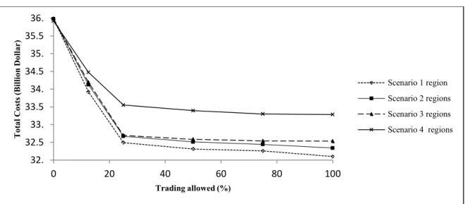
(29) 18. 4. RESULTS AND DISCUSSION. In the following subsections I analyze the results that I obtained with the model. I study how REC trading affects the total system cost, exports and imports of RECs by states, generation capacity investments, transmission investments, CO2 emissions and energy prices. 4.1. System Costs. I computed the total cost of the WECC, in the four geographically-constrained scenarios, as I varied the amount of REC trading (imports) allowed from 0% to 100%. Fig. 3 shows the results. If I compare the situation where full trading is allowed (100% REC trading allowed) and the case where no trading is allowed (0% REC trading allowed), in the 1-Region scenario, I observe from Fig. 3 that the total cost savings are $3.88 billion (10.79%). Interestingly, the total cost reduction is significantly large even when allowing a relatively small level of REC trading. Specifically, the total cost decreases by $3.49 billion (9.69% cost savings) when I only allow up to 25% of RECs at state level being imported from any other state belonging to the WECC. It is remarkable the knee observed in Fig. 3 at 25% of REC trading allowed. There are two facts that cause this knee. Firstly, as the first 25% of REC flexibility is allowed, the best renewable resources in the WECC are used. Allowing further REC trading yields to the use of additional, less efficient, renewable resources in the WECC, implying that the total cost is reduced at a lower rate. Secondly, as REC flexibility is increased, transmission lines become more congested and, thus, not all desirable REC trading is physically feasible (unless more transmission investments are made). This suggests that it is also interesting to analyze the transmission investment costs jointly with the total costs. I dedicate a subsection to study transmission investments later on. From Fig. 3, it is also remarkable that total cost is similar in the 1-Region, 2-Regions and 3-Regions scenarios. Naturally, when imposing more geographical constraints (going from 1-Region to 4-Region scenarios) the exchange of renewable energy is.

(30) 19. limited to only states that belong to the same region and, thus, the total cost increases. However, the difference between the 4-Regions scenario and the rest of scenarios (the total cost difference in the 1-Region scenario and the 4-Regions scenario is $1.19 billion (3.6%) when allowing 100% REC trading) suggests that the total cost is very sensitive to the way geographical constraints are defined. Particularly, the total cost in the 4-Regions scenario is significantly larger than in the other scenarios because this scenario prevents California from taking advantage of good renewable resources located in states like Utah, Colorado and New Mexico. In fact, when imposing the 4-Regions scenario, California is forced to import RECs from Nevada and Arizona, which are not net REC exporters in the other scenarios. The costs for all scenarios are shown in Appendix A on Tables A.1, A.2, A.3 and A.4. In summary, results show that trading RECs among states has positive effects on the WECC system cost. To obtain significant cost savings it is enough to allow a relatively small level of REC trading (such as up to 25%) and to design smart geographic configurations that promote renewable generation in states. .. Total Costs (Billion Dollar). 36. 35.5. 35. 34.5 Scenario 1 region. 34.. Scenario 2 regions. 33.5. Scenario 3 regions. 33.. Scenario 4 regions. 32.5 32. 0. 20. 40. 60. 80. 100. Trading allowed (%). Fig. 3: Total Cost as a Function of Trading Flexibility..

(31) 20. 4.2.Trading of REC. When REC trading is allowed, states that generate more renewable energy than the local RPS target are able to sell RECs to states that fall short of their RPS targets. On the contrary, when REC trading is not allowed, all states meet their RPS targets with instate renewable generation. Recall from Section 4 that I consider a high noncompliance penalty (500 $/MWh, based on observed Solar RECs prices), so RPS goals are always met. Fig. 4 shows REC transactions for different scenarios. Appendix B shows in Table B.1, B.2, B.3 and B.4 the renewable energy generation and the required demand of renewable energy for each of the cases in study. The sizes of the bars represent the magnitudes of the exports (white bars) and imports (dark bars) of RECs. The fraction of the state’s demand that is exported or imported by the state is shown in Fig.4 as a percentage. For instance, in Fig. 4a, the size of the California’s bar corresponds to 29 GWh per year of renewable energy imported, which represents 8.3% of the demand in California. In the case of the 1-Region scenario and allowing either 25% or 100% of REC trading (Fig. 4a and 4b), the states that export RECs are Idaho, New Mexico, Montana, Utah, and Wyoming and the states that import RECs are Arizona, California, Colorado, Nevada, and Washington. Oregon either exports or imports RECs depending on the REC trading flexibility that is allowed. An interesting outcome is that Idaho and Wyoming export RECs (when allowed) although they do not have RPS targets. This is because these states have cheap renewable resources that are highly valuable by other states having RPS obligations. The number of exporting states varies depending on the geographic trading configurations. For instance, looking at the states selling RECs when 25% of REC flexibility is allowed, I obtain that 5 states export RECs in the 1-Region scenario, 6 states export RECs in the 2-Regions scenario, 5 states export RECs in the 3-Regions scenario, and 7 states export RECs in the 4-Regions scenario. Several facts explain these.

(32) 21. changes. For example, when 25% of REC trading is allowed in the 2-Regions scenario (Fig. 4c), Colorado becomes an exporting state, producing more renewable energy than in the 1-Region scenario (with the same REC trading flexibility). Also, when 25% of REC trading is allowed in the 3-Regions scenario (Fig. 4d), Montana becomes an importing state. And, when 25% of REC trading is allowed in the 4-Regions scenario, 7 states export RECs due to the more strict geographical constraints. Consequently, the way geographical restrictions of REC trading are defined has important effects on REC trading.. (a). (c). (b). (d).

(33) 22. Fig. 4: REC exports (white bars) and imports (gray bars) in the following cases: (a) 25% of REC trading is allowed in the 1-Region scenario, (b) 100% of REC trading is allowed in the 1-Region scenario, (c) 25% of REC trading is allowed in the 2-Regions scenario, and (d) 25% of REC trading is allowed in the 3-Regions scenario. For other levels of REC flexibility, I observe a similar REC trading behavior. Precisely, exports and imports of RECs vary considerably depending on the REC trading flexibility allowed when allowing up to 25% of REC trading, while exports and imports of RECs do not significantly vary when more than 25% of REC trading is allowed.. 4.3. Generation Capacity Investments. It is interesting to study the changes in the generation expansion investments by technology as REC trading flexibility varies. It is important to mention that, in this analysis, I only focus on new generation capacity investments. Accordingly, I do not analyze the current generation mix in the WECC. Moreover, recall that, following the new standards of the United States Environmental Protection Agency (US EPA), I do not allow the construction of new coal power plants without CCS technologies, new large hydro power plants and new nuclear power plants. Fig. 5 shows the distribution of the generation capacity investments by technology in the 1-Region scenario both in the case when no REC trading is allowed (Fig. 5a) and in the case when 100% REC trading is allowed (Fig. 5b). A quick observation of Fig. 5 reveals that no new coal power plants are built. This is due to the high capital cost of coal power plants with CCS technologies. In general terms, the investment level in new renewable generation capacity is larger when no REC trading is allowed. This is obviously a consequence of forbidding REC trading flexibility, which imposes an obligation to each state of meeting its RPS goal using only in-state renewable resources (although some cheaper renewable resources.

(34) 23. located at other states are not used yet). Regarding this fact, states like Wyoming and Idaho, which have cheap renewable resources and do not have RPSs obligations, would only invest in large amounts of renewable generation capacity when REC trading flexibility is allowed. When there is no flexibility on RECs trading (Fig. 5a), the investments in solar generation represent a 31% of the generation investments. This is because states like California have strict RPS goals and do not have extensive cheap renewable resources (so, they need to invest in in-state solar generation capacity to meet their RPS targets). When full REC trading flexibility is allowed in the WECC (Fig. 5b), the investments in solar generation decrease significantly and they are replaced by out-of-state cheaper renewable technologies located within the WECC.. Biomass 3%. Hydro 12%. Gas 20%. Biomass 3%. Hydro 15%. Gas 26%. Geother mal 4%. Wind 30%. Solar 31%. (a). Geotherm al Solar 6% 6%. Wind 44%. (b). Fig. 5: Generation investments by technology in the 1-Region scenario, when (a) no REC trading is allowed, and when (b) 100% of REC trading flexibility is allowed. In the following subsections, I analyze how REC trading affects transmission investments, CO2 emissions and energy prices, focusing on the effects in three particular states that have different positions in the REC market. These include California, which is a REC-importing state, New Mexico, a REC-exporting state, and Wyoming, which has no RPS obligation..

(35) 24. 4.4. Transmission Investments. One might expect that more renewable energy trade would imply more total energy trade and, thus, more need for transmission investments. However, this is not necessary the case, as I show here. Fig. 6 shows the aggregate transmission investment cost as a function of the REC trading allowed in the WECC. As observed in Fig. 6, transmission investment costs are very sensitive to the exact REC flexibility allowed. One of the reasons for this is that transmissions investment costs represent a small fraction of the total costs (annualized transmission investment costs vary between 0.4 and 0.9 billion of dollars while total system costs vary between 32 and 36 billion of dollars). Another reason for this fact is the lumpiness of transmission investments (i.e., transmission investment variables in the model are binary). The lumpy characteristic of transmission investments leads to unpredictable investment patterns, which prevent us from ensuring a correlation between the gains from REC trading and the transmission investment costs (Indeed, when considering continuous transmission investment variables in the model, this non-monotonicity observed in Fig. 6 disappears). Even though transmissions investment costs represent a small fraction of the total costs and the lumpiness of transmission investments leads to unpredictable investment patterns, it is still surprising that transmission investments do not have a correlation with the REC trading allowed. This fact highlights the importance of jointly studying renewable energy integration and transmission planning, in contrast with common practice of analyzing them in an isolated manner..

(36) 25. Transmission Investment Costs (Billion Dolar). 1 0.9 0.8 0.7. Scenario 1 region. 0.6. Scenario 2 regions Scenario 3 regions. 0.5. Scenario 4 regions. 0.4 0.3 0. 20. 40. 60. 80. 100. Trading allowed (%). Fig. 6: Aggregate transmission investment cost versus the percentage of trading allowed.. Fig. 7 shows the transmission investment costs in California, New Mexico and Wyoming in the 1-Region scenario. For new transmission lines connecting two states, I equally split transmission investment costs. As previously mentioned, the lumpy characteristic of transmission investments leads to unpredictable investment patterns in each state. In California, the transmission investment cost increases when allowing either between 0 and 12.5% of REC trading flexibility or between 50% and 75% of REC trading flexibility. This is consistent with a lower level of solar generation investments in California in these ranges. In Wyoming and New Mexico, the transmission investment costs increase more substantially only when allowing between 50% and 75% of REC trading flexibility. This is mainly due to the REC exporting possibilities of these states..

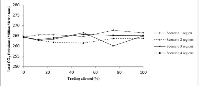
(37) Transmission Investment Costs (Billion Dollar). 26. 0.3. 0.2 California New Mexico. 0.1. Wyoming. 0 0. 20. 40. 60. 80. 100. Trading allowed (%). Fig. 7: Transmission investment costs per state in the 1-Region scenario.. It is interesting to mention that, consistent with the findings in (Munoz et al., 2013a), I found that the transmission lines constructed in different solutions (i.e., when considering different levels of REC trading allowed) are not necessarily subsets of each other. For example, the portfolio of lines in which California invests when 25% of REC trading flexibility is allowed is not a subset of the portfolio of lines in which California invests when 50% or 75% of REC trading flexibility is allowed. This fact suggests, among other things, that enforcing RPS goals year by year might lead to suboptimal transmission investments. 4.5. CO2 Emissions. Fig. 8 shows the total amount of CO2 emissions in the WECC as a function of the REC trading allowed. Details are shown in Appendix C on Table C.1. When no REC trading is allowed, total CO2 emissions are 264.3 millions of metric tons. When increasing REC trading flexibility, CO2 emissions stay relatively constant, as it can be.

(38) 27. seen in Fig. 8. That is, additional REC trading does not significantly either help or hurt the environment, in terms of CO2 emissions. Intuitively, by importing RECs, a state may make up for that generation with conventional generation from either the same state or other states, which would increase CO2 emissions. On the other hand, these increments in CO2 emissions would be compensated partially or completely by the CO2 emission reductions in states generating more renewable power in order to export RECs. Consequently, as REC trading flexibility is increased, it is not evident the way conventional and renewable generators are dispatched and, thus, the way CO2 emissions behave. Moreover, as mentioned before, the lumpy characteristic of transmission investments affects generation. Total CO2 Emissions (Million Metric tons). investments and operations, making CO2 emissions even more unpredictable.. 280 275 270 Scenario 1 region. 265. Scenario 2 regions. 260. Scenario 3 regions Scenario 4 regions. 255 250 0. 20. 40. 60. 80. 100. Trading allowed (%). Fig. 8: Aggregate WECC CO2 emissions as a function of the REC trading allowed. Fig. 9 shows the amount of CO2 emissions in some states of the WECC as a function of the REC trading allowed. In the case of California, as shown in Fig. 9, CO2 emissions decrease when allowing either between 0 and 12.5% of REC trading flexibility or between 50% and 75% of REC trading flexibility. Note that the transmission investment cost increases in the same ranges of REC trading flexibility (Fig. 7), which suggests that.

(39) 28. more transmission investments leads to more REC imports and, thus, to less CO2 emissions. However, this is not easily generalizable due to the possibility of having a CO2 leakage effect, as shown in (Sauma, 2012b). In fact, California simultaneously imports RECs and decreases solar generation when allowing REC trading, which makes difficult to predict the magnitude of the CO2 leakage effect in an ex-ante manner. On the other hand, Wyoming, which does not have a RPS obligation, would invest in solar and wind power generation as REC trading is allowed and it would sell the resulting RECs to other states. Note that, in the case of Wyoming, the transmission investment cost increases when allowing either between 0 and 12.5% or between 50% and 75% of REC trading flexibility (Fig. 7), but CO2 emissions tend to increase in the same ranges of REC trading flexibility (Fig.9). This makes evident the unpredictability of the magnitude of the CO2 leakage effect I just mentioned. In the case of New Mexico, wind and solar power generation increase when REC trading flexibility is increased, making New Mexico a REC-exporting state. When 12.5% and 25% of REC trading flexibility are allowed, CO2 emissions slightly decrease due to the reduction in the local use of coal and natural gas to generate power. In contrast, between 50% and 75% of REC trading flexibility, coal power generation increases and natural gas power generation remains constant, leading to a net increase in. CO2 Emissions (Million Metric tons). the CO2 emissions. 70 60 50 California. 40. New Mexico Wyoming. 30 20 0. 20. 40. 60. 80. 100. Trading Allowed (%). Fig. 9: CO2 emissions per state in the 1-Region scenario..

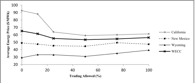
(40) 29. 5.6 Energy Prices Fig. 10 shows the “average energy price” in the WECC and in some states of the WECC as a function of the REC trading allowed, in the 1-Region scenario. Results are similar for the other three scenarios. The average energy price in each state is computed by calculating the quotient between the demand-weighed nodal energy price (i.e., the sum of the products between each nodal energy price and the nodal demand) and the total demand from the state. To compute the WECC system average price, I “weighted” the average energy price in each state using the total demand of each state. Recall from Section 3 that nodal energy prices correspond to the changes in the total system cost due to a 1-MWh variation in the load, which affects energy balance constraints, reserve margin requirement constraints, and RPSs constraints. As I increase REC trading flexibility, the average energy price in the WECC is generally lower than when REC trading is forbidden. However, the situation significantly varies by state. In California, energy prices decrease as more REC trading is allowed, while energy prices tend to increase in Wyoming. To explain these differences, I present in Fig. 11 the in-state REC generation as a function of the REC trading allowed, in the 1-Region scenario. Average energy prices in California decrease as more REC trading is allowed mainly because the more REC trading is allowed, the less in-state solar RECs are generated in California, as seen in Fig.11. Since solar RECs are more expensive than other RECs, allowing California to import RECs from other states (instead of producing in-state solar RECs) leads to an average energy price reduction. In contrast, average energy prices in Wyoming tend to increase as REC trading flexibility increases. This occurs because Wyoming, a REC-exporting state, increases solar RECs generation, as more REC trading is allowed, as seen in Fig. 11. At the same time, Wyoming increase coal power generation (CO2 leakage effect) as more REC trading is allowed, which also contributes to raise the energy price..

(41) 30. In the case of New Mexico, average energy prices stay relatively constant as REC trading flexibility increases. This is because this REC-exporting state generates RECs mainly from wind and biomass resources (not using more expensive in-state RECs such as solar RECs).. Average Energy Price ($/MWh). 100 90 80. 70 California. 60. New Mexico. 50. Wyoming. 40. WECC. 30 20 0. 20. 40. 60. 80. 100. Trading Allowed (%). Fig. 10: Average energy prices in the WECC and per state in the 1-Region scenario.. In- state REC Generation (GWh-year). 60,000 50,000 40,000 Solar CA. 30,000. Wind CA Wind NM. 20,000. Solar WY. 10,000 0 0. 20. 40. 60. 80. 100. 120. Trading allowed (%). Fig.11: In-state REC generation by technology and state, in the 1-Region scenario..

(42) 31. 6. CONCLUSIONS. I quantify the benefits of allowing increased trade of RECs among the states belonging to the WECC in order to meet state RPSs. The results show that if I increase the amount of RECs traded among states, the total cost decreases. Remarkably, the cost reduction is significantly large even for a relatively small level of trade. In particular, the total cost decreases by 9.69% when I allow 25% of RECs at state level being imported from any other state belonging to the WECC. When allowing even more trade, the total cost continues decreasing, but at a lower rate. Results also suggest that increasing REC trading flexibility does not necessarily imply an increase in the optimal transmission investment costs (and, thus, does not necessarily imply an increase in the environmental damage from building transmission lines). As well, increasing REC trading flexibility does not seem to have a significant impact on CO2 emissions and/or energy prices. All our results are obtained using a power transmission expansion planning model, formulated as a mixed integer program, which minimizes the annualized investment and operations costs of the WECC system for year 2022. The model uses a 240 bus representation of the WECC network and incorporates the indivisibility property of transmission investments, the variability of renewable resources, energy balance constraints, Kirchhoff´s current and voltage laws, transmission capacity constraints, generation capacity constraints, generation investment constraints, reserve margin requirement constraints, flowgate constraints, and RPS constraints, among other features that reflect the physics and economics of power systems. I created four scenarios which represented four different configurations of geographic restrictions. For each scenario I compared the results while I varied the allowed trading of RECs among states. I showed that as the geographical restrictions for REC trading are increased, the total system costs increase. However, the total costs were relatively similar when imposing the 1-Region, the 2-Regions, or the 3-Regions scenarios. In the 4-Regions scenario, a much larger system cost resulted because this.

(43) 32. scenario prevents California from taking advantage of good renewable resources located in states like Utah, Colorado and New Mexico. This suggests that, in order to reduce the implementation costs of RPS policies, authorities should not only allow more REC trading flexibility, but also design smart geographic configurations that promote renewable generation. Increased REC trading flexibility allows meeting RPSs in a more cost-efficient manner. Allowing more REC trading flexibility encourage that states like Idaho and Wyoming, which have cheap renewable resources and do not have RPS targets, invest more in renewable energy and export RECs to other states with RPS obligations. Intuitively, one might expect a tradeoff between the cost gains from REC trade and the transmission investment cost. However, this is not always evident. Both the fact that transmissions investment costs represent a small fraction of the total costs and the lumpy characteristic of transmission investments leads to unpredictable transmission investment patterns, which prevent us from ensuring a correlation between the gains from REC trading and the transmission investment costs. This fact highlights the importance of jointly studying renewable energy integration and transmission planning, in contrast with common practice of analyzing them in an isolated manner. As well, it is not evident the way CO2 emissions behave as REC trading flexibility is increased. The total system emissions remain relatively constant in the four scenarios considered. Again, the fact that transmissions investment costs represent a small fraction of the total costs and the lumpy characteristic of transmission investments affects the way conventional and renewable generators are dispatched and, thus, affects generation investments and operations. This makes that CO2 emissions are sensitive to the precise REC trading flexibility allowed, as this affects the power system dispatch. Our results suggest that the average energy price in the whole WECC would slightly decrease as more REC trading is allowed. However, average energy prices in some states would increase. For example, average energy prices in Wyoming tend to increase as REC trading flexibility increases mainly because Wyoming increases both solar RECs generation and coal power generation (CO2 leakage effect) as more REC trading is.

(44) 33. allowed. In California, average energy prices decrease as more REC trading is allowed, mainly because the more REC trading is allowed, the less in-state solar RECs are generated in California. There are several routes for future work associated with this research. Firstly, it would be interesting to see a similar study considering all the states of the US, or even considering different countries with different RPS goals located within a region (like the European Union). Secondly, it would be interesting to study the interaction between RPS targets and energy efficiency goals, analyzing the effects of including new eligible technologies. Finally, future research may also focus on the development of optimal methods for choosing adequate geographic restrictions for REC trading..

(45) 34. REFERENCES Alguacil, N., Motto, A., Conejo, A., 2003. Transmission expansion planning: A mixedinteger LP approach. IEEE Transactions on Power Systems 18(3), 1070-1077. Barry, D, 2002. The market for tradable renewable energy credits. Ecological Economics, 42(3), 369-379. Berendt, C., 2006. A State-Based Approach to Building a Liquid National Market for Renewable Energy Certificates: The REC-EX Model. The Electricity Journal 19(5), 5468. Castle, S., 2014. Europe, facing economic pain, may ease climate rules. NY Times, Available. online. on. http://www.nytimes.com/2014/01/23/business/international/. [Accessed on January 23, 2014]. Cory, K., Swezey, B., 2007. Renewable portfolio standards in the states: balancing goals and implementation strategies, NREL Report No. TP-640-41409. Available online on http://www.nrel.gov/docs/fy08osti/41409.pdf. [Accessed on December 10, 2013]. de la Torre, S., Conejo, A., Contreras, J., 2008. Transmission expansion planning in electricity markets. IEEE Transactions on Power Systems 23(1), 238-248. Elder, B., 2007. Renewable energy credits (RECs) in California. Status after passage of Senate Bill 107 of 2006. University of San Diego School of Law. Available online on http://www.nrel.gov/docs/fy08osti/41409.pdf. [Accessed on December 18, 2013]..

(46) 35. Fischer, C., Newell, R., 2008. Environmental and technology policies for climate mitigation. Journal of Environmental Economics and Management 55, 142–162. Heeter, J., Bird, L., 2011. Status and trends in US compliance and voluntary renewable energy certificate markets (2010 data). NREL Report No. TP-6A20-52925. Available online on http://www.nrel.gov/docs/fy12osti/52925.pdf [Accessed on December 6, 2013]. Holt, E., Wiser, R., 2007. The treatment of renewable energy certificates, emissions allowances, and green power programs in state renewables portfolio standards. Report LBNL. No.. 62574.. Available. online. http://emp.lbl.gov/sites/all/files/REPORT%20lbnl%20-%2062574.pdf. [Accessed. on on. November 22, 2013]. Kung, H., 2012. Impact of deployment of renewable portfolio standard on the electricity price in the State of Illinois and implications on policies. Energy Policy 44, 425-430. Mack, J., Gianbecchio, N., Campopiano, M., Logan, S., 2011. All RECs are local: How in-state generation requirements adversely affect development of a robust REC market. The Electricity Journal 24(4), 8-25. Mozumder, P., Marathe, A, 2004. Gains from an integrated market for tradable renewable energy credits (TRECs). Ecological Economics 49(3), 259-272. Muñoz, C., Sauma, E., Contreras, J., Aguado, J., de la Torre, S., 2012. Impact of high wind power penetration on transmission network expansion planning. IET Generation, Transmission & Distribution 6(12), 1281-1291..

(47) 36. Munoz, F., Sauma, E., Hobbs, F., 2013a. Approximations in power transmission planning: implications for the cost and performance of renewable portfolio standards. Journal of Regulatory Economics 43(3), 305-338. Munoz, F., Hobbs, B., Ho, J., Kasina, S., 2013b. An engineering-economic approach to transmission planning under market and regulatory uncertainties: WECC case study. IEEE Transactions on Power Systems 29(1), 307-317. National Renewable Energy Laboratory (NREL), 2012a. Western Wind Resources Dataset. Available online on: http://wind.nrel.gov/Web_nrel/ [Accessed on October 6, 2013]. National Renewable Energy Laboratory (NREL), 2012b. Renewable Resources Data Center – PVWatts. Available online on: http://www.nrel.gov/rredc/pvwatts/ [Accessed on October 6, 2013]. Pozo, D., Sauma, E. E., and Contreras, J., 2013. A Three-Level Static MILP Model for Generation and Transmission Expansion Planning. IEEE Transactions on Power Systems 28(1), 202-210. Price, J., Goodin, J., 2011. Reduced Network Modeling of WECC as a Market Design Prototype. Proceedings of the IEEE Power and Energy Society General Meeting. Sauma, E., 2012a. Policies for encouraging non-conventional renewable energy in Chile (Políticas de fomento a las energías renovables no convencionales (ERNC) en Chile). Pontificia Universidad Católica de Chile. Report N. 52, available online on http://politicaspublicas.uc.cl/publicaciones/ver_publicacion/3 [Accessed on January 12, 2014]..

(48) 37. Sauma, E., 2012b. The impact of transmission constraints on the emissions leakage under cap-and-trade program. Energy Policy 51, 164-171. Sauma, E., Oren, S., 2006. Proactive planning and valuation of transmission investments in restructured electricity markets. Journal of Regulatory Economics 30(3), 261-290. Sauma, E., Oren, S., 2007. Economic criteria for planning transmission investment in restructured electricity markets. IEEE Transactions on Power Systems 22(4), 1394-1405. U.S. Database of State Incentives for Renewables and Efficiency (US DSIRE), 2013. Summary maps, available online on http://www.dsireusa.org/. [Accessed on January 24, 2014]. U.S. Energy Information Administration, 2012. Capital costs estimates for electricity generation plants, available online on: http://www.eia.gov/oiaf/beck_plantcosts. [Accessed on January 30, 2014]. Vajjhala, S. P., Paul, A., Sweeney, R., Palmer, K, 2008. Green corridors: Linking interregional transmission expansion and renewable energy policies. Discussion Paper 08/06. Washington, DC: Resources for the Future. Villasana, R. , Garver, L., Salon, S., 1985. Transmission network planning using linear programming. IEEE Transactions on Power Apparatus and Systems 2, 349-356. Wiser, R., Namovicz,C., Gielecki,M., Smith R., 2007. The experience with renewable portfolio standards in the United States. The Electricity Journal 20(4), 8-20..

(49) 38. APPENDICES.

(50) 39. APPENDIX A. COSTS OF THE SYSTEM Table A. 1. Investments and operating costs (Billion dollar) versus trading allowed (%). Scenario 2. Trading. Investments Costs. Operating Costs. Total Costs. allowed (%). (Billion dollar). (Billion dollar). (Billion dollar). 0. 18.94. 17.04. 35.98. 12.5. 17.21. 16.71. 34.92. 25. 15.74. 16.75. 32.49. 50. 15.34. 16.98. 32.31. 75. 15.41. 16.84. 32.26. 100. 15.12. 16.98. 32.09. Table A. 2. Investments and operating costs (Billion dollar) versus trading allowed (%). Scenario 2. Trading. Investments Costs. Operating Costs. Total Costs. allowed (%). (Billion dollar). (Billion dollar). (Billion dollar). 0. 18.94. 17.04. 35.98. 12.5. 17.45. 16.68. 34.13. 25. 15.61. 17.06. 32.67. 50. 15.53. 16.98. 32.51. 75. 15.65. 16.79. 32.44. 100. 15.66. 16.68. 32.34.

(51) 40. Table A. 3. Investments and operating costs (Billion dollar) versus trading allowed (%). Scenario 3. Trading. Investments Costs. Operating Costs. Total Costs. allowed (%). (Billion dollar). (Billion dollar). (Billion dollar). 0. 18.94. 17.04. 35.98. 12.5. 17.15. 17.04. 34.19. 25. 15.75. 16.95. 32.69. 50. 15.57. 17.01. 32.58. 75. 15.41. 17.13. 32.54. 100. 15.59. 16.94. 32.53. Table A. 4. Investments and operating costs (Billion dollar) versus trading allowed (%). Scenario 4. Trading. Investments Costs. Operating Costs. Total Costs. allowed (%). (Billion dollar). (Billion dollar). (Billion dollar). 0. 18.94. 17.04. 35.98. 12.5. 17.56. 16.92. 34.47. 25. 16.39. 17.17. 33.55. 50. 16.38. 17.02. 33.39. 75. 16.21. 17.09. 33.29. 100. 16.48. 16.81. 33.29.

(52) 41. APPENDIX B. RENEWABLE GENERATION Table B. 1. Renewable generation (GWh-year) and required demand. Exporting and importing states in Scenario 1 for 25% of flexibility. State. Renewable generation. Required demand. Export/Import. (GWh-year). (GWh-year). (GWh-year). Arizona. 13,443.25. 16,665.40. -3,222.16. California. 86,855.12. 115,806.83. -28,951.71. Colorado. 13,902.82. 18,537.09. -4,634.27. Montana. 4,682.17. 2,853.29. 1,828.87. New Mexico. 31,023.64. 4,338.48. 26,685.17. Nevada. 13,915.17. 17,317.55. -3,402.38. Oregon. 13,917.24. 14,143.34. -226.01. Utah. 8,005.33. 7,782.52. 222.81. Washington. 11,732.60. 15,643.46. -3,910.87. Idaho. 3,208.13. 0. 3,208.13. Wyoming. 12,402.50. 0. 12,402.50.

(53) 42. Table B. 2. Renewable generation (GWh-year) and required demand. Exporting and importing states in Scenario 1 for 100% of flexibility. State Arizona California Colorado Montana New Mexico Nevada Oregon Utah Washington Idaho Wyoming. Renewable generation. Required demand. Export/Import. (GWh-year). (GWh-year). (GWh-year). 15,521.36. 16,665.41. -1,144.05. 79,736.71. 115,806.83. -36,070.12. 4,425.55. 18,537.09. -14,111.54. 19,403.01. 2,853.29. 16,549.72. 31,573.60. 4,338.48. 27,235.12. 13,915.17. 17,317.55. -3,402.38. 16,421.71. 14,143.34. 2,278.37. 8,031.61. 7,782.51. 249.09. 5,326.96. 15,643.46. -10,316.51. 6,329.80. 0. 6,329.80. 12,402.50. 0. 12,402.50.

(54) 43. Table B. 3. Renewable generation (GWh-year) and required demand. Exporting and importing states in Scenario 2 for 25% of flexibility. State Arizona California Colorado Montana New Mexico Nevada Oregon Utah Washington Idaho Wyoming. Renewable generation. Required demand. Export/Import. (GWh-year). (GWh-year). (GWh-year). 15,521.36. 16,665.41. -1,144.05. 86,855.12. 115,806.83. -28,951.71. 20,564.07. 18,537.09. 2,026.98. 4,057.13. 2,853.29. 1,203.84. 34,494.75. 4,338.48. 30,156.27. 14,980.96. 17,317.55. -2,336.59. 11,794.49. 14,143.34. -2,348.85. 8,031.61. 7,782.51. 249.09. 11,732.60. 15,643.46. -3,910.87. 4,141.20. 0. 4,141.20. 914.67. 0. 914.67.

(55) 44. Table B.4. Renewable generation (GWh-year) and required demand. Exporting and importing states in Scenario 3 for 25% of flexibility. State Arizona California Colorado Montana New Mexico Nevada Oregon Utah Washington Idaho Wyoming. Renewable generation. Required demand. Export/Import. (GWh-year). (GWh-year). (GWh-year). 15,521.36. 16,665.41. -1,144.05. 86,855.12. 115,806.83. -28,951.71. 24,366.91. 18,537.09. 5,829.81. 2,139.97. 2,853.29. -713.32. 31,573.60. 4,338.48. 27,235.12. 14,099.28. 17,317.55. -3,218.27. 12,578.17. 14,143.34. -1,565.17. 8,031.61. 7,782.51. 249.09. 11,732.60. 15,643.46. -3,910.87. 5,476.04. 0. 5,476.04. 914.67. 0. 914.67.

(56) 45. APPENDIX C.EMISSIONS Table C. 1. Emissions (Million metric tons of CO2) in California, New Mexico and Wyoming. Scenario 1. State. Emissions (Million Metric tons of CO2) Trading Allowed 0%. California New Mexico Wyoming. 12.5%. 25%. 50%. 62.87046 48.67163 66.38915 61.55531. 75%. 100%. 50.6913 61.47374. 38.50534 38.59201 35.31094 36.09141 37.73262 36.21241 26.33811 29.34057 29.07121. 26.4871 27.91685 28.24726.

(57)