Photonic Information Processing

Texto completo

(1)DOCTORAL THESIS 2018 Doctoral Program of Physics PHOTONIC INFORMATION PROCESSING. Julián Bueno Moragues.

(2) 2.

(3) DOCTORAL THESIS 2018 Doctoral Program of Physics PHOTONIC INFORMATION PROCESSING Julián Bueno Moragues. Director: Ingo Fischer Director: Daniel Brunner Tutor: Pere Colet Doctor by the Universitat de les Illes Balears.

(4) 2.

(5)

(6) 2.

(7) Abstract Abstract of the thesis In the current thesis we experimentally study the dynamics of complex photonic systems including semiconductor laser systems with delayed feedback and spatially coupled optical systems, and employ their dynamics for information processing. Photonic delay systems offer a broad range of complex dynamics, making them excellent testbeds for the study of nonlinear dynamics. We take advantage of the complex dynamics and turn the photonic delay systems into information processing systems by applying techniques from the field of neural networks, studying their properties, and demonstrating successful performance. First we study the dynamics of a semiconductor laser with two delayed optical feedbacks. The temporal evolution of the intensity from the laser is represented and studied in a two dimensional pseudo-space, which conveniently allows to visualize structures in the dynamics. Two dynamical regimes are being addressed in this study, Spiral Phase Defects and Defect-mediated Turbulence. Spiral Phase Defects that were predicted for this system have not been observed, and we discuss the possible reasons. Defect-mediated Turbulence is observed in a broad range of parameters. The defect-mediated dynamics is analyzed in detail by using intensity distribution and spectral analysis. The spectral analysis shows an exponential decay of the spectra for low bias currents of the semiconductor laser. For increasing bias currents, the spectra exhibit a double power law decay that merges into a single power law as the bias currents is increased. This indicates a scale-free behavior in the dynamics for high bias currents. Next, we study the use of a semiconductor laser with a single delay optical feedback and optical injection as a delay-based reservoir computer. We study the fundamental properties of the system, specifically the properties of injection locking, consistency, and memory. We evaluate the performance of the system in a prediction task, and link the 3.

(8) different properties to performance. The impact of crucial experimental parameters on the properties are evaluated, and the implications discussed. Moreover, we explore further functionalities. Suitable properties and good performance are demonstrated for injection at modulation rates up to to 20 GSa/s, and also for optical injection detuned hundreds of GHz from the solitary emission of the semiconductor laser. Furthermore, we demonstrate how to create a reservoir with nodes with different sets of properties, and show that performance in a prediction task can be improved with this approach. In the final part, we design and build a spatially extended reservoir computer with 900 coupled nonlinear nodes. The reservoir is implemented with a Spatial Light Modulator (SLM), and the nonlinearity is realized by taking advantage of the polarization modulation of the Spatial Light Modulator (SLM) together with a Polarization Beam Splitter (PBS). The coupling in the network is experimentally implemented with a Diffractive Optical Element (DOE), resulting in coupling beyond first neighbors. The input layer is implemented digitally employing the control computer. The output layer is experimentally implemented with a Digital Micro-mirror Display (DMD) and a lens, where the configuration of the Digital Micro-mirror Display (DMD) determines the values of the output weights in the reservoir computer. We evaluate the dynamics of the nodes and demonstrate suitable nonlinear dynamics in the network. Learning rules are implemented to allow the system to autonomously change the output weights based on previous performance, and to search for an optimized configuration attaining low errors in specific tasks. We demonstrate successful operation of the reservoir computer by showing that, despite some limitations, it is capable of learning reducing the error in a prediction task and finally exhibiting very low prediction errors.. Resumen de la tesis En la presente tesis estudiamos experimentalmente la dinámica de sistemas fotónicos complejos que incluyen sistemas de láser semiconductor con retroalimentación retardada y sistemas ópticos acoplados espacialmente, y empleamos sus dinámicas para el procesamiento de la información. Los sistemas de retardo fotónico ofrecen una amplia gama de dinámicas complejas, lo que los convierte en excelentes bancos de pruebas para el estudio de dinámicas no lineales. Nosotros aprovechamos las dinámicas complejas y convertimos los sistemas fotónicos con retardo en sistemas de procesamiento de información aplicando técnicas del campo 4.

(9) de las redes neuronales, estudiando sus propiedades, y demostrando el desempeño exitoso. Primero, estudiamos la dinámica de un láser semiconductor con dos retroalimentaciones ópticas retardadas. La evolución temporal de la intensidad del láser es representada y estudiada en un pseudoespacio bidimensional, que convenientemente permite visualizar estructuras en la dinámica. Dos regı́menes dinámicos han sido abordados en este estudio, Spiral Phase Defects y Defect-mediated Turbulence. Spiral Phase Defects que se predijeron para este sistema no se han observado, y discutimos las posibles razones. Defect-mediated Turbulence es observado en un amplio rango de parámetros. La dinámica mediada por defectos es analizada en detalle mediante el uso de la distribución de intensidad y el análisis espectral. El análisis espectral muestra un decaimiento exponencial de los espectros para bajas corrientes eléctricas del láser semiconductor. Para corrientes eléctricas más altas, los espectros muestran dos decaimientos potenciales que se fusiona en una ley de potencia única a medida que se incrementan las corrientes eléctricas. Esto indica un comportamiento sin escalas en las dinámicas para altas corrientes eléctricas. A continuación, estudiamos el uso de un láser semiconductor con una única retroalimentación óptica retardada y una inyección óptica como un ordenador de reservorio basada en el retardo. Estudiamos las propiedades fundamentales del sistema, especı́ficamente las propiedades de bloqueo de inyección, la consistencia, y la memoria. Evaluamos el rendimiento del sistema en una tarea de predicción y vinculamos las diferentes propiedades con el rendimiento. El impacto de parámetros experimentales cruciales en las propiedades es evaluado, y las implicaciones son analizadas. Por otra parte, exploramos otras funcionalidades. Propiedades adecuadas y buen rendimiento son demuestrados para inyección a tasas de modulación de hasta 20 GSa/s, y también para inyección óptica sintonizada a cientos de GHz de la emisión solitaria del láser semiconductor. Además, demostramos cómo crear un reservorio con nodos con diferentes conjuntos de propiedades, y mostramos que el rendimiento en una tarea de predicción se puede mejorar con esta estrategia. En la parte final, diseñamos y construimos un ordenador de reservorio espacialmente extendido con 900 nodos no lineales acoplados. El reservorio es implementado con un Spatial Light Modulator, y la no linealidad es realizada aprovechando la modulación de polarización del Spatial Light Modulator junto con un Polarization Beam Splitter. El acoplamiento en la red es implementado experimentalmente con un DOE, lo que resulta en un acoplamiento más allá de los primeros vecinos. La capa de entrada es implementada digitalmente empleando el ordenador de control. 5.

(10) La capa de salida es implementada experimentalmente con un Digital Micro-mirror Display y una lente, donde la configuración del Digital Micro-mirror Display determina los valores de los pesos de salida en el ordenador de reservorio. Evaluamos la dinámica de los nodos y demostramos una dinámica no lineal adecuada en la red. Las reglas de aprendizaje son implementadas para permitir que el sistema cambie los pesos de salida de forma autónoma en función de rendimiento anterior, y para buscar una configuración optimizada que logre pocos errores en tareas especı́ficas. Demostramos el funcionamiento exitoso del ordenador de reservorio demostrando que, a pesar de algunas limitaciones, es capaz de aprender a reducir el error en una tarea de predicción y, finalmente, exhibir errores de predicción muy bajos.. Resum de la tesis En la present tesi estudiem experimentalment la dinàmica de sistemes fotònics complexos que inclouen sistemes de làser semiconductor amb retroalimentació retardada i sistemes òptics acoblats espacialment, i fem servir les seves dinàmiques per al processament de la informació. Els sistemes de retard fotònic ofereixen un ampli ventall de dinàmiques complexes, que els converteix en excel·lents bancs de proves per a l’estudi de dinàmiques no lineals. Nosaltres aprofitem la dinàmica complexa i convertim els sistemes fotònics amb retard en sistemes de processament d’informació aplicant tècniques del camp de les xarxes neuronals, estudiant les seves propietats, i demostrant una realització exitosa. Primer, estudiem la dinàmica d’un làser semiconductor amb dues retroalimentacions òptiques retardades. L’evolució temporal de la intensitat del làser és representada i estudiada en un pseudoespai bidimensional, que permet visualitzar convenientment estructures en la dinàmica. Dos règims dinàmics són abordats en aquest estudi, Spiral Phase Defects i Defect-mediated Turbulence. Spiral Phase Defects que estaven previstos per a aquest sistema no han estat observats, i les possibles raons analitzades. Defect-mediated Turbulence s’observa en un ampli rang de paràmetres. La dinàmica intervinguda per defectes és analitzada en detall utilitzant la distribució d’intensitat i l’anàlisi espectral. L’anàlisi espectral mostra un decaı̈ment exponencial en els espectres per a baixos corrents elèctrics del làser semiconductor. Per corrents electrics més alts, els espectres mostren un doble decaı̈ment potencial que es fusiona en un sol decaı̈ment a mesura que s’incrementa el corrent elèctric. Això indica un comportament sense escala per les dinàmiques amb gran corrents elèctrics. 6.

(11) A continuació, estudiem l’ús d’un làser semiconductor amb una única retroalimentació òptica amb retard i injecció òptica com a ordinador de reservori basat en retards. Estudiem les propietats fonamentals del sistema, especı́ficament les propietats del bloqueig d’injecció, la consistència i la memòria. Avaluem el rendiment del sistema en una tasca de predicció i vinculem les diferents propietats al rendiment. L’impacte de paràmetres experimentals crucials són avaluats en les propietats, i a més se’n discuteixen les implicacions i se n’exploren altres funcionalitats. Les adequades propietats i bon rendiment són demostrats per injecció a taxes de modulació de fins 20 GSa/s, i també per injecció a freqüències òptiques centenars de GHz des de l’emissió solitària del làser semiconductor. A més, demostrem com crear un reservori amb nodes amb diferents conjunts de propietats, i demostrar que el rendiment en una tasca de predicció es pot millorar amb aquesta estratègia. A la part final, dissenyem i construı̈m un ordinador de reservori espacialament estès amb 900 nodes no lineals acoblats. El reservori és implementat amb un Spatial Light Modulator, i la no linealitat és realitzada aprofitant la modulació de la polarització del Spatial Light Modulator juntament amb un Polarization Beam Splitter. L’acoblament a la xarxa s’implementa experimentalment amb un Diffractive Optical Element, resultant en un acoblament més enllà de primers veı̈ns. La capa d’entrada és implementada digitalment emprant l’ordinador de control. La capa de sortida és implementada experimentalment amb un Digital Micro-mirror Display i una lent, on la configuració del Digital Micro-mirror Display determina els valors dels pesos de sortida a l’ordinador de reservori. Avaluam la dinàmica dels nodes i demostrem dinàmiques no lineals adequades a la xarxa. Les regles d’aprenentatge s’implementen per permetre que el sistema canviı̈ de forma autònoma els pesos de sortida en funció de rendiment previ i busqui una configuració optimitzada que aconsegueixi errors baixos en tasques especı́fiques. Mostrem un funcionament exitós de l’ordinador de reservori demostrant que, malgrat algunes limitacions, és capaç d’aprendre a reduir l’error en una tasca de predicció i, finalment, mostrar errors de predicció molt baixos.. 7.

(12) Acknowledgments I want to thank first of all my supervisors Ingo Fischer and Daniel Brunner. They have supported me since the beginning, and pushed me to do better in every aspect as a scientist. They offered me new challenges and never doubt of my skills even though I did sometimes. Also they seem to have an endless supply of patience, which I think is specially required in experimental science. I hope they still have some left for the future! For these things and more I am grateful. I want to extend my gratitude to past and current members of the Nonlinear Photonics group. Claudio Mirasso and Miguel C. Soriano introduced me to the field and helped me to do my first steps. They kept the helpful spirit and a warm welcome throughout these years, which I wish many others to enjoy. Xavier Porte and Neus Oliver answered many questions about the lab, and never frown upon any interruption. Thomas Jüngling and Silvia Ortı́n offered many interesting conversations, independently of the topic and place. Apostolos Argyris has also taught us many things, and is an exemplary scientist. During my time here I had the pleasure to share the IFISC with wonderful people. They can be found in all floors and in all rooms, and they made the time outside the lab worth to remember, being it in a party, in the S07, or around food. The list would include almost everyone in the IFISC website, including many former researchers, so it would be too long to be included here. Many thanks to the people in Femto-ST for making my stay awesome. All of them have create fonded memories that will be cheerfully kept. People outside the IFISC also deserve recognition. I want to thanks the members in the ”Fı́sics sense Futur” team. We went through the physics degree together, and endured the PhD in completely different topics. Our meetings always helped to heal the wounds and peace the mind. I am sure this wouldn’t have been the same without you. Finally, I want to thank my family. Thanks to my parents for their support and understanding during these years, and also to my wife Olga for doing her best everyday for us. Without them I know this journey would not have been the same. So long, and thanks for all! I would also like to thank the MINEICO (Ministerio de Economı́a, Industria y Competitividad) and to the CSIC (Consejo Superior de Investigaciones Cientı́ficas) for providing me with the economic support.. 8.

(13) Publications and communications Publications • Julián Bueno, Daniel Brunner, Miguel C. Soriano, and Ingo Fischer, Conditions for reservoir computing performance using semiconductor lasers with delayed optical feedback, Opt. Express 25, 2401-2412 (2017). • Julián Bueno, Sheler Maktoobi, Luc Froehly, Ingo Fischer, Maxime Jacquot, Laurent Larger, and Daniel Brunner, Reinforcement learning in a large-scale photonic recurrent neural network, Optica 5, 756-760 (2018). Publications in preparation • Julián Bueno, Daniel Brunner, Damià Gomila, Ingo Fischer, and Serhiy Yanchuk, 2D defects and optical turbulence in semiconductor laser dynamics with dual delayed feedback. Other relevant contributions • Apostolos Argyris, Julián Bueno, and Ingo Fischer Photonic machine learning implementation for signal recovery in optical communications, Scientific Reports 8, 8487 (2018). • Julián Bueno, Daniel Brunner, and Ingo Fischer. Consistency and memory properties of an all-optical information processing scheme. Talk at the Conference Dynamical Systems and Brain-inspired Information Processing (Besançon, France, 2015). • Julián Bueno, Daniel Brunner, Miguel C. Soriano, and Ingo Fischer. Conditions for reservoir computing performance using semiconductor lasers with delayed optical feedback. Invited talk at the Nonlinear Dynamics in Photonics for Future Information and Communication Technologies meeting (Palma de Mallorca, Spain, 2016). • Julián Bueno, Daniel Brunner, Miguel C. Soriano, and Ingo Fischer. Photonic Information Processing at 20GSa/s rates based on Semiconductor Lasers with Delayed Optical Feedback. Poster presented at the European Conference on Lasers and Electro-Optics and the European Quantum Electronics Conference (Munich, Germany, 2017).. 9.

(14) 10.

(15) Contents Abstract. 3. Acknowledgments. 8. List of publications and conference contributions. 9 Page. Contents. 13. 1. Introduction 1.1 The semiconductor laser . . . . . . . . . . . . . . . . . . . . . 1.2 Semiconductor lasers with delayed optical feedback . . . . . 1.2.1 Optical characteristics of a semiconductor laser with and without feedback . . . . . . . . . . . . . . . . . . 1.3 Semiconductor lasers under optical injection . . . . . . . . . 1.4 Neuro-inspired information processing . . . . . . . . . . . . 1.4.1 Reservoir computing . . . . . . . . . . . . . . . . . . . 1.4.2 Delay-based reservoirs . . . . . . . . . . . . . . . . . . 1.4.3 Hardware implementation . . . . . . . . . . . . . . . 1.5 Motivation and overview of this thesis . . . . . . . . . . . . .. 15 16 19. General methods 2.1 Light measurement acquisition methods . . . . . . 2.2 Experimental techniques for precise determination delay time . . . . . . . . . . . . . . . . . . . . . . . . 2.2.1 Autocorrelation measurement of timetraces 2.2.2 Pulse propagation technique . . . . . . . . .. 39 40. 2. 11. . . of . . . . . .. . . the . . . . . .. .. 20 24 26 30 31 34 36. . 42 . 42 . 43.

(16) Contents 3. 4. 12. Dynamics of a semiconductor laser with dual delayed feedback 3.1 Introduction . . . . . . . . . . . . . . . . . . . . . . . . 3.2 Methodology to construct 2D spatial representations 3.3 Experimental scheme . . . . . . . . . . . . . . . . . . . 3.4 P-I curve . . . . . . . . . . . . . . . . . . . . . . . . . . 3.5 Spiral phase defects . . . . . . . . . . . . . . . . . . . . 3.6 Defects-mediated turbulence . . . . . . . . . . . . . . 3.6.1 Intensity distribution in the dynamics . . . . . 3.7 Spectral characteristics of the dynamics . . . . . . . . 3.8 Summary and discussion . . . . . . . . . . . . . . . .. optical . . . . . . . . .. . . . . . . . . .. . . . . . . . . .. . . . . . . . . .. 45 46 47 49 51 53 56 60 62 67. Time delay reservoir based on a semiconductor laser with delayed optical feedback 71 4.1 Introduction . . . . . . . . . . . . . . . . . . . . . . . . . . . . 72 4.2 Experimental setup . . . . . . . . . . . . . . . . . . . . . . . . 74 4.3 Methods for training and characterization of a delay laser reservoir . . . . . . . . . . . . . . . . . . . . . . . . . . . . . . 77 4.3.1 Determination of the output weights . . . . . . . . . 77 4.3.2 Consistency . . . . . . . . . . . . . . . . . . . . . . . . 81 4.3.3 Memory task . . . . . . . . . . . . . . . . . . . . . . . 83 4.3.4 Prediction tasks . . . . . . . . . . . . . . . . . . . . . . 85 4.4 Fundamental properties and dependence on feedback attenuation and frequency detuning . . . . . . . . . . . . . . . 88 4.4.1 Injection locking properties . . . . . . . . . . . . . . . 89 4.4.2 Consistency properties . . . . . . . . . . . . . . . . . . 92 4.4.3 Memory properties . . . . . . . . . . . . . . . . . . . . 96 4.4.4 Mackey-Glass prediction performance . . . . . . . . . 99 4.5 Dependence of properties and prediction error on response laser’s bias and on average injected power . . . . . . . . . . 101 4.5.1 Assessing optimized bias current and injection power 104 4.6 Properties and opportunities of side-mode injection . . . . . 106 4.7 Impact of noise . . . . . . . . . . . . . . . . . . . . . . . . . . 109 4.8 Performance at injection rates from 5GSa/s to 20GSa/s . . . 111 4.9 Emulating multiple heterogeneous reservoirs . . . . . . . . . 116 4.9.1 Memory properties . . . . . . . . . . . . . . . . . . . . 118 4.9.2 Prediction performance . . . . . . . . . . . . . . . . . 119 4.10 Discussion and summary of the results . . . . . . . . . . . . 121.

(17) Contents 5. 6. Towards spatially extended photonic reservoir computers 5.1 Introduction . . . . . . . . . . . . . . . . . . . . . . . . . 5.2 Experimental setup . . . . . . . . . . . . . . . . . . . . . 5.2.1 The spatially distributed optical reservoir . . . . 5.2.2 Implementation of the input layer . . . . . . . . 5.2.3 Implementation of the output layer . . . . . . . 5.2.4 Complete schematic of the experimental setup . 5.3 Methodology to obtain optimal output weights . . . . 5.3.1 Online reinforcement learning . . . . . . . . . . 5.3.2 Stochastic weighted node selection . . . . . . . . 5.3.3 Node filtering . . . . . . . . . . . . . . . . . . . . 5.4 Dynamics of the reservoir . . . . . . . . . . . . . . . . . 5.4.1 Dynamics of the uncoupled network . . . . . . 5.4.2 Dynamics of the coupled network . . . . . . . . 5.5 Consistency of the dynamics . . . . . . . . . . . . . . . 5.6 Simulated learning . . . . . . . . . . . . . . . . . . . . . 5.6.1 Simulation versus Experiment . . . . . . . . . . 5.6.2 Parameter dependencies . . . . . . . . . . . . . . 5.7 Experimental results using optimized parameters . . . 5.8 Summary and discussion . . . . . . . . . . . . . . . . .. . . . . . . . . . . . . . . . . . . .. . . . . . . . . . . . . . . . . . . .. . . . . . . . . . . . . . . . . . . .. 127 128 129 129 141 143 148 148 149 151 152 153 153 157 161 165 167 170 172 174. Final Summary and Outlook 179 6.1 Summary . . . . . . . . . . . . . . . . . . . . . . . . . . . . . . 180 6.2 Outlook . . . . . . . . . . . . . . . . . . . . . . . . . . . . . . . 182. List of Figures. 185. Bibliography. 221. 13.

(18) Contents. 14.

(19) Chapter 1. Introduction. 15.

(20) 1.1. The semiconductor laser. 1.1. The semiconductor laser. Light is essential. In nature, light from the Sun provides the energy for plants and all subsequent life forms. Among the many light generating devices available, lasers have a special place. Lasers emit radiation thanks to the process of stimulated emission, hence the acronym Light Amplification by Stimulated Emission of Radiation (LASER). There are many kinds of lasers [1, 2]. Here we focus on the Semiconductor Laser (SL), that generates light thanks to semiconductor materials. The idea of employing a semiconductor was first reported by [3]. This was specially interesting since a semiconductor laser would offer small size and narrow linewidth emission [2]. The first laser was built in 1960 at the Hughes Research Laboratories, and the SL was first experimentally reported in 1962 by three independent research teams in General Electric [4], IBM [5], and Lincoln Laboratory [6]. Lasers have become an indispensable technology thanks to the characteristic properties of the light they generate. These properties can include beam directionality, high spectral density, monochromaticity, and coherence [7]. The light generated by lasers shows a pronounced directionality. While in other light sources, like incandescent light bulbs, light is emitted in many directions, lasers mostly emit light in one direction. This allows to easily direct light and illuminate precise areas. High beam directionality together with the high efficiency of the laser increases substantially the intensity of the emitted light when focused on a single spot. The laser design contributes to the monochromaticity of the light emitted. Lasers can emit beams with narrow spectral linewidth and high coherence properties. Coherence relates to the phase difference between different points of a wavefront over space (spatial coherence) and time (temporal coherence). The high coherence exhibited by laser beams makes them excellent light sources for applications such as for example interferometry, holography, and tomography [8, 9]. These properties brought lasers into old and new applications, and even after 25 years after its invention the laser had deeply impacted multiple fields [10]. A list of applications could be endless, but a short list can exemplify the impact of lasers in technology. Lasers are used in machining industry for cutting and drilling. The medical field uses lasers for surgical procedures involving destruction of malign tissue or stones, cauterization, or cornea reshaping. Other medical applications of lasers include imaging techniques like optical coherence tomography and optogenetics [11]. Laser are also extensively used in metrology to measure distances at 16.

(21) Chapter 1. Introduction very different scales, for instance. Light Detection and Ranging (LiDAR) systems use lasers to measure distances from meters to kilometers for autonomous navigation and airborne scanning, respectively. Laser interferometry can be used to detect displacements or changes of refractive index. Interferometric setups with extraordinary sensitivity have been realized to detect distance changes on the order of 10−18 meters to detect gravitational waves [12]. In applications regarding information technologies, SLs are highly present. Lasers have contributed to optical and holographic data storage. Optical storage reads and writes a pattern of bits from or to an optical disc. It is the technology behind CD, DVD, and Blu-ray. Holographic optical storage offers high memory density, high capacity, and fast speeds [13]. A field where SLs have a crucial role is in optical communications. Realization of continuous wave operation of the SL at room temperature together with the development of the low loss optical fiber caused a revolution in telecommunication, where information transmission through optical fiber by more than six orders of magnitude since their first commercial realization in 1975 [14]. Semiconductor Lasers are the preferred choice due to emission at suitable wavelengths for optical fiber communication. Furthermore, SL offers a variety of additionally advantages such as a small size (which volumes less than a mm2 ), modulation bandwidth in the GHz range, continuous light emission, integrability in photonic circuits, high optical power, and multiple designs. SLs do not exist as a single design only. Depending on the design and structure, a broad variety of SLs can be found. They differ in terms of maximum intensity, beam quality, wavelength tunability, light polarization, or how energy is introduced in the semiconductor material [2, 7, 15]. The basic elements of a laser are the gain medium, the resonator, and the pumping. The gain medium is where light is amplified through a process called stimulated emission. The amplification of light transforms external energy into optical power. The semiconductor material introduces nonlinear effects, the most important one being the α factor [16]. The α factor relates changes in the carrier density with changes to the susceptibility of the semiconductor material. By defining the susceptibility as χ(n) = χ R (n) + iχ I (n) (where χ R (n) and χ I (n) are the real and the imaginary part, respectively), the α factor can be defined as: α=−. dχ R (n)/dn dχ I (n)/dn. (1.1). 17.

(22) 1.1. The semiconductor laser Changes in the real part affects the optical length of the gain medium, changing the emitted frequency by the laser; and changes in the imaginary part affect the gain of the medium [15]. An α , 0 implies that there exist a coupling between the phase and the amplitude of the emitted radiation and the gain medium. This coupling makes the α factor a crucial nonlinear effect that influences the dynamics of the SL under perturbations like modulation or optical injection. Furthermore, the α factor is responsible of the larger linewidth in SL compared to other kinds of lasers. The selection of the gain medium also affects the dynamical behavior of the system. The gain medium determines the characteristic time scales of different processes inside the laser. Most semiconductor lasers fall in what is called Class B lasers. In these lasers the medium polarization decays much faster than the electric field and carrier density. Class B lasers can not exhibit chaos without external perturbations, but can exhibit damped oscillations in the intensity-population plane. Class B SLs exhibit such oscillations in the GHz range typically called Relaxation Oscillations (RO), specially when they turn on and then when emission stabilizes. The frequency of these oscillations reveals the fundamental response time of the system to the harmonic modulation of a parameter, but also to perturbations and in dynamical processes [17]. The resonator in the SL selects the emitted optical modes from the ones the gain medium generated. A resonator is an optical cavity that confines light of certain frequencies resonant with its configuration. SLs typically employ a mirror on each side of the gain medium creating a Fabry-Perot resonator, allowing only certain modes to be reflected repeatedly by the mirrors to be amplified by the gain medium. In practice, at least one component in the resonator is semitransparent to allow extraction of the light from the laser cavity. The high efficiency of the semiconductor gain medium allows to lower the reflectivity more compared with other lasers to extract even more power. Other reflecting devices can be employed instead of mirrors. In Distributed Feedback (DFB) and Distributed Bragg Reflector (DBR) lasers, grating structures with periodic changes in their index of refraction can be used to attain high reflectivity through the interference of multiple reflections. Using micro-disks or toroidal disks, the light can be confined inside the outer rim creating whispering gallery modes. In this thesis we mostly use Discrete Mode Lasers. These lasers comprise a regrowth-free ridge waveguide FabryPerot resonator, with etched features positioned at precise places along the ridge waveguide [18]. This allows the laser to emit with a very narrow linewidth and ensures single mode operation in a broad temperature 18.

(23) Chapter 1. Introduction and current range. Last, pumping is the process to inject external energy into the laser, typically done by optical or electrical means, to excite the atoms and achieve population inversion. Optical pumping is performed by illuminating the gain medium, and can be done with either coherent or incoherent illumination. Electrical pumping is performed by providing an electrical current. Electrical pumping is used in most semiconductor due to the high electrical-to-optical efficiency of the SL and convenience.. 1.2. Semiconductor lasers with delayed optical feedback. The susceptibility of the gain medium to light allows the laser to be optically pumped, but also to be susceptible to other sources of light. One of these sources can be the light emitted by the own laser that it is reflected by an external surface. This light is referred to as optical feedback. Design factors and α , 0 make these devices susceptible to these contributions [15, 19]. Optical feedback can be detrimental for the laser’s stable operation and even small powers can destabilize the laser, producing unwanted perturbations in the output power and broadening the spectra. These effects can be detrimental in many applications where lasers need constant optical power with narrow linewidths [20, 21]. Over time, the interest of researchers for the nonlinear characteristics of the SL and the delay dynamics increased. Thorough studies of the feedback laser systems showed that high dimensional dynamics can be obtained from a SL with optical delayed feedback. These dynamics strongly depend on several parameters such as the pump current [22], the feedback delay time [23, 24], the phase [25], the average power [22], or the polarization [26]. Far from being discarded, the feedback-induced dynamics in SLs have been employed in multiple applications ranging from random bit generation [27, 28], neuro-inspired information processing [29], range finding [30, 31], Doppler velocimetry [32], frequency stability and tunability of emission’s wavelength [33], even to secure communications [34]. The SL has also been used as testbeds to study nonlinear systems in general thanks to the wide variety of nonlinear phenomena occurring under optical feedback. As oscillators they have also been used to study general concepts of nonlinear dynamics like synchronization [35–37] and network dynamics [38–40]. 19.

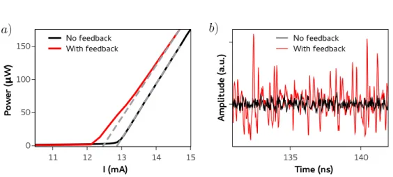
(24) 1.2. Semiconductor lasers with delayed optical feedback. 1.2.1. Optical characteristics of a semiconductor laser with and without feedback. In this section we illustrate the impact of optical feedback on the emission of a SL with an example. We use the laser described in Section 4.2. The light is reinjected into the laser using optical fiber components, as shown in the schematic in Figure 1.1. The loop is created by using an optical circulator, a three or four port device that routes incoming light from one port to another in a non-reciprocal way. A polarization controller and optical attenuator are included in the delay loop to control the feedback polarization and strength, respectively. The reinjected light can have different impacts depending on its properties, and even a tiny amount of the feedback can be enough to destabilize the SL [41, 42]. The polarization of the feedback light was set parallel to the polarization of the light emitted.. Semiconductor Laser. Polarization controller. Circulator. Optical attenuator. Figure 1.1: Schematic of an experimental setup in delayed feedback experiments using optical fiber components. The loop is created by connecting the third port of the circulator to the first port. The SL is connected to the second port. The black arrow represents the feedback propagation direction inside the loop, defined by the port connections’ of the circulator. Additional components can be included in the loop to control for the feedback’s properties. First, we characterize the output power emitted by the laser dependence to the bias current. This dependence is typically referred to as P-I curve. In Figure 1.2(a), the P-I curve shows the average power emitted by the laser versus the bias pumping current. In black, we show the PI curve of the SL in solitary conditions (without feedback), and in red with maximum available feedback. The curves are characterized fundamentally by the threshold current. This is the current where the laser 20.

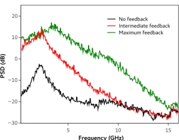
(25) Chapter 1. Introduction starts to emit stimulated light. This current is slightly larger than the current at which losses equal gain inside the laser, condition referred to as transparency [1]. For higher currents the output optical power increases linearly. For solitary conditions the threshold current is 12.87 mA. To obtain the threshold current, one can perform a linear regression analysis on the power emitted above threshold, which is represented as a gray dashed line in Figure 1.2(a). The crossing of the resulting linear fit with the x-axis at zero emitted power determines the threshold current. When optical feedback is injected, the curve shifts towards lower values. This is a well-known effect originating from a reduction of the total losses due to the re-injection of the emitted light into the laser [43]. This reduces the lasing threshold current and typically increases the output power emitted by the laser close to threshold. The feedback acts as an extra cavity and it changes the balance between the laser’s emission from the front to the rear facet. One can also observe that the slope of the dependencies are different. The solitary case presents a higher slope than under optical feedback, indicating a higher efficiency. The lower efficiency when including feedback is due to an effective increase of the reflectivity of the laser’s facet. Different slopes in the curves introduces a cross over point where the laser emits the same power with and without optical feedback present [22, 44]. Additionally, right after threshold, the P-I curve of the feedback laser experiences a kink before following a linear trend. This kink separates the P-I curve for the linear dependence shown as a gray dashed line in Figure 1.2(a). It was already observed in [43], where kinks are referred as irregularities. The power recorded for the P-I curves is the average power emitted in a time window much longer than the timescale of the laser’s dynamics. In Figure 1.2(b) we show the amplitude evolution of the dynamics with sub-nanosecond resolution. These traces were measured AC coupled, so the DC component of the signal is unknown. These traces were obtained for I = 13.25 mA. In black, we show the power over time by the solitary laser, and in red the laser with maximum available feedback. The laser with optical feedback presents larger and faster fluctuations than the laser under solitary conditions. The small fluctuations in the solitary case originate from experimental noise. To capture only the fast fluctuations on the power evolution we measure the power spectra of the dynamics as the power of the optical feedback increases, as shown in Figure 1.3. These power spectra were obtained by detecting the optical power evolution of the SL with a photodetector, and then measuring the spectra of the electrical signal with an Electrical Spectrum Analizer. In black, we show the power spectra on 21.

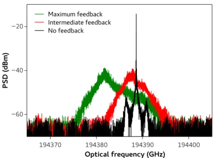
(26) 1.2. Semiconductor lasers with delayed optical feedback. No feedback With feedback. No feedback With feedback. Amplitude (a.u.). Power (μW). 150. 100. 50. 0 11. 12. 13. I (mA). 14. 15. 135. 140. Time (ns). Figure 1.2: (a) P-I curve and (b) example of power time series for the SL for solitary (black) and with optical feedback (red) for I = 13.25 mA. Gray dashed lines indicate extrapolations from linear regression analysis of the power versus current dependence. the laser under solitary conditions, in red for feedback attenuated by 12 dB, and green for maximum optical feedback. The power spectra of the solitary laser exhibits a pronounced peak at 2.5 GHz, corresponding to the frequency of the RO of the SL. When optical feedback is introduced, the emission spectra can substantially broaden. This indicates that the dynamic include faster and stronger oscillations as more optical feedback is added. The broad range of frequency components is a typical signature of chaotic dynamics. This relates to what we saw in the power time series, ruled by fast fluctuations of erratic amplitude. We finish by characterizing the spectra of the electrical field with an optical spectrum. In Figure 1.4 we show the optical spectra of the cases shown in Figure 1.3 with identical color. For solitary conditions, the spectra exhibits a sharp peak indicating a main emitted frequency with 10 MHz of linewidth (limited by the instrument). On the side, one can observe two small broad peaks corresponding to the damped RO. The amplitude of between these peaks is different due to the α factor. This asymmetry can be used to determine the α factor [45]. As feedback is injected, the spectra broaden. The dominant frequency emitted and the full spectra shifts to lower frequencies as more feedback is added. These effects can be explained by the Lang-Kobayashi model, which theoretically describes the SL under optical delayed feedback [46]. When including optical feedback, the model contains solutions called External Cavity Modes, responsible for the dynamical evolution [47–49]. In the phase22.

(27) Chapter 1. Introduction. 20. No feedback Intermediate feedback Maximum feedback. PSD (dB). 10. 0. −10. −20. −30 5. 10. 15. Frequency (GHz). Figure 1.3: Power spectra of the SL with different feedback conditions: no feedback (blak), 12 dB attenuated feedback (red), and maximum feedback (green). carrier density plane they are distributed in the shape of an ellipse, with an eccentricity determined by the value of α, and extending in the range p ω = κ (α2 + 1), where κ is the feedback strength [15, 17]. While solutions in the upper half of the ellipse are unstable, solutions in the lower side can be partially stable. The ellipse is tilted so the modes for negative frequency have higher gain, leading the dynamics towards those modes with high gain. Correspondingly, the emission shifts towards negative frequencies under optical feedback.. 23.

(28) 1.3. Semiconductor lasers under optical injection. PSD (dBm). −20. Maximum feedback Intermediate feedback No feedback. −40. −60. 194370. 194380. 194390. 194400. Optical frequency (GHz). Figure 1.4: Optical spectra of the SL with different feedback conditions: no feedback (black), intermediate feedback (red), and maximum feedback (green).. 1.3. Semiconductor lasers under optical injection. We have seen that the light emitted by the SL can be reinjected to stimulate complex dynamics. But light from another laser can also be injected. Optical injection is performed when the light from one laser (injection laser) is injected into another laser (response laser). This configures the lasers in a unidirectional coupling scheme. During optical injection, the injected light is meant to interact with the lasing directly, so the emission frequency of both lasers should be similar. For this reason, one can select and tune the source of the injected light so its has a frequency close to the one emitted naturally by the response laser. The idea of optical injection in lasers appeared shortly after the invention of the laser itself [50]. Optical injection in SL was triggered by the application of SL in optical communications [51]. It was demonstrated that the frequency and linewidth properties from the injection laser can be transferred to the response laser when the lasers are locked [52–54]. This is a coherent phenomenon where the response laser oscillation synchronize to the injection’s. Optical injection has been used to further stabilize lasers, ensuring 24.

(29) Chapter 1. Introduction single mode operation of the response laser to avoid multi-mode operation and mode hopping [55], reduce noise [56, 57], reduce linewidth [58], and to suppress feedback-induced instabilities. The emission of a single laser can be injected into multiple lasers to induce in all of them emission at the same frequency. Applications that require narrow linewidth can benefit from such scheme, like spectroscopy [59], laser cooling [60, 61], and traps for atoms [62]. Furthermore, optical injection can be also used in power amplifiers or for narrow optical filter. Optical injection can also induce nonlinear dynamics in the response laser. Under optical injection, nonlinear dynamics such as periodic oscillations, bistability, four-wave mixing, and chaos have been demonstrated [63–69]. The variety of nonlinear dynamics induced by optical injection in SLs makes these systems excellent testbeds for generation of complex dynamics. The generation of periodic oscillations can be employed for microwave generation [70]. Relaxation oscillations can be suppressed to increase modulation rates [71]. Additionally, optical injection can enhance the bandwidth of SL [72, 73]. The dynamics of SLs under optical injection have been extensively studied, theoretically [68] as well as experimentally [74]. Two parameters specially relevant for the dynamics of SL under optical injection are the injection strength and the frequency detuning. The frequency detuning is the optical frequency difference between the injection and response laser. If the frequency detuning is small and injection strong enough, the response laser is locked to injection and emits at the injection’s frequency. This dependence shows a cone in parameter space where the response laser is locked. Outside this region the laser is unlocked and nonlinear dynamics can occur [15]. The cone was derived for SLs for the first time in [75], and authors showed that α , 0 extended√the locking region asymmetrically for negative frequencies by a factor 1 + α2 . Linear stability analysis showed that locked solutions are stable on the most negative frequency side of the cone, while unstable elsewhere [15, 76]. Two SLs unidirectionally coupled is the simplest configuration to study optical injection in SLs. Instead of using a free-running SL one can use a SL with optical delayed feedback, either as the injection or the response system. This modification in the injection system can create a chaotic and broadband signal that the response laser needs to lock to. Incorporating the optical feedback into the response system, as the response laser can exhibit chaotic motion and can be forced to lock to injection even under the destabilization effect of the feedback. Incorporation of feedback in one of the two nonlinear elements has proved to enhance the complexity. 25.

(30) 1.4. Neuro-inspired information processing of the dynamics as well as broaden the bandwidth [77–80] , which has been useful for several applications [27, 81–86]. Some applications require information from injection with modulated signals. The dynamical response of a SL with optical feedback under such injection has been only very recently addressed [87]. Few studies have considered the injection of a chaotic signal from a similar system [79, 88] or even from the same one [89]. Nevertheless, typical modulation schemes like amplitude modulation involve holding a value over a specific time windows. This scheme differs to injecting a chaotic or a noisy signal. Deeper understanding of the properties of SLs under delayed optical feedback and modulated optical injection is required, especially to efficiently use them for information processing. This is the fundamental motivation in Chapter 4.. 1.4. Neuro-inspired information processing. In this section we move from nonlinear systems and focus on an information processing technique that benefits from complex dynamics. This technique is Reservoir Computing (RC). We make use of it in Chapter 4 and Chapter 5. Before describing in detail the intricacies of RC, we provide a brief background of the concept. RC belongs to the field of neural networks, a branch of Machine Learning. Neural networks has a biologically neuro-inspired origin. By mimicking the nervous system with an Artificial Neural Network (ANN), researchers desired to build a neuromorphic system that processes information with similar characteristics, functionalities as the brain. Fundamentally, the brain is a complex network of neurons, where every neuron is a nonlinear dynamical element connected to other neurons. The number of neurons in the brain varies among species, from 302 in simple worms as the C. elegans [90, 91] to 85 · 109 in humans [92]. The C. elegans shows around seven connections per neuron [91], while in the human brain the number of connections per neurons ranges from 150 to 1000 [93, 94]. Communication among neurons is performed via electrical current with a temporal distribution of spikes. ANNs do not attempt to replicate the brain. ANNs try to mimic the most basic structure of the brain, hence its name [95]. Up to now, implementations of ANNs do not reach the amount of neurons in a human brain, and they consider neurons with much simpler response functions. First implementations of ANNs were in the early 40’s [96]. The HodgkinHuxley model describes an excitable type of neuron, but neurons in ANN 26.

(31) Chapter 1. Introduction can operate with simpler nonlinear dynamics. Now there are many neuronal models more or less complex [97]. One of the most basic ANN models are the Feed-forward Neural Networks (FNNs). In FNNs, the neurons are arranged in layers and all the connections are from one layer to the next one (i.e. feed-forwarded). In Figure 1.5 we depict a FNN consisting of neurons arranged in three layers. Layers are the input layer, the hidden layer, and the output layer. Neurons are connected all to all from one layer to the next. Every connection has a connection strength called weight, which determines how much the output of a neuron affects another. Connections that run from the input to the hidden layer and from a hidden layer to the output layer are called input weights and output weights, respectively. FNNs can have multiple hidden layers and the number of neurons in each layer depends on the task at hand.. Hidden Layer Input Layer. Output Layer. Figure 1.5: Example of an ANN. Triangles represent nodes in the input layer, circles represent nodes in the hidden layer, and squares represent nodes in the output layer. Dashed arrows represent input weights, while the dotted arrows output weights. A fundamental neuron applies a nonlinear transformation, typically referred to as activation function, to the weighted summation of input signals from other neurons as shown in Equation (1.2). ! x lj+1 = f NL. ∑ ωlj,i · xil , θ. (1.2). i. 27.

(32) 1.4. Neuro-inspired information processing Here f NL is the activation function, xil is the output of the neuron i in the layer l, ω lj,i is the weights from the neuron i in layer l to the neuron j in layer l + 1, and θ are other internal parameters. Different activation functions can be used, but the most employed are the rectified linear unit (ReLU) and sigmoid functions (e.g. hyperbolic tangents) [98–100]. Still, simplified models of neurons dynamics like the Integrate-and-Fire can be used, which are more realistic than sigmoid functions but carry much more computational costs [101]. The input layer is the one that introduces information into the system as stimulus for the dynamical system. Information flows through the hidden layer depending on the weight arrangement and parameters. The state of the output layer encodes the output of the system to the injected information, and can be calculated from the state of the last hidden layer as in Equation (1.3). 0. out yk (n) = ∑ ωk,i · xil (n). (1.3). i. Here xil is the output of the neuron i in the last hidden layer l = l 0 , yk is out is the weight from the the state of the node k in the output layer, and ωk,i neuron i in the last hidden layer to the neuron k in the output layer. ANNs promised important advances in sensor control and processing as well as in tasks where the brain excels such as pattern (e.g. speech and image) recognition or decision-making. The vast configuration possibilities allows these systems to implement a broad variety of different nonlinear transformations of the input data according to the required task. But to make ANNs successful, it is necessary to find an optimal configuration of weights of the connections, number of layers, and number of nodes in each layer. An optimal configuration is one that minimizes the errors made by the ANN in a specific task. Finding such configuration is called learning, where the ANN is trained. Calculating the output of the network is simple but training can exhaust computational resources. As the number of weights in the system increases faster than the number of nodes, and weights are typically real numbers, the amount of configurations increases substantially. Due to the computing requirements, the first simulations of an ANN would not be conducted until 1955 at the IBM Research Laboratories [102]. The first experimental implementation was realized in 1959 with a circuit called (M)ADALINE, that was successfully implemented for adaptive removal of echoes in telephone lines [103]. (M)ADALINE included memistors, an early 3-terminal implementation of memristors made from an electroplating cell. The first successful multi-layer network was presented few years later, in 1965 [104]. Illusions 28.

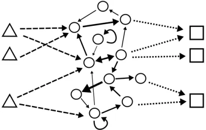
(33) Chapter 1. Introduction in the field greatly vanished in 1969 after [105] showed that perceptrons, a type of basic neural network, could not process the XOR circuit, and that the computational resources to handle large neural networks were too high to the computers at that time. New interest re-emerged when in 1974 the back-propagation algorithm was published, which allowed the weights of FNNs to be trained efficiently [106]. While ANN with more nodes, layers, and efficient learning algorithms were developed, a new kind of neural networks with a different connectivity was invented [107]. These new ANNs, called Recurrent Neural Networks (RNNs) introduced recurrent connectivity among the neurons in the network. In RNNs there is not only connectivity among nodes in the hidden layers, but also cyclic connections and self-connections, which allowed the response of a neuron to return to the same one after passing through other neurons. An example of a RNN is shown in Figure 1.6. In FNNs, perturbations inside the network travel only forward towards the output layer. Recurrence allows for the appearance of temporal dynamics in the network. In the RNNs the information resides in the network, encoded in its dynamical state, creating an internal memory. Therefore, previous inputs could be extracted time after they were injected and could be used for subsequent computation together with more recent inputs. On the contrary, FNNs are memoryless and their present output only depend on the current input. The idea of introducing recurrence in ANNs was popularized in [108], while [109] suggested that the brain could have this kind of connectivity to account for memory. Besides the biological plausibility of recurrence in neuronal systems [95, 110], recurrence in ANNs was an important milestone since many tasks require memory. It has been shown that RNN can be Turing equivalent, i.e. capable of solving any recursive function [111]. RNN exhibits excellent performance even nowadays in combination with other techniques in tasks such as speech recognition [112], translation [113], image caption [114], and prediction [115, 116].. 29.

(34) 1.4. Neuro-inspired information processing. Figure 1.6: Example of a RNN. The hidden layer is a recurrent network. Connections between nodes are represented by solid arrows, with thickness representing the different connection weights.. 1.4.1. Reservoir computing. While powerful, RNN are difficult to train. The training methods used for FNNs could not be applied due to the recursiveness of the network. The training algorithms available for RNNs were too slow [117, 118]. In the early 2000’s, several independent works helped to solve this problem by demonstrating that successful performance in RNNs could be obtained by only training the output weights. They called this approach Echo State Network (ESN) [119], Liquid State Machine [120], and Back-Propagation Decorrelation [121]. In this framework, the hidden nodes create a recurrent network called the reservoir. Eventually, these methods were unified under the common name of Reservoir Computing (RC) [122, 123]. By reducing the number of weights that are modified, the RNN learning is much simpler and reduce its costs. The computational power of reservoir computers arises from their capability to map the injected information onto a high dimensional space. Reservoirs are typically made of hundreds or thousands of nodes to ensure that the reservoir provides a space with enough dimensionality, since a higher dimension increases the chance of successful performance [124]. Information that is injected through the input layer has a certain dimensionality, such that inputs are not linearly separated. The reservoir creates a state space with higher dimensionality than the input space. The nonlinear mapping of the inputs in this higher dimensional space arranges 30.

(35) Chapter 1. Introduction them in a new way, such that they become linearly separable. In classification tasks, for example, this means that the inputs that are not separated in their original phase space can be now separated by hyperplanes in the reservoir’s state space, where the output weights are their defining parameters. To successfully operate, the reservoir computer needs to fulfill certain properties [123, 125, 126]: the separation property, approximation property, consistency, and fading memory. The separation property refers to the ability of the reservoir to provide sufficiently different responses to inputs that belong to different classes. This property allows for inputs to be more easily separable once they are mapped in the high dimensional space of the reservoir. Nevertheless, the responses of the reservoir need to be resilient to small changes in the inputs, since similar inputs of the same class need to be classified identically and not create diverging different responses in the reservoir. This corresponds to the approximation property [120]. Consistency refers to the ability of the reservoir computer to provide similar responses to the injection of similar input, hence robustness to potential noise in the input and the system itself. If the reservoir responses would not be consistent, the high dimensional projection would not be the same for identical input, and the output weights could not be efficiently optimized. And last, fading memory means that the memory in the system needs to disappear after some time. This means that the dynamical response of the reservoir to an input is affected by the recently injected inputs, but not by the once injected long time ago.. 1.4.2. Delay-based reservoirs. The typical RC is a recurrent network of multiple nodes randomly connected (as in Figure 1.6). However, deterministic network topologies can be successfully used [127, 128]. A viable RNN topology is a circular network of unidirectional coupled nodes, as the Simple Cycle Reservoir in [127]. This topology is of particular interest because it can be implemented via a single nonlinear node under the influence of delayed feedback [129]. This approach is called Time Delay Reservoir (TDR) [130]. The typical TDR is illustrated in Figure 1.7. TDR makes use of the high dimensionality of delay systems to create the state space required for RC. Delay systems are specially suited for this task as the state space is infinite dimensional. This occurs since their state at time t depends on the state of the system in the time interval, defining τ as the delay time, [t − τ, t). In theory this creates an infinite dimensional system. However, in practice the dynamics of delay systems are not infinite dimensional due to finite 31.

(36) 1.4. Neuro-inspired information processing dynamical bandwidth [131]. In TDRs, the temporal evolution of the nonlinear element determines the state of the nodes in the network. More exactly, the state of an individual node is obtained by interpreting the response of the nonlinear element over a time interval equal to θ. The network is then the collection of consecutive nodes responses during a time interval τ. Since the θ intervals of different nodes do not overlap, the number of nodes in the reservoir N is defined by N = τ/θ. The network connectivity in a TDR originates from two contributions. One of these is the feedback connectivity. Since τ is a multiple of θ, every node receives from the feedback its state in the previous τ interval. The strength of this connectivity is related to the feedback strength. Therefore, the feedback strength strongly influences the nonlinear dynamics exhibited by the reservoir and their memory. The other connectivity is from a node to the following ones in the unidirectional network [129]. The dynamical response of a node can influence the response of subsequent nodes due to the inertia in the dynamics, which can be controlled by adjusting the parameter θ (and the characteristic time scale of the dynamics if possible). If θ is smaller than the characteristic time scale of the nonlinear element, then the response of the nodes will affect multiple nodes down the network. On the other hand, if θ is larger than the response time of the characteristic node, then the connectivity among nodes is reduced and nodes behave as if they were isolated. An extremely small θ is also not desired, since such short time interval would not allow time for the nonlinear element to develop a response to the information being injected. Other configurations use a network with a duration different than the delay time to exploit different connectivities [132]. Therefore, the selection of the interval time θ is crucial. A θ = 0.2 · T, where T is the characteristic time of the nonlinear node dynamics’, is a typical value employed in literature. Once the state of the reservoir is known, an output layer as the one described in Equation (1.3) can be used to obtain the output of the RC.. 32.

(37) Chapter 1. Introduction Reservoir. Input weights (ωinput). Output weights (ωoutput). Temporal mask. NL Θ. Figure 1.7: Illustration of the TDR. The reservoir is now a circular network of nodes, separated homogeneously over the delay time. This case shows the input and the output layer with just one nonlinear element. Not only the dynamics of the reservoir are essential, how information is injected plays an important role. In a TDR the nodes are multiplexed in time, so the input layer requires a methodology illustrated in Figure 1.8. Every input of information to be processed is typically injected to all the nodes in the network by time multiplexing. This means injecting the value into the nonlinear element over a time interval τ, as shown in Figure 1.8(a). But by doing so, the response of the nonlinear element would relax to a stationary state (if operated from a stable fixed point) since the relaxation time is much shorter than the delay time. This scenario would correspond to having many nodes of the TDR with identical responses. To keep the reservoir generating different transient dynamics, every input data is multiplied with a function called the mask. This mask is a stepwise function and has a number of values equal to the number of nodes. In Figure 1.8(b) we show an example of a mask with only five values for illustrative purposes. In Figure 1.8(c) we show the resulting injected signal for the reservoir. Every mask value is associated to an individual node in the reservoir. Therefore, the mask values strongly determine the input weights in the reservoir. Not every configuration of input weights is adequate for computation. The input weights need to create responses in the reservoir with sufficient diversity. This process benefits performance of the reservoir computer since it enriches the nonlinear mapping. 33.

(38) 1.4. Neuro-inspired information processing If sequences of weights are repeated, nodes will exhibit similar responses and the diversity of the reservoir state decreases. Therefore, a mask with high variation of values is desired. Design of optimal input masks have attracted interest due to their clear impact on the performance of these reservoirs, and several proposals have been presented [87, 133]. Nevertheless, TDRs present an important difference. The multiplexing of the nodes in time slows the system compared to spatial networks by a factor equal to the number of nodes. Real time processing can be affected then by this feature. The ability to create an entire network of interconnected nodes, all of them with nonlinear dynamics, with just a single element attracted a lot of interest. While other systems required many individual components and the capacity to connect them (spatially distributed networks), TDRs do the job successfully with fewer components. Mask. Reservoir input. Input data. θ. 𝜏 Figure 1.8: Illustration of the masking process. Each value of the data input sequence (a) to be processed is multiplied by the mask (b), resulting in the signal that is finally injected into the TDR (c).. 1.4.3. Hardware implementation. Nowadays, ANNs have proved to be a state-of-the-art technique for a broad variety of applications including decision-making [134, 135], navigation [136–138], robot control [139], pattern recognition and processing [140, 141], and even drug design [142]. This was driven fundamentally by the exponential increase of computational power (that provided the power to train the networks in a tolerable time) and of raw data (necessary to train the networks with sufficient examples). In spite of their 34.

(39) Chapter 1. Introduction successful performance, ANNs still have a high computationally cost. In contrast, a human brain works very efficiently with little power. Therefore, there is room to explore hardware implementations of ANNs (devices with nonlinear elements connected as a network) that offer better possibilities with better efficiencies than its transistor-based computers. For this purpose, many efforts have been made to develop information processing devices that mimic neural systems. Individual neurons have been emulated with traditional circuit elements [143, 144]. Hardware implementations have explored multiple mediums and nonlinear elements, including: electronic circuits with spiking silicon neurons [145–147], spintronic oscillators [148], tensegrity robotic structures [149], and liquids [150]. Real biological neurons have even been used to harness computational power with RC [151]. But interestingly, hardware implementations of ANNs can be done with optical systems. Optical implementations of neuromorphic computers using TDRs are very desirable. Optical systems could provide benefits like high processing speed for even real time processing thanks to the fast speeds of photonic devices. Optical systems could provide the large connectivity that ANNs requires in a small space and broadcasting from one node to many others. Several approaches have been explored to connect the optical nodes and control their weights [152–155]. Implementation of the nonlinear nodes can also be done with a varierty of optical devices. Thin films optical amplifiers and optical bistability were recognized as candidates for nonlinear operation [156]. Excitable photonic devices have also been studied for its application in neuromorphic computing, including devices like microdisk lasers [157], graphene-based excitable laser [158], and saturable absorber laser [159]. Many nonlinear optical elements have proved ANN computing capabilities including Semiconductor Optical Amplifiers (SOAs) [132, 160, 161], photodetectors [152, 162, 163], ring resonators [164], SLs [29, 165], and modulators [166, 167]. Photorefracive crystals are also components that provide tunable weights and nonlinearity suitable for ANNs [168–170]. All these systems have proved capabilities for information processing with ANN techniques, with new implementations and concepts appearing for better and larger implementations, demonstrating the strong interest, possibilities, and future of the optical computing with ANNs.. 35.

(40) 1.5. Motivation and overview of this thesis. 1.5. Motivation and overview of this thesis. In this chapter we have introduced the SL and the complex dynamics that can arise under the influence of optical perturbations. SLs are capable of exhibiting a rich complex behavior, which is used to study these dynamics experimentally in a fundamental level. Furthermore, complex dynamics have been put to use in multiple applications, encouraging the understanding of such behaviors. For these reasons, in this thesis we aim to further study the dynamics of delayed photonic systems, use the complex dynamics of the SLs in information processing applications, and design and implement new nonlinear optical systems for application as reservoir computer. The thesis is organized as follows. In Chapter 2 we describe the methodologies used for our experimental realizations. This includes how optical power and optical spectra have been measured and what techniques we used to determine the optical delay. In Chapter 3 we study the impact of using more than one optical delay feedback in the dynamics of a SL. Delay systems have been used to study the dynamics of systems with one spatial dimension [171, 172]. The implementation of multiple delays could be used to extend the analogy to study systems with more spatial dimension. We will use a SL under delayed optical feedback due to their well-known rich dynamics under delayed feedback, and include an additional optical delay line orders of magnitude longer than the first one. This will induce new dynamical states, and we will study its features and similarities to other nonlinear systems. Chapter 4 studies the use of a SL under optical feedback and modulated optical injection as a TDR in an optical reservoir computer. The nonlinear dynamics present in a SL under the simultaneous influence of optical feedback and injection are centered for this information processing application. The impact of optical injection that is modulated in such systems has not been studied in detail, we will also evaluate how the modulation affects the dynamics of the system. In this chapter we will evaluate the impact of key parameters on the performance and properties of the system. The last chapter, Chapter 5, develops an optical reservoir computer by building a large spatially extended network of nonlinear optical elements. This reservoir implements hundreds of nonlinear nodes with few components, and couple them simultaneously using passive components. We will also implement experimentally the output layer in hardware, introduce learning rules, and demonstrate successful operation with low 36.

(41) Chapter 1. Introduction errors in a task despite current experimental limitations. The final chapter of the thesis will be the final conclusions of this research, and a collection of future prospects.. 37.

(42) 1.5. Motivation and overview of this thesis. 38.

(43) Chapter 2. General methods. 39.

(44) 2.1. Light measurement acquisition methods. 2.1. Light measurement acquisition methods. Different characteristics of the light can be measured with different instruments. Here we describe the instruments employed to measured them in this thesis. Average optical power The average optical power of the light was measured using a Thorlabs power meter console with a power sensor. The sensor converts the optical power into a voltage. The console reads the voltage from the sensor and provides a power measurement taking into account the responsiveness of the sensor to the selected wavelength on the console. These devices provide optical power measurements of slow changing fields due to their bandwidth of 100 KHz, which we refer to as the average optical power. For experiments where the light’s wavelength was around 1550 nm (Chapter 3 and Chapter 4) we used a PM100D console and a S154C sensor. This sensor is a InGaAs photodiode with a high responsivity in the 1550 nm, and a power range between 100 pW and 3 mW with 10 pW resolution. For experiments where the light’s wavelength was around 660 nm (Chapter 5) we used a PM100A console and a S150C sensor. This sensor is a Si photodiode with adequate responsivity at 660 nm, and a power range between 100 pW and 5 mW with 10 pW resolution. Time evolution of the optical power Measurements of the temporal evolution of the optical power at fast timescales are crucial to observe the dynamics of an optical system. The dynamics of a SL can appear with speeds ranging from MHz to GHz, so fast detectors and acquisition systems are required. For these conditions, we used a fast photodetector to convert the optical signal into an electrical one and an oscilloscope to acquired the electrical signal. The photodetector used was a MITEQ SCMR − 100k20G − 30 − 15 − 10 − FA. This photodetector works in the wavelength range from 1280 to 1580 nm, and offers a bandwidth from 100 KHz to 20 GHz. As an oscilloscope we used a Teledyne Lecroy oscilloscope, model Wavemaster 816Zi. This oscilloscope has a sampling rate of 40 GSa/s, so with a time resolution of 25 ps, and an analog bandwidth of 16 GHz. The oscilloscope’s bandwidth limited the fastest dynamics that could be recorded to 16 GHz, enough to observe the fast dynamics of SL systems.. 40.

(45) Chapter 2. General methods To improve the Signal-to-Noise ratio (SNR) of the recorded signals we added before the photodetector a SOA and a Optical Tunable Filter (OTF), as shown in Figure 2.1. The SOA is a polarization insensitive optical amplifier, similar to a SL but without the resonator cavity. This one is a Covega 1013XS, wavelength centered at 1550 nm. Amplification of the signal reduces the negative effects of noise in the photodetector and in the oscilloscope, enlarging the small features in the signal against the noise in the photodetector. To improve the benefits of the SOA we use it together with an OTF. The SOA emits spontaneous emission in a broad frequency spectrum that acts as noise added to the amplified signal. The OTF is a tunable bandpass filter, that once applied to the amplified signal removes the spontaneous frequency components outside the frequency range of interest. Our OTF is a Santec OTF-350, with a passband flat-top filter shape and isolation above 50 dB.. SOA. OTF. Fast Photodetector. Oscilloscope. Figure 2.1: Detection section of the setup. Components used to detect the temporal evolution of optical signals and improve its SNR. Blue lines are optical fibers, orange lines are electrical cables. Power spectra The power spectra provides the amplitude of the different frequency components of the intensity field of the light, and we measured it with an Anritsu MS2667C. It is measured with an ESA from the electrical signal generated from the photodiode upon receiving the optical signal. This device measures the frequency spectra from 9 kHz up to 30 GHz. In practice the bandwidth is limited to 16 GHz due to the bandwidth of the electrical cables carrying the signals. Optical spectra To measure the optical spectra of the optical signal we employed two different Optical Spectrum Analyzer (OSA) depending on the require41.

(46) 2.2. Experimental techniques for precise determination of the delay time ments. One instrument was an Anritsu MS9710C, an OSA based on a diffraction grating which provides a wavelength resolution of 0.1 nm in the 600 to 1750 nm range. It also offers 70 dB dynamic range with 0.1 dB resolution and −90 dBm optical reception sensitivity. This high sensitivity allows to even resolve the non-emitting longitudinal modes in SLs. The second OSA is a high resolution one from Aragón Photonics, model BOSA 210. The ”B” stands for Brillouin, as the analyzer combines the high power of a tunable laser source with the signal under test to stimulate the nonlinear Brilloun scattering on an optical fiber to create a narrow filter. This operation principle provides the BOSA with an 10 MHz resolution from 1530 to 1565 nm, capable of for example highly resolving the spectra of SL exhibiting complex dynamics.. 2.2. Experimental techniques for precise determination of the delay time. Precise determination of the delay time is important in the study of delayed systems [173–176] and in the research of following chapters, since in Chapter 3 and Chapter 4 require delay times to be precise multiples of other quantities. To ensure these requirements are satisfied as close as possible we make use of the techniques described in the following.. 2.2.1. Autocorrelation measurement of timetraces. The delay time can be extracted from the temporal evolution of the dynamics by evaluating its Autocorrelation Function (ACF). This method has been used previously in SL under optical delayed feedback in the context of chaos-based communications [176]. The ACF is defined in Equation (2.1). ACF (t0 ) =. h( x (t) − h x (t)i) ( x (t + t0 ) − h x (t)i)i σx2. (2.1). where x (t) is the time evolution, hi denotes time average, and σx = h( x (t) − h x (t)i)i1/2 . The ACF shows how similar are the values of x (t) separated by t = t0 when averaged over all the timetrace. To extract the time delay from the intensity dynamics of a SL with delay feedback, the autocorrelation function needs to present periodic sharp peaks. The main peak would observed at t0 = 0, while the first peak is found for t0 corresponding to the delay time. The time delay of the system can be extracted 42.