Does Aid Promote Donor Exports? Commercial Interest versus Instrumental Philanthropy

Texto completo

(1) . . Título artículo / Títol article:. Does Aid Promote Donor Exports? Commercial Interest versus Instrumental Philanthropy. Autores / Autors. Martínez Zarzoso, Inmaculada; Nowak Lehmann, Felicitas; Parra Robles, María Dolores; Klasen, Stephan. Revista:. Kyklos, 2014, vol. 67, no 4,. Versión / Versió:. Pre-print. Cita bibliográfica / Cita bibliogràfica (ISO 690):. url Repositori UJI: . MARTÍNEZ‐ZARZOSO, Inmaculada, et al. Does Aid Promote Donor Exports? Commercial Interest versus Instrumental Philanthropy. Kyklos, 2014, vol. 67, no 4, p. 559-587. http://hdl.handle.net/10234/126578.

(2) Does aid promote donor exports? Commercial interest versus instrumental philanthropy (03.07.2015 ) forthcoming in Kyklos AUTHORS: Inmaculada Martínez-Zarzoso (corresponding author) Department of Economics and Ibero-America Institute for Economic Research, University of Göttingen and Institute of International Economics, Universidad Jaume I (Spain). Platz der Göttinger Sieben 3; 37073 Göttingen; Germany; Ph.: +49 551 399770; Fax: +49 551 398173; e-mail: [email protected] Felicitas Nowak-Lehmann D. Ibero-America Institute for Economic Research and Center for European, Governance and Economic Development Research at the University of Göttingen e-mail: [email protected] M. D. Parra, Department of Economics, Universidad Jaume I (Spain). E-mail: [email protected] Stephan Klasen Department of Economics and Courant Research Centre on Poverty, Equity and Growth in Developing and Transition Countries, University of Göttingen e-mail: [email protected]. 1.

(3) Does aid promote donor exports? Commercial interest versus instrumental philanthropy Abstract This paper investigates by means of advanced panel data techniques whether bilateral aid has been successful in promoting bilateral exports to recipient countries during the period 19882007 and to what extent changes in aid policies have influenced this relationship. The main novelty of this research is the distinction between tied and untied aid in a multi-donor gravity model of trade and the comparison between trade and aid policies in this setting. We find an average positive effect of bilateral aid on exports, which varies over time and across donors and which appears to depend on the extent to which donors tied aid to exports. The effect does appear to have decreased substantially over the period studied and it is even not statistically significant in the 2000s, which could suggest that the recommendations given by the OECD Development Assistance Committee (DAC) concerning the untying of aid and aid allocation have been followed by the donors and led to declining impacts on their exports. Interestingly, these decreasing aid-elasticities are accompanied by increasing coefficients of the regional trade agreement variable, which is positive and statistically significant after 1994. Finally, we find that the strength of the relationship between exports and bilateral aid is correlated with the extent to which aid is tied and partially related to the sectoral allocation of aid. Key words: exports, foreign aid, donors, panel data, gravity model, tied aid JEL Classification: F10; F35; O10 1. Introduction In recent decades, some research effort has been devoted to investigating the effects of developmental assistance on the economic performance of the recipient countries and on clarifying how aid can be used to promote exports from developing countries, the so-called “aid for trade” principle (Morrissey, 2006; Portugal-Perez and Wilson, 2009; NowakLehmann D., Martínez-Zarzoso, Klasen, Herzer and Cardoso, 2013; Calí and Te Velde, 2011). Much less attention has been devoted to the issue of quantifying the impact of aid on donors’ export revenues (Suwa-Eisenmann and Verdier, 2008). The literature on aid allocation has found that aid flows depend strongly upon historical ties and strategic and economic interests, and less strongly dependent upon poverty levels or the existence of democratic governance in recipient countries (Alesina and Dollar, 2.

(4) 2000; Doucouliagos, H. and Paldam, 2006). Hence, an interesting question is to what extent commercial interests of the donor are indeed promoted by the aid relationship. There might also be a reverse causal relationship from commercial relations to aid flows. Younas (2008) finds that a larger amount of aid is provided to recipients who import capital goods and Martínez-Zarzoso, Nowak-Lehmann D. and Johannsen (2012) show that aid increases with donor’s exports. This evidence partially supports the trade benefits motive for giving aid. Indeed, donors’ aid policies could then be compared to other trade promotion policies such as regular trade missions and state visits (Rose, 2007; Head and Ries, 2010) or to the formation of regional trade agreements (RTAs). Surprisingly, the related empirical evidence on whether aid promotes donors’ trade interests is still limited. A number of studies focused on the effect of aid on export levels for a given donor (Zarin-Nejadan, Monteiro and Noormamode, 2008; Nowak-Lehmann D., Martínez-Zarzoso, Klasen and Herzer, 2009; Martínez-Zarzoso, Nowak-Lehmann D., Klasen and Larch, 2009). A few others have analyzed the effect of aid on donor countries’ export levels from a multi-donor perspective (Nilsson, 1997; Lloyd, McGillivray, Morrissey, and Osei, 2000; Wagner, 2003; Nelson and Juhasz Silva, 2012; Johansson and Pettersson, 2013), all of which leave open some methodological and/or substantive questions. For instance, these multi-donor studies failed to incorporate the so-called multilateral resistance factors into the gravity model of trade (Nilsson, 1997; Wagner, 2003; Nelson and Juhasz Silva, 2012) and to control for unobserved heterogeneity (e.g. Johansson and Pettersson, 2013), or focused only on a few donors (Lloyd, McGillivray, Morrissey, and Osei, 2000). We mainly depart from the existing literature by distinguishing between tied and untied aid in the multi-donor gravity model of trade and by using novel panel-data techniques that overcome the above-mentioned methodological issues. None of the above-mentioned papers incorporated data on tied aid in their models and most of them fail to properly control for heterogeneity issues. More specifically, our own analysis contributes to the multi-donor perspective studies in two fronts. Firstly, we extend the existing empirical literature by paying special attention to donors’ heterogeneity, using more recent data, additional covariates (other donors’ aid, exchange rates and RTAs), and more advanced econometric techniques, which enable us to incorporate multilateral resistance factors and unobserved heterogeneity into the analysis. In particular, we depart from previous multi-donor studies such as Nilsson (1997), Wagner (2003), Nelson and Juhasz Silva (2012) and Johansson and Pettersson (2013) in the way we control for unobserved heterogeneity (we use dyadic fixed effects) and multilateral resistance factors (country-and time fixed effects). Secondly, from a policy point of view our 3.

(5) contribution is to address the following key questions. First, we ask to what extent donor countries benefit from bilateral and multilateral development aid in a multi-donor-multirecipient set-up and in terms of greater donor exports to the recipient countries and to what extent this depends on specific aid policies. It is worth noticing that we are the first authors to investigate in a multi-donor framework whether the tying status of each country is able to explain the different aid effects on donor exports. Second, we investigate to what extent a given bilateral commercial link, a donor-recipient link, displaces other donors’ exports, generating a crowding-out effect. To our knowledge this issue has only been investigated for Germany and the Netherlands. Finally, this is the first paper that investigates whether there has been a change in the trade-aid relationship as a consequence of the international recommendations (e.g. by the Development Assistance Committee of the OECD, DAC) on untying official development assistance. To summarize our main results, we find that the increase in the amount of donors’ exports flowing from donors’ aid is more moderate than in earlier studies: around $0.50 for every aid dollar spent in the short run, rising to up to $1.8 US increase in exports for every aid dollar spent in the long run. The overall effect is remarkably robust, but decreases over time for most donors. In particular, from 2000 onwards a lower (and even insignificant) effect of bilateral aid on the corresponding donors’ exports is found. Since the late 1990s donors have increasingly been signing RTAs with developing countries as an alternative way to promote their commercial interest. We do not find evidence of a displacement effect for all donors, but only for European Union donors. Interestingly, the evidence indicates that aid from some donors is not export-enhancing, whereas for some others, the effect is strong and robust to several specifications. The effect is remarkably high for some donors (Austria, Australia, Italy, Japan, Sweden, US, Germany, Canada and Spain) and positive but smaller for France, UK, Norway, Denmark and Portugal. However for others, we find no such effect (Belgium, Finland, Greece, Ireland, Netherlands1, New Zealand, and Switzerland). We find suggestive evidence that this could be due to the tying status of aid as well the different sectoral allocation among donors. Donors for which aid promotes trade are characterized for having higher levels of tied aid (France, Austria, Australia, Canada, Spain) or for giving aid for specific purposes (e.g. The Norwegian Oil for Development (OfD) initiative2). On the 1. In Martinez-Zarzoso et al. (2014) we examine this question for the Netherlands only, considering a longer time period. We find that, overall, there has been a positive effect of Dutch aid on Dutch exports to recipient countries but that this effect has oscillated over time. The time period included in this paper is the one which had the lowest effect of aid on exports. In this sense the results are not inconsistent with each other.. 2. http://www.norad.no/en/Thematic+areas/Energy/Oil+for+Development. 4.

(6) other hand, countries in the second group are characterized for having lower levels of tied aid (Ireland, Netherland, Finland) or for giving aid mainly for social infrastructure and services (New Zealand, Greece and Belgium), where the export effects are apparently lower3. Section 2 summarizes the related literature and sets up the theoretical framework. Section 3 presents a description of the data. Section 4 presents the model specification, discusses the main results, and presents a number of robustness checks. Finally, Section 5 outlines some conclusions. 2. Theoretical Framework and Literature Review Early literature on the welfare effects of bilateral transfers between countries raised the possibility of transfer paradoxes (e.g. Leontieff, 1936). Applied to aid the paradox means that foreign aid can be donor-enriching and recipient-immiserizing due to terms-of-trade effects associated with the aid flows. Since those preliminary discussions, the theoretical literature on transfer paradoxes has been extended to more general settings (Gale, 1974; Brecher and Bhagwati, 1981 and 1982; Bhagwati, Brecher, and Hatta, 1983 and 1984). The findings indicate that the paradoxes are still possible but, under certain conditions both donors and recipients can benefit from transfers (weak paradox). In this line, Djajic, Lahiri, and Raimondos-Moller (2004) studied the welfare implications of temporary foreign aid in the context of an intertemporal model of trade and considered the impact of aid on donor and recipient exports. The authors found that in the presence of habit-formation effects, aid may serve to shift preferences of the recipient in favour of the donor’s export goods in future periods. As a consequence, the intertemporal welfare gain of the donor is positive under certain conditions, namely when the terms-of-trade effect associated with this shift is sufficiently large and the real rate of interest is sufficiently low. Taking the gravity model of trade as a theoretical framework, Nelson and Juhasz Silva (2012) present an extension of Anderson and van Wincoop (2003) to modeling trade flows to the asymmetric north-south case and derive some implications related to the effect of aid on trade. Their results indicate that if the economy of a donor country (GDP) is larger than that of the recipient country by at least the monetary value of the foreign aid, there is an increase in exports from the larger country to the smaller. The intuitive rationale behind this effect is that, as a result of the transfer, the two countries become more similar in size, and the more similar in size two countries are, the more they trade with one another.. 3. At the same time, one should treat these country-specific effects and their interpretation as suggestive as the effects might differ over time and we consider a particular time window here. 5.

(7) Turning directly to the empirical literature that investigates the impact of aid on a donor country’s exports, we classify the studies according to the underlying mechanism that generates the aid-trade relationship. Four mechanisms are identified in the related literature: First, aid could have a trade promoting effect and can act as a “door opener” for a given bilateral relationship (donor-recipient). Closely related to this, aid can have an effect on overall bilateral trade, promoting also exports from recipients to donors.4 Third, the bilateral link can generate a good-will or familiarity effect that also promotes donor’s exports. Finally the bilateral link could also give rise to a displacement effect decreasing exports from other donors to a given recipient. Concerning the trade promoting effect of development aid, in the 1990s some authors emphasized that it is critical to distinguish between the effects of tied and untied aid. In particular, Jepma (1991), Arvin and Baum (1997) and Arvin and Choudry (1997) evaluated the relationship between bilateral aid and bilateral exports with and without tying of the aid and found that aid without tying was roughly as export-promoting as tied aid. The authors pointed out that the reasons could be the existence of parallel trade agreements and trade concessions or the effects of the recipient countries’ good will5. However, these authors focused on a limited number of donors and used modeling strategies that depart from the gravity model. In addition, their data were only until 1990. In more recent years tying has been progressively reduced, partly due to pressure from the DAC. The second mechanism has been scarcely investigated, to our knowledge only Johansson and Pettersson (2013) and Nowak-Lehman D. et al (2013) investigate the effect of bilateral aid on recipient exports. While the first study finds a positive and significant effect of aid on recipient exports, the second study finds that the long-term impact of bilateral aid on recipient exports is not statistically significant after controlling for bilateral (dyadic) fixed effects, autocorrelation and endogeneity. The reason could be that Johansson and Pettersson (2013) failed to control for unobservable heterogeneity related to each bilateral relationship (dyadic fixed effects); to the extent that these fixed effects used in Nowak-Lehmann et al. (2013) capture time-invariant goodwill that affects both the trade and the aid relationship, aid might be a way to promote this goodwill and therefore should augment trade flows in both directions. Related to this, a third group of studies pointed towards a good-will or familiarity effect as the main underlying mechanism explaining the relationship. Aid may facilitate trade by creating new customers relations, building reputation or opening distribution channels. 4 5. This issue is examined in detail by Nowak-Lehmann, Martínez-Zarzoso, Herzer, Klasen and Cardoso (2013). Recent evidence shows that less tying does in fact lead to less exports (Johansson and Pettersson, 2013). 6.

(8) Nilsson (1997) investigated the aid and trade relationship of EU countries and developing countries from 1975 to 1992 using three-year averages and showed that $1.00 US-worth of aid increased exports by an average of $2.60 US for EU countries. He also failed to control for unobservable heterogeneity since he used a common intercept for all countries and a time trend. In a similar framework, Wagner (2003) studied the aid and trade relationship between OECD donors (especially Japan) and recipient countries. Using pooled OLS for the years 1970, 1975, 1980, 1985, and 1990 he computed the donor-country export-level impact of $1.00 US of aid to be approximately a $2.30 US return, however, when fixed country effects were added it was reduced to $0.73 US return. Nelson and Juhasz Silva (2012) also found an average positive effect of foreign aid on exports from the donor to the recipient, but failed to account for dynamics and multilateral resistance effects. Similarly, Nowak-Lehmann D. et al. (2009) and Martínez-Zarzoso et al. (2009) focused in a single donor and investigated whether aid from Germany promotes German exports and found that $1 of aid promotes exports of at least the same magnitude. These studies also investigated the trade diversion effects due to aid and found that aid from other European Union donors had a diverting effect on German exports. However, the effect was not robust to changes in the model specification and, in any case, only focused on one donor. Finally, Busse et al. (2012) focused instead on the impact of foreign aid on the costs of trading and found that aid for trade measures are negatively associated with the costs of trading and are therefore trade promoting. 3. Description of the Data 3.1 Development Aid The aid given by the DAC members is reported as official development aid (ODA) and other official flows (OOF). OOF are other official sector transactions which do not meet ODA criteria6 and are therefore disregarded in our analysis. The aid data contains the bilateral transactions as well the multilateral contributions. The former are undertaken by a donor country directly with an aid recipient and the latter are contributions of international agencies and organizations that flow to recipient countries and are then allocated pro rata to donor countries based on their contribution to that particular multilateral organization. 6. For example, grants to aid recipients for representational or essentially commercial purposes, official bilateral transactions intended to promote development but having a grant element of less than 25 per cent or official bilateral transactions, whatever their grant element, that are primarily export-facilitating in purpose ("official direct export credits"). Net acquisitions by governments and central monetary institutions of securities issued by multilateral development banks at market terms, subsidies (grants) to the private sector to soften its credits to aid recipients, funds in support of private investment are also classified as OOF. 7.

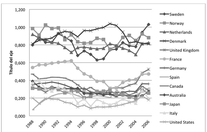
(9) The total net ODA disbursements, the aid data we will work with, are the sum of grants, capital subscriptions, total net loans and other long-term capital. Figure 1 shows the ratio of ODA over GDP for the most important donors from 1988 through 2007. The Nordic countries (Sweden, Norway, and Finland) and the Netherlands show the highest figures. Throughout this entire period, they consistently gave more than 0.6% of GDP as ODA and in some years the percentage surpassed 1 percent for the Netherlands. The USA presents the lowest figures showing percentages that are in many years below 0.2 percent of GDP. Figure 1. Donor’s ODA-to-GDP ratio (1988-2007) 3.2 Data Sources The datasets used are the following: ODA data from 1988 to 2007 are from the OECD Development Database on Aid from DAC Members. We consider bilateral net ODA disbursements in current US$7, instead of aid commitments, because we are interested in the funds actually released to the recipient countries in a given year. Disbursements record the actual international transfer of financial resources, or the transfer of goods or services valued at the cost to the donor. We also consider multilateral aid as a proxy for donors’ total contributions to multilateral aid and the percentage of tied aid with respect from total aid. The original DAC member countries are Australia, Austria, Belgium, Canada, Denmark, Finland, France, Germany, Ireland, Italy, Japan, Luxembourg, the Netherlands, New Zealand, Norway, Portugal, Sweden, Switzerland, the United Kingdom, and the United States. Other countries are also included in the data, but they became donors many years later: the Czech Republic (1998), Greece (1996), Hungary (2003), Iceland (1988), Korea (1989), Latvia (2002), Lithuania (2001), the Slovak Republic, Spain (1987), and Turkey (1990). In the empirical estimations we included all original DAC countries plus Greece and Spain. Bilateral exports are obtained from the UN COMTRADE database. Data on income and population variables are drawn from the World Bank (World Development Indicators Database, 2009). Bilateral exchange rates are from the IMF statistics. Distances between capitals have been computed as Great Circle distances using data on straight-line distances in kilometers, latitudes, and longitudes from the CIA World Fact Book. Other dummy variables included in the model are from CEPII8. The RTA variable has been constructed using the files provided by De Sousa (2012). Summary statistics of the described variables are presented in Table A.1 in the Appendix. 7 8. The net amount comprises total grants and loans extended (according to DAC). The Centre d'Etudes Prospectives et d'Informations Internationales. 8.

(10) 4. Model Specification and Results 4.1 Model Specification The gravity model of trade is nowadays the most commonly accepted framework to model bilateral trade flows. Solid theoretical foundations that provide a consistent base for empirical analysis have been developed in the past three decades for this model (Anderson, 1979; Bergstrand, 1985; Anderson and van Wincoop, 2003; Helpman, Melitz, and Rubinstein, 2008; Nelson and Juhasz Silva, 2012). The major contribution of Anderson and van Wincoop (2003)(AvW) was the appropriate modeling of trade costs to explain bilateral exports. According to the underlying theories, trade between two countries is explained by nominal incomes and the populations of the trading countries, by the distance between the economic centers of the exporter and importer, and by a number of trade impediment and facilitation variables. Dummy variables, such as trade agreements, common language, or a common border, are generally used to proxy for these factors. The gravity model has been widely used to investigate the role played by specific policy or geographical variables in explaining bilateral trade flows. Consistent with this approach, and in order to investigate the effect of development aid on donors’ exports, we augment the traditional model with bilateral and multilateral aid (ODA) variables. Among the variables facilitating trade, we add bilateral (tied and untied) and imputed multilateral aid. Introducing time variation and bilateral exchange rates9, the augmented gravity model is specified as α. α. X ijt = α 0 Yitα1Y jt 2 YHitα3YH αjt4 DISTij 5 BAIDijtα6 BAIDK αjt7 MAIDitjα8 EXCHRijtα9 Fijtα10 uijt. (1). where Xijt are the exports from donor i to recipient j in period t in current US$; Yit (Yjt) indicates the GDPs of the exporter (importer) in period t, YHit (YHjt) are exporter (importer) GDPs per capita in period t and DISTij is geographical distances between countries i and j. BAIDijt is bilateral official net development aid10 from donor i to country j in period t in current US$; and MAIDijt is imputed multilateral development aid from donor i to country j in period t in current US$; Fijt denotes other factors impeding or facilitating trade (e.g. RTAS, common language, a colonial relationship, or a common border). EXCHRijt denotes nominal bilateral exchange rates in units of local currency of country i (donor) per unit of currency in country j (recipient) in year t. Finally, uijt is an idiosyncratic error term that is assumed to be well behaved. Note that aid variables could be inserted with lags, in accordance with the theoretical predictions. 9. When the gravity model is estimated using panel data, it is recommended to add bilateral exchange rates, as well, as a control variable (Carrère, 2006). 10 We also distinguish between tied and untied aid in the estimations presented below. 9.

(11) Usually the model is estimated in log-linear form11. Taking logarithms in Equation 1, the specification of the gravity model is LX ijt = γ 0 + φt + α1 LYit + α 2 LY jt + α 3 LYH it + α 4 LYH jt + α 5 LDIST ij + α 6 LBAID ijt + α 7 LBAIDK jt +. α 8 LMAID ijt + α 9 LEXCHR ijt + α10CONTIG ij + α11COMLANG ij + α12COLONY ij + α13 RTAijt + ηijt. (2). where L denotes variables in natural logs, RTA, CONTIG, COMLANG, COLONY are dummies that take the value of one when countries belong to the same trade agreement, share a border, have the same official language or have a colonial relationship, respectively and the other explanatory variables are described above. φt are specific time effects that control for omitted variables common to all trade flows but which vary over time. In the estimations, the constant (γo) is replaced by a trading-pair specific intercept, δ ij , sometimes also referred to as dyadic fixed effects to control for unobservable bilateral effects that are time invariant. When these effects are specified as fixed effects, the influence of the variables that are time invariant and vary by trading pair cannot be directly estimated. This is the case for distance, common language, contiguity, and colonial history; therefore, its effect is subsumed into the country-pair dummies. Finally, ηijt is an idiosyncratic error term that is assumed to be well behaved. The model will be estimated for all donors and also for each donor separately by restricting the income and income-per-capita coefficients to being equal (α1 =α2 and α3=α4). To investigate the existence of the above-mentioned displacement effect, we use two additional control variables. First, aid from other donors (different from donor i to recipient j , LBAIDK=∑LBAIDkjt). The rationale of adding this variable is to control for cross-correlation effects due to the fact that other donors’ aid could promote their own exports to recipient j, which may have a negative effect on donor i‘s exports12. In our panel data framework, we do not think that endogeneity concerns will bias our results, as we are effectively investigating to what extent changes in aggregate aid flows of other donors affect exports from donor i; in any case, our robustness checks (GMM framework) would specifically address the endogeneity problem as well and confirm the validity of our results.13 Alternatively, as a robustness check we also use the share of total aid given to each recipient by other donors (LBAIDSHKjt). 11. We also estimate the model in its original multiplicative form. To our knowledge, this is the first paper to estimate this “crowding-out” effect in a multi-donor’s setting. Martínez-Zarzoso et al. (2009) found some evidence indicating that aid from other EU countries displace German exports, although that result was not robust. 13 In particular, the pair fixed effects are likely to capture all long-term bilateral trade relations, while the time fixed effects will capture effects common to all donors that vary over time. The only possible concern is that exports from donor i reduce aid flows from other bilateral donors. There is little evidence for such an effect in the literature or in our data; to the extent such an effect exists, it is captured in the lag structure we use as well as in the GMM framework. 10 12.

(12) This effect intends to capture the importance of donor i for a given aid recipient; in particular, if the share of other donor-giving is high, we would expect that this is more likely to crowdout exports from donor i. However, we find mainly insignificant results when using this variable and therefore we show results only with LBAIDK. Considering that it may take some time before aid fully affects trade, we include a number of lags of the two types of aid (bilateral and imputed multilateral) in the model specification. To determine the number of lags added to the right-hand side, we start by adding more lags than one could reasonably expect to need and then disregard those that are statistically non-significant. The chosen number of lags arrived using this procedure is two for bilateral aid and one for imputed multilateral aid. With respect to the specification of the country-pair effects, we not only consider the usual fixed-versus-random-effects approach, but also an attractive alternative approach, which is especially suitable when there are missing values and the time span is short, and consists of estimating the model, as proposed by Mundlak (1978), including within and between effects (Egger and Url, 2006). Basically, this approach involves modeling the correlation of unobserved heterogeneity under the assumption that the unobserved factors are correlated with the group mean of the explanatory variables. Each time-variant variable is included twice, once in its original form and once averaged over time. Feasible Generalized Least Squares (FGLS) on this model obtains both within effects and the between-within effects in a single model. According to Egger and Pfaffermayer (2004), the former approximate short-run effects, and the latter additional long-run effects. This model could be named correlated random effects model. The extended model is given by. LX ijt = γ 0 + φ t + α 1 LYit + α 2 LY jt + α 3 LYH it + α 4 LYH jt + α 5 LDIST ij + α 6 LBAID ijt + α 7 LBAIDK jt + α 8 LMAID ijt + + α 9 LEXCHR. ijt. + α 10 CONTIG ij + α 11COMLANG ij + α 12 COLONY ij + α 13 RTAijt + α 14 AVLYDij + α 15 AVLYRij +. α 16 AVLYHDij + α 17 AVLYHR ij +α 18 AVLBAIDij + α 19 AVLBAID j + α 20 AVLMAIDij + α 21 AVLEXCHRij +. (3). + α 22 AVRTAij + η ijt. where variables starting with AV refer to averages over time of the time-variant. where η ijt = µ ij + ν ijt. regressors that were described above. According to Mundlak (1978), the heterogeneity bias will be minimal, due to the fact that the correlation between the country-pair effects and the explanatory variables is captured in the model. FGLS estimation of model (3) will provide similar estimates to the within transformation and, therefore, unbiased estimates. Equation (3) is also estimated for groups of donors and for each donor country to account for country 11.

(13) heterogeneity. Indeed, the literature has argued that different donors may use aid in different ways (e.g. seeking new markets or reinforcing existing relationships) which predict opposite effects. In the next section, estimation results obtained with the outlined approaches are presented and discussed. 4.2. Main Results Model 3 is estimated for data on 21 donors’ exports and development aid (ODA) to 132 recipient countries during the period of 1988 to 2007. Table 1 reports the main estimation results for all donors. Table 1: Development Aid and Donors’ Exports—Results for different periods The correlated random effects model (model 3) is estimated with a flexible structure in the error term that allows for panel-specific variances and for first order autocorrelation within panels; the results for the whole period are shown in Column 1 (Table 1). This is our preferred specification14. A RESET-type test indicates that the model is correctly specified (last row in Table 1). The within-coefficients on bilateral and multilateral aid are practically unchanged with respect to those in the FE specification15. With respect to the variable of interest, bilateral aid, the estimated within-coefficient is always positive and significant, indicating that a one-percent increase in bilateral aid raises donors’ exports by 0.039 percent (0.021+0.011+0.07). The effect is smaller compared to that shown in previous studies which did not control for country-pair unobserved heterogeneity, autocorrelation, and heteroskedasticity, but it is still positive and significant. Using the results in Column 1 (Table 1), we find that, in the short run, the average return on aid for donors’ exports is approximately a $0.50 US increase16 in exports for every aid dollar spent. 17 14. Results of the most popular specifications are reported in the Appendix. The first and second columns of Table A.1 show the pooled OLS without and with lagged aid terms, respectively. Time-fixed effects are also included in both columns. Individual (country-pair) effects (modelled as random) are included in Column 3 to control for unobservable heterogeneous effects across trading partners. A Hausman test indicates that the dyadic unobservable effects are correlated with the error term, hence the random effects approach, ignoring this correlation, leads to inconsistent estimators. The fourth column presents the two-way FE estimates that are consistent. Restricting the analysis to the within variation eliminates the bias due to unobserved heterogeneity that is common to each trading-pair but means that the between-variation is lost. 15 The fixed effects results are available on request. 16 This average is calculated as: ∂X = β BAIDG * AV ( X ) = 0.039 * 276906 = 0.49 ∂BAIDG. 17. AV ( BAIDG). 22071. The fixed effects results obtained by Wagner (2003) implied that exports derived from a dollar of aid amount to $0.73 US for a sample of 20 donors, 108 recipients, and five years (1970, 1975, 1980, 1985, and 1990). This result, in the context of a static gravity model, is higher than our preferred result ($0.55 US using the coefficients of Model 1 in Table 1), but closer to the result obtained for the period 1988-1993 ($ 1.1 US). It seems that the average return to aid in terms of donors’ exports has been decreasing over time. However our results are not strictly comparable to Wagner (2003). Indeed, he did not control for autocorrelation and heteroskedasticity in the 12.

(14) It is worth noting that the between-effect (the coefficient obtained for bilateral aid averaged over time) is much larger in magnitude (0.209) than the within effect, and considering that it could be taken as an approximation of the long-run effect, using this result, the average return on aid for donors’ exports in the long term is approximately a $2.5 US increase in exports for every aid dollar spent. The estimated coefficient for the official net development aid of other donors is also positive and statistically significant, but the magnitude is quite low (0.012). This suggests that donors’ exports could be positively influenced by aid given by other DAC members. In particular, when other donors give higher amounts of aid to a particular recipient and aid is untied, it could promote recipient imports also from other donors, generating a positive effect on a specific donor’s exports. By adding these effects to the effect of bilateral aid from other donors, the average return on aid for donors’ exports amounts to $0.63 US increase in exports for every aid dollar spent. However, the between-coefficient of our displacement-variable is negative and significant indicating that higher average aid in the whole period from other donors to a given recipient decreases bilateral exports of a given donor. Subtracting this negative effect from the long-run effect of bilateral aid, the average return on aid for donors’ exports in the long term amounts to $1.9 US increase in exports for every aid dollar spent. With respect to multilateral aid, the within-effect on donors’ exports is positive and significant. According to column 1 (Table 1), an increase of 10 percent in multilateral aid increases exports by 0.022 (0.012+0.010) percent. Most of the other variables present the expected sign and are statistically significant and of similar magnitude as found in the literature. Columns 2-4 (Table 1) present the results for three different periods of time. For the first period (1988-1993) the total effect of bilateral aid on exports is higher than average, being the estimated elasticity 0.15, which corresponds to a $1.1 US18 increase in exports for every aid dollar spent. However the effect is reduced to a $0.5 US increase in exports for every aid dollar spent in the period 1994 to 2000 and fades away after 2000 (Column 4, Table 1). Interestingly, these decreasing aid-elasticities are accompanied by increase coefficients of the RTA variable, which is positive and statistically significant for the last two periods. In particular when a North-South trade agreement is in. error term and he included only data for five years during the 1970s and 1980s, whereas we examine the 1990s and the 2000s and use a wider sample of countries and years. 18. This increase ($ 1.1) is calculated as in footnote 13, that is multiplying the aid coefficient (0.15) by the ratio between average exports and average bilateral aid over the period 1988-1993. 13.

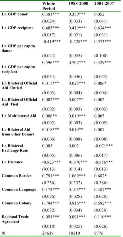
(15) place, donors export around 8 (12) percent more in the period 1994 to 1999 (2000-2007), whereas RTA is not statistically significant in 1988-1993. The decreasing effect of aid on donor’s exports could also be related to the 2001 DAC recommendation of untying official development assistance to least developed countries, which entered into force on 1 January 2002, and the Paris Declaration agreed in 2005, are having an effect on donor’s aid policies. Specifically, if the effect of aid on donor’s exports is related to tied aid, an increase in the amount of untied aid could reduce or even eliminate the effect. To investigate this hypothesis we separate untied and tied aid19 in the regressions to see what part of aid accounts for a larger effect. The results are shown in Table 2. Table 2. Development Aid and Donors’ Exports—Results Adding Tied Aid We divide the sample in two periods to account for the changes induced by the DAC recommendation of untying ODA (the second period starts in 2001 to account for an anticipation effect) and, for simplicity, we estimate a more parsimonious model (without lagged aid variables). The results indicate that only a small part of the aid effect is attributed to tied aid. The coefficient of tied aid is only statistically significant in the first period, whereas untied bilateral aid has a positive and significant effect on exports in both periods, but only at the ten percent level in 2001-2007; the size of the coefficient does not differ significantly which would suggest that tying does not have an impact on the export effects.. However, we suspect that the tying status suffers from measurement error for a number of reasons. First, the tying status is only available by donor but not bilaterally (donor-recipient). Second, some donors do not report the tying status for a number of years and the data are only available for aid commitments and not for disbursements. Finally and most important, we are not able to account for informal tying practices, which surely are linked to trade. Since the available data on tied aid does not allow us to accurately distinguish between tied and untied bilateral aid and in what follows we continue to use bilateral aid disbursements (BAID), as in Table 1, and we exploit instead the time variation of the estimated coefficients to infer the effect of tied versus untied aid on exports.. 19. Table DAC 7b (from OECD.Stat) is used to obtain the tying status of bilateral ODA commitments. Members have agreed that administrative costs and technical co-operation expenditure should be disregarded in assessing the percentages of tied, partially untied and untied aid. We calculate the percentage of tied aid over total aid and assume that the same percentages apply to aid disbursements. 14.

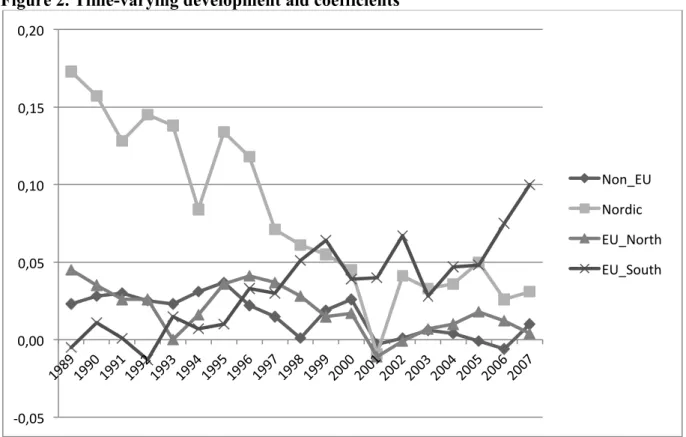
(16) Next, to account for possible heterogeneity of the estimated coefficients across donors, Figure 2 presents separated results for groups of donors obtained by using the correlated random effects estimator and allowing the bilateral aid coefficients to vary over time. Figure 2: Development Aid and Donors’ Exports— Results for Groups of Donors We have classified donors according to geographical location and to the economic blocs to which they belong. We are aware of the fact that it is an ad-hoc classification and other criteria could also be valid, for this reason we also present individual donor regressions. The main reason for grouping the donors is that we are able to efficiently estimate time-varying aid coefficients. Looking at the aid coefficients, a clear decreasing pattern is observed for most groups of donors over time, with the only exception of EU- South (periphery) countries. Most of these countries, apart from Italy, started to give development aid in the late 1980s and early 1990s. The most pronounced decline in the aid elasticity is shown for the group of Nordic countries, which includes Denmark, Finland, Norway and Sweden, with aid coefficients that are not statistically significant in the 2000s. But also for EU-North (Austria, Belgium, France, Netherland, Germany, UK) and Non-EU (Australia, Canada, Japan, New Zealand, Switzerland, US), the effect of bilateral aid on trade vanishes in the 2000s. Only for EU Southern countries the pattern is different showing increasing and significant aid elasticities in the 2000s. It is also worth noting that for EU countries ( EU-North and EUSouth groups) aid given by other donors (BAIDK) shows as negative effect on exports of a given donor, showing a displacement effect that may reduce the return of aid on bilateral exports (Martinez-Zarzoso et al. 2009 also found a similar displacement effect for the German case). Finally, Table 3 shows the average effects of bilateral aid on exports for each donor. Aid elasticities vary among donors20, with Australia, Germany, Italy, Spain and Sweden showing above-average effects. It is also found that for six countries—Belgium, Finland, Greece, Ireland, the Netherlands, New Zealand, Portugal and Switzerland —such effects are –on average and for the whole period– not statistically significant. It is worth mentioning that. 20. The slightly lower effect found for Germany in comparison to Martínez-Zarzoso et al. (2009) and Nowak Lehmann D. et al. (2009) is probably due to the longer and different time period considered in those studies (1960-2004). And it is consistent with our findings pointing to a decrease in the effect of aid on donor’s exports over time. 15.

(17) Greece, Portugal and Ireland began giving aid in the 1990s and so the number of observations for them is lower than that for other donors, which could render the results insignificant. Table 3: Development Aid and Donors’ Exports—Results for Each Donor Table 3 also presents the short-run monetary return on aid from single donors’ exports. One US dollar spent on aid generates more than fifty cents (US$) of exports for Australia, Austria, Germany, Italy, Spain, and Sweden. The highest return is found for Australia. We also run single-donor regressions using alternative estimators. According to the results of the two-way FE within estimator21, the average effect, calculated as the average of the estimated coefficients in single donor regressions, is similar to the one found in Table 3 and is close to the average effect obtained in column 1 (Table 1). 4.3 Robustness Checks A battery of robustness check supports our results and competing specifications indicate that our estimates are conservative. As a first robustness check, we consider an alternative specification that includes country-and-time effects to account for time-variant, multilateral price terms, as proposed by Baldwin and Taglioni (2006) and Baier and Bergstrand (2007). As stated by Baldwin and Taglioni, including time-varying country dummies should completely eliminate the bias stemming from the “gold-medal error” (the incorrect specification or omission of the terms that Anderson and van Wincoop (2003) called multilateral trade resistance). Income and income-per-capita variables cannot be estimated because they are collinear with the exporter and time variables and importer and time multilateral resistance terms. Bilateral fixed effects are also included to isolate the aid impacts on bilateral trade flows from any time-invariant country-pair-specific elements, some of which (colonial links, common language) could be related to the decision on giving aid. In this way we are also able to partially account for the aid endogeneity issue. Table A.2 provides results for three periods including time-varying country dummies. The two-way fixed effect within-estimator with robust and clustered standard errors has been used and only the level of the ODA variables enter the model, since the two lags of ODA were not statistically significant. The estimated coefficients for the impact of bilateral ODA on exports are decreasing over time (from column 1 to 3) and lie within the interval (0.023-0.053) until 21. Results are available upon request from the authors. 16.

(18) 2000. Compared with the average results obtained in Table 1 (column 1), the results are very similar on average (0.038). ODA also turns out to be insignificant from 2000 onwards22. Simultaneously, we find a clear displacement effect since 2001 onwards, indicating that an increase of 10 percent in other donors’ aid leads to a decrease of 1.28 percent in bilateral exports of a particular donor to the given recipient. Hence, there is a displacement effect that may indirectly induce increases in other donors’ exports to the detriment of a given donor’ exports. The results were very similar when the share of aid was added instead of the magnitude. Second, two issues related to the estimation of gravity models of trade that may give raise to biased estimates are the presence of zeros in the dependent variable (bilateral trade) and the omission of the extensive margin of trade (number of exporters). To approach these issues we consider an alternative specification that is based on Helpman et al. (2008). Table A.3 presents the results from estimating Equation 3 (Mundlak approach), first considering only selection effects, showing the results of the second step estimation in the first column of Table A.3, and second, considering selection effects and heterogeneity in productivity, with the results of the second step estimation given in column 2 (Table A.3). In the first-step estimation, we estimate a correlated random-effects probit model with time effects. The selection variable used is the variable corruption. Hence this variable is excluded in the second step estimations23. From these estimates we obtained the inverse Mills ratio (INVMILLS) and the linear predictions down-weighted by their standard error (ZHAT) and these two elements were incorporated as regressors in the second-step estimation. Column 2 in Table A.3 incorporates into the second-step estimation heterogeneity in productivity and self-selection effects, along with random effects, average effects of the time-variant variables and time dummies. Both, the ZHAT coefficient and the INVMILLS coefficient are not statistically significant, showing no evidence of selection effects or heterogeneity in productivity. Hence, disregarding selection effects and heterogeneity in productivity does not change the estimates.24 Next, we estimate a dynamic gravity model following the standard technique of adding lagged dependent variables as regressors. The results for three different sub-periods are 22. We also performed sequential estimations adding a year at a time and aid started to be insignificantly related to exports from 2000 onwards. It thus appears that the export-enhancing effect does get smaller over time, which could be related to changes in aid allocation (focusing on poorer countries) and less tying of aid post-2000, following recommendations of OECD-DAC on aid effectiveness. 23 Other studies used religion or legal origin as exclusion variables, but in general the results are unchanged. 24 Note that Helpman et al. (2008) and Johansson and Pettersson (2012) find the selection bias to be economically negligible. 17.

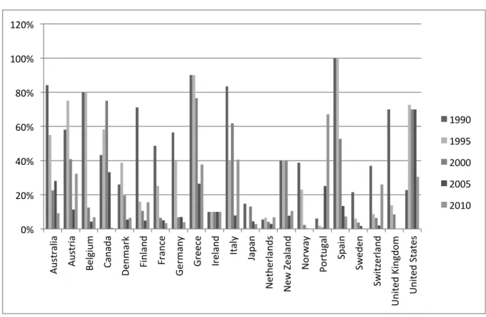
(19) presented in Table A.4. The first three columns in this table present the results obtained by following a difference GMM approach for the same three periods as in Table A.2 (1988-1993, 1994-2000, 2001-2007), while Columns 4 to 6 present the results when estimating by the system GMM approach25. This second method is commonly accepted as one of the ways to estimate the determinants of bilateral export flows in a dynamic context. The results concerning the variable of interest obtained in Columns 4 to 6 are consistent with those obtained above. Indeed, the average return on aid for donors’ exports in the long term, calculated using the average of the long-term aid coefficients in those periods, is approximately a $1.88 US increase in exports for every aid dollar spent, which is slightly lower than the estimate found in the correlated random effects model ($1.9 US increase after subtracting the displacement effect). In this framework we also tested for endogeneity of bilateral aid and for non-linearities. Aid is found to be exogenous and the squared coefficient of bilateral aid reinforces the effect of aidi. 5. Discussion of the Results and Policy Implications To better understand the reasons why the effect of bilateral aid on bilateral exports has decreased over time and affects differently each donor’s exports, we look at the tying status of aid over time and for different donors. Figure 3 shows the time-evolution of tying status of aid for each single donor. Figure 3. Tying status of development aid across donors and over time With respect to the tying status, despite the DAC recommendations of untying ODA given in 1987, 2002 and 2005, In 2006, Austria and Canada still tied 19 and 34 percent of its ODA, US and Spain around 19 and 54 percent and Australia 36.8 percent (in 2005)26. . Figures reported in Table 3 indicate that all these donors show a higher than average return to aid. Although previous research (Jepma, 1991) stated that tied aid was not more exportpromoting for donors than non-tied aid, this could be different according to more recent data. 25. The models estimated using Difference-GMM and system-GMM estimators pass the specification tests: autocorrelation of second order is rejected and the Hansen over-identification test indicates that the validity of the instruments cannot be rejected. However, in two cases we have to add a second lag of the dependent variable to the baseline specification.. 26. Although in 2006 Australia officially untied most of its aid (nationally-tied aid), the informal tying of aid continues today with Australian companies receiving the majority of aid contracts (http://aidwatch.org.au/whereis-your-aid-money-going/australian-government-aid/australian-aid-priorities/tied-aid).. 18.

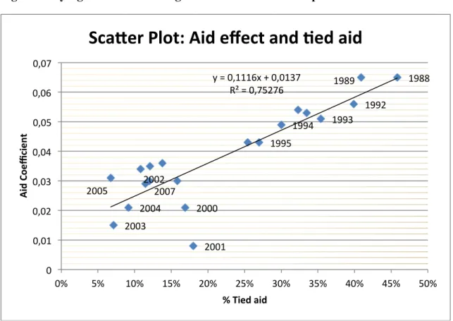
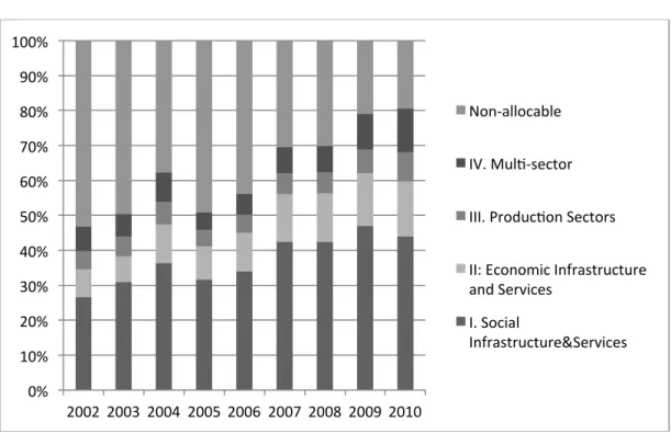
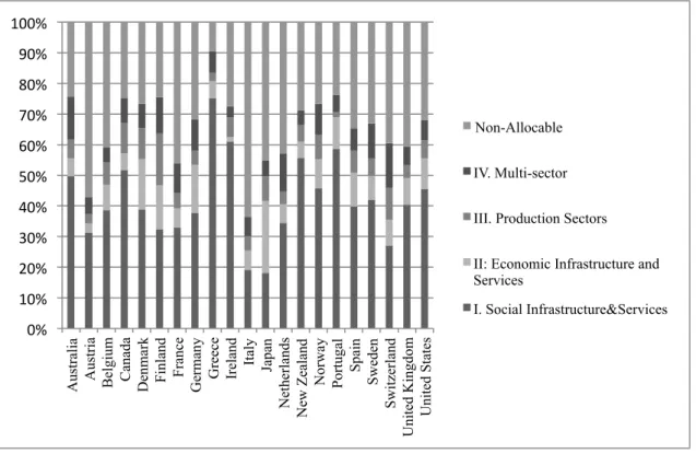
(20) Indeed, donors with a higher share of tied aid appear to have a higher return to aid in terms of exports. The importance of tied aid would also explain the falling export-promoting effect of aid post-2000 after which tying of aid (formal and informal) has been much reduced. This evidence is more clearly shown in Figure 4, which shows the average effect of aid on exports by year and relates that to the average tying of aid each year. It points towards a positive correlation between the aid effect and the tying status over time. Fitting a simple OLS regression, the tying status explains 75 percent of the variation of the aid coefficient. Figure 4. Tying status and aid effect on exports. A similar OLS regression across donors, where we examine the average tying status of aid over time for individual donors, and relate that to the average effect of aid on exports from each donor indicates that the tying status explains around 25 percent of the across-country variation of the aid coefficients. This confirms that tying appears to play a modest role in explaining the differing aid effects on donor exports between different donors. And it is also likely to contribute to the declining export effects of aid for all donors. Indeed, other factors may play a role, as for example the sectoral allocation of development aid, which has changed over time and significantly differs across donors. More specifically, Figure 5 shows that the percentage of sectoral allocable aid has increased over time –on average– for all donors, for instance more sharply for EU Northern countries27. Since this information is only available from 2002 onwards we cannot report statistics for our sample period. Figure 6 reports instead average figures for the period 2002-2010 of how individual donors allocated their aid to different sectors. We will relate this evidence to our results concerning the aid effects. Figure 5. Sectoral allocation of development aid Figure 6. Sectoral allocation of development aid across donors On average, over the period 2002-2010 most donors with a non-significant aid-trade effect (Belgium, Finland, Greece, Ireland, the Netherland, New Zealand, Portugal) dedicate more than 30 percent of its aid to social infrastructure and services (Greece, Ireland and Portugal and New Zealand more than 50 percent). These are all donors showing a significant aid-trade link, as well as donors that dedicate an important share of their ODA to production sectors like Canada and Denmark or donors for which a high aid share is classified as “non. 27. This is not shown in Figure 5, available upon request. 19.

(21) allocable aid”28, like Austria, France, Italy, and Japan with more than 40 percent. However, this evidence is not enough to conclude that sectoral allocation of aid is affecting the relationship between aid and donors’ exports. We conclude that whereas the tying status of aid seems to be correlated to the magnitude of the effect of aid on exports,. the donors’. differences in sectoral allocation show a very mixed picture that seems to be only partially related to the effect of aid on donor’s exports. We suspect that a more detailed disaggregation would be required to assess the impact of sectoral allocations on the aid-export link more fully. In summary, our results indicate that in the short run the average return on aid for donors’ exports in the period 1988-2007 is approximately a $0.50 US dollar increase in exports for every aid dollar spent, whereas in the long run, this number is even larger (around $ 1.8 USdollar). However, this result shows an average effect that has been decreasing over time and disappeared in the 2000s for most donors and it is also very different across donors, with later members of the DAC showing a different picture. 6. Conclusions The purpose of this paper is to analyze the effects of development aid on donors’ exports. The study period runs from 1988 to 2007. The main results can be summarized as follows. First, donors’ bilateral aid has positively affected their exports to developing countries. The results point to large beneficial effects of bilateral aid on donor’s exports and to non-negligible effects of multilateral aid in the short term. Second, the effects of bilateral aid on exports vary over time and across donors. Indeed, the effects of aid on donors’ exports do appear to have decreased substantially over the period studied. Among donors, Australia, Italy, Germany, Spain and Sweden showing the greatest positive effects; this appears to be related to differences in the tying status and in the sectoral allocation of aid. Third, a particular donor’s export levels were negatively affected if other donors increased their aid, only for EU donors. It is worth noticing that the effect of bilateral aid on trade is even not statistically significant in the 2000s, showing perhaps an effect of the recommendations given by the DAC concerning the tying of aid and differences in sectoral aid allocation. While we do not assess the various transmission channels directly, the findings are consistent with the notion that in the last decades bilateral aid has promoted exports from donor to recipient countries, 28. We consider in this category other aid classified as: commodity aid, action related to debt, administrative cost of donors and unallocated aid. 20.

(22) has promoted export-enhancing goodwill and exposure, and displaced exports from other donors, at least in some cases. These results could be good news for both developing and developed countries. The first could benefit from receiving more productive aid. The second could contribute to the economic development of poor countries by focusing on the best aim of development aid, which is improving the living conditions of developing countries and use other means of promoting trade, namely RTAs, trade missions and other trade promotion policies that do not have detrimental effects on developing countries’ economic performance.. 21.

(23) REFERENCES Alesina, A. and Dollar, D. (2000). Who Gives Aid to Whom and Why?. Journal of Economic Growth. 5: 33-63. Anderson, J. E. (1979). A Theoretical Foundation for the Gravity Equation. American Economic Review. 69: 106-116. Anderson, J.E. and Van Wincoop, E. (2003). Gravity with Gravitas: A Solution to the Border Puzzle. American Economic Review. 93: 170-192. Arvin, M. and Baum, C. (1997). Tied and untied foreign aid: Theoretical and empirical analysis. Keio Economic Studies, 34(2), 71-79. Arvin, M. and Choudry, S. (1997). Untied aid and exports: Do untied disbursements create goodwill for donor exports?. Canadian Journal of Development Studies, 18(1): 9-22. Baier, S. L. and Bergstrand, J. H. (2007). Do Free Trade Agreements Actually Increase Members’ International Trade. Journal of International Economics. 71: 72-95. Baldwin, R. and Taglioni, D. (2006). Gravity for Dummies and Dummies for Gravity Equations. National Bureau of Economic Research Working Paper, 12516, Cambridge. Bergstrand, J.H. (1985). The Gravity Equation in International Trade: Some Microeconomic Foundations and Empirical Evidence. The Review of Economics and Statistics. 67:474481. Bergstrand, J. H. (1989). The Generalized Gravity Equation, Monopolistic Competition, and the Factor-Proportions Theory in International Trade. The Review of Economics and Statistics. 71: 143-153. Bhagwati, J. N., Brecher, R. and Hatta, T. (1983). The Generalized Theory of Transfers and Welfare: Bilateral Transfers in a Multilateral World. American Economic Review. 73: 606-618. Bhagwati, J.N., Brecher, R.A., and Hatta, T. (1984). The Paradoxes of Immiserizing Growth and Donor-Enriching ‘Recipient-Immiserizing’ Transfers: A Tale of Two Literatures. Weltwirtschaftliches Archiv. 120: 228-243. Brecher, R. A. and Bhagwati, J. N. (1981). Foreign Ownership and the Theory of Trade and Welfare. Journal of Political Economy. 89: 497-511. Brecher, R. A. and Bhagwati, J. N. (1982). Immiserizing Transfers from Abroad. Journal of International Economics. 13: 353-64. Busse, M., Hoekstra, R. and Königer, J. (2012). The Impact of Aid for Trade Facilitation on the Costs of Trading. Kyklos. 65: 143–163. Calí, M. and Te Velde, D.W. (2011). Does Aid for Trade Really Improve Trade Performance?. World Development. 39(5): 725-740. Carrère, C. (2006). Revisiting the effects of regional trade agreements on trade flows with proper specification of the gravity model. European Economic Review. 50 (2): 223247. De Sousa, J. (2012). The Currency Union Effect on Trade is Decreasing over Time. Economics Letters. 117(3): 917-920. Djajic, S., Lahiri, S. and Raimondos-Moller, P. (2004). Logic of Aid in an Intertemporal Setting, Review of International Economics. 12: 151-161. Doucouliagos, H. and Paldam, M. (2006). Aid Effectiveness on Accumulation: A Meta Study. Kyklos. 59: 227–254. Egger, P. and M. Pfaffermayer (2004). Estimating Long and Short Run Effects in Static Panel Models, Econometric Reviews. 23 (3): 199-214. Egger, P. and T. Url (2006). Public Export Credit Guarantees and Foreign Trade Structure: Evidence from Austria, The World Economy. 29 (4): 399-418. 22.

(24) Gale, D. (1974). Exchange Equilibrium and Coalitions: An example, Journal of Mathematical Economics. 1: 63-66. Head, K. and Ries, J. (2010). Do Trade Missions Increase Trade?, Canadian Journal of Economics. 43(3): 754-775. Helpman, E. & Melitz, M. & Rubinstein, Y. (2008). Estimating Trade Flows: Trading Partners and Trading Volumes. The Quarterly Journal of Economics. MIT Press, 123(2): 441-487. Jepma, C. (1991). The tying of aid. Organization of Economic Cooperation and Development Paris. Johansson, L.M. and Pettersson, J. (2013). Aid, Aid for Trade and Bilateral Trade: An Empirical Study. Journal of International Trade and Economic Development. 22 (6): 866-894. Keynes, J. M. (1929c). Mr. Keynes’ Views on the Transfer Problem. The Economic Journal. 39: 388-408. Leontieff, W. (1936). Note on the Pure Theory of Capital Transfer. In: Explorations in Economics: Notes and Essays Contributed in Honor of F. W. Taussig, McGraw-Hill Book Company, New York. Lloyd, T.A., McGillivray, M., Morrissey, O., and Osei, R. (2000). Does Aid Create Trade? An Investigation for European Donors and African Recipients, European Journal of Development Research. 12: 1-16. Martínez-Zarzoso, I. and Nowak-Lehmann D., F. (2003). Augmented Gravity Model: An Empirical Application to Mercosur-European Union Trade Flows, Journal of Applied Economics. VI (2): 269-294. Martínez-Zarzoso, I., Nowak-Lehmann D., F., Klasen, S. and Larch, M. (2009). Does German Development Aid Promote German Exports?. German Economic Review. 10 (3): 317338. Martínez-Zarzoso, I., Nowak-Lehmann D. and Horsewood, N. (2009). Are Regional Trading Agreements Beneficial? Static and Dynamic Panel Gravity Models. North American Journal of Economics and Finance. 20: 46-65. Martínez-Zarzoso, I., Nowak-Lehmann D. and Johannsen, F. (2012). Foreign Aid, Exports and Development in Euromed. Middle East Development Journal. 4 (2): 1-24. Martínez-Zarzoso, I., Nowak-Lehmann D. F. and Klasen, S. (2014). Aid and Donor’s Exports –The Dutch Case. Department of Economics. University of Goettingen. Mimeo. Morrissey, O. (2006). Aid or Trade, or Aid and Trade?. The Australian Economic Review. 39: 78–88. Mundlak, Y. (1978). On the Pooling of Time Series Data and Cross-section Data. Econometrica. 46: 69-85. Nelson, D. and Juhasz Silva, S. (2012). Does Aid Cause Trade? Evidence from an Asymmetric Gravity Model. The World Economy. 35 (5): 545-577. Nilsson, L. (1997). Aid and Donor Exports: The Case of the EU Countries, in: Nilsson, L., Essays on North-South Trade. Lund Economic Studies 70, Lund. Nowak-Lehmann D., F., Martínez-Zarzoso, I., Klasen, S and Herzer, D. (2009). Aid and Trade: A Donor’s Perspective. Journal of Development Studies. 45 (7): 1-19. Nowak-Lehmann D., F., Martínez-Zarzoso, I., Klasen, S, Herzer, D. and Cardoso, A. (2013). Does Foreign Aid Promote Recipient Exports to Donor Countries?. Review of World Economics. 149 (3): 505-535. Organization of Economic Cooperation and Development (2008). Development Co-Operation Report 2007, OECD Journal on Development, OECD, Paris. Portugal-Perez, A. and Wilson, J. (2009). Why Trade Facilitation Matters to Africa. World Trade Review. 8(3): 379-416. 23.

(25) Rose, A. K. (2007). The Foreign Service and Foreign Trade: Embassies as Export Promotion. World Economy. 30: 22–38. Suwa-Eisenmann, A. and Thierry Verdier (2007). Aid and Trade. Oxford Review of Economic Policy. 23(3): 481-507. Younas, J. (2008). Motivation for Bilateral Aid Allocation: Altruism or Trade Benefits. European Journal of Political Economy. 24 (3): 661-74.. Wagner, D. (2003). Aid and Trade: An Empirical Study. Journal of the Japanese and International Economies. 17: 153-173. World Bank (2009). World Development Indicators 2009 CD-ROM, Washington, DC. Zarin-Nejadan, M., Monteiro, J. A. and Noormamode, S. (2008). The Impact of Official Development Assistance on Donor Country Exports: Some Empirical Evidence for Switzerland, Institute for Research in Economics (Irene), University of Neuchâtel, Switzerland.. 24.

(26) FIGURES Figure 1. Donors ODA-to-GDP ratio (1988-2007). 1,200 . Sweden Norway . 1,000 . Netherlands Denmark . Título del eje . 0,800 . United Kingdom France . 0,600 . Germany Spain . 0,400 . Canada Australia . 0,200 . Japan Italy . 0,000 . United States . Source: OECD International Development Statistics (IDS) online databases on aid.. 25.

(27) Figure 2. Time-varying development aid coefficients 0,20 . 0,15 . Non_EU . 0,10 . Nordic EU_North 0,05 . EU_South . 0,00 . -‐0,05 . Source: Regression results in Table 2. Non EU: Australia, Canada, Japan, New Zealand, Switzerland, US. Nordic: Denmark, Finland, Sweden, Norway. EU North: Austria, Belgium, France, Netherland, Germany, UK. EU South: Greece, Ireland, Italy, Portugal, Spain.. 26.

(28) Figure 3. Tying status of development aid across donors and over time 120% 100% 80% 1990 . 60% . 1995 40% . 2000 2005 . 20% . United States . United Kingdom . Switzerland . Sweden . Spain . Portugal . Norway . New Zealand . Netherlands . Japan . Italy . Ireland . Greece . Germany . France . Finland . Denmark . Canada . Belgium . Austria . Australia . 0% . 2010 . Source: OECD International Development Statistics (IDS) online databases on aid. Based on aid commitments.. 27.

(29) Figure 4. Tying status and average aid effect on donors exports over time. Sca4er Plot: Aid eﬀect and 9ed aid 0,07 y = 0,1116x + 0,0137 R² = 0,75276 . 0,06 . 1992 . 0,05 Aid Coeﬃcient . 1988 . 1989 . 1994 . 1993 . 1995 . 0,04 0,03 . 2005 . 2002 2007 2004 . 0,02 . 2000 . 2003 0,01 . 2001 . 0 0% . 5% . 10% . 15% . 20% . 25% . 30% . 35% . 40% . 45% . 50% . % Tied aid . Source: OECD International Development Statistics (IDS) online databases on aid and regression results.. 28.

(30) Figure 5. Sectoral allocation of development aid 100% 90% Non-‐allocable . 80% 70% . IV. Mul\-‐sector . 60% 50% . III. Produc\on Sectors . 40% . II: Economic Infrastructure and Services . 30% 20% . I. Social Infrastructure&Services . 10% 0% 2002 2003 2004 2005 2006 2007 2008 2009 2010 . Note: Figure 5 shows the percentage of bilateral sector allocable aid (I-IV) for the period 2002-2010. Source: OECD International Development Statistics (IDS) online databases on aid.. 29.

(31) Figure 6. Sectoral allocation of development aid across donors. 100% 90% 80% 70% . Non-Allocable. 60% IV. Multi-sector. 50% 40% . III. Production Sectors. 30% II: Economic Infrastructure and Services. 20% 10% . I. Social Infrastructure&Services Australia Austria Belgium Canada Denmark Finland France Germany Greece Ireland Italy Japan Netherlands New Zealand Norway Portugal Spain Sweden Switzerland United Kingdom United States. 0% . Note: The percentages shown in Figure 6 are averages over the period 2002-2010. Source: OECD International Development Statistics (IDS) online databases on aid.. 30.

(32) Table 1: Development aid and donors’ exports–results for different periods Whole Period 0.303***. 19881993 0.068. 1994-2000. 2001-2007. 0.394***. 0.066*. (0.025). (0.060). (0.042). (0.040). 0.479***. 0.045. 0.592***. 0.631***. (0.019). (0.033). (0.029). (0.030). -0.462***. 0.158. -0.426***. 0.365***. (0.046). (0.145). (0.064). (0.097). 0.663***. 1.165***. 0.372***. 0.332***. (0.039). (0.067). (0.062). (0.055). 0.021***. 0.063***. 0.025***. 0.003. (0.003). (0.006). (0.004). (0.003). 0.011***. 0.047***. 0.008*. -0.004. (0.003). (0.005). (0.004). (0.003). 0.007***. 0.041***. 0.003. -0.002. (0.002). (0.006). (0.004). (0.003). 0.012***. 0.034***. 0.020***. -0.003. (0.003). (0.007). (0.004). (0.004). 0.010***. -0.002. 0.025***. -0.006. (0.003). (0.007). (0.004). (0.004). 0.012**. 0.024**. -0.008. -0.001. (0.005). (0.011). (0.011). (0.007). 0.012*. 0.123***. 0.025***. -0.095***. (0.006). (0.013). (0.009). (0.018). -0.821***. -1.009***. -0.862***. -0.864***. (0.012). (0.019). (0.015). (0.013). 0.988***. 1.365***. 1.183***. 0.967***. (0.196). (0.152). (0.296). (0.293). 0.216***. -0.293***. 0.153***. 0.361***. (0.024). (0.032). (0.027). (0.028). 0.658***. 0.903***. 0.826***. 0.604***. (0.030). (0.035). (0.035). (0.034). 0.089***. -0.059. 0.076***. 0.113***. (0.017). (0.071). (0.025). (0.022). 0.209***. 0.145***. 0.201***. 0.229***. (0.007). (0.010). (0.010). (0.009). -0.058***. -0.085***. -0.011. -0.051***. (0.011). (0.016). (0.016). (0.014). Number of Observations. 25878. 4300. 11676. 11209. RESET Test (p-value). 0.144. Variables Ln GDP donor Ln GDP recipient. Ln GDP per capita donor. Ln GDP per capita recipient Ln Bilateral Official Aid Ln Bilateral Official Aid (t-1) Ln Bilateral Official Aid (t-2) Ln Multilateral Aid Ln Multilateral Aid (t-1) Ln Bilateral Aid from other Donors Ln Bilateral Exchange Rate Ln Distance Common Border Common Language Common Colony Regional Trade Agrement Average Ln Bilateral Official Aid Average Ln Bilateral Aid from other Donors. Note: * p<0.10, ** p<0.05, *** p<0.01. The dependent variable is bilateral exports at current prices. Coefficients for average values of the time variant variables (excluding aid) are omitted. t-statistics are reported. Reset reports the p-value of a Ramsey Reset specification test, which H0 is that the model is correctly specified. H0 cannot be rejected. Estimation method: correlated random effects.. 31.

(33) Table 2. Development aid and donors’ exports–results adding tied aid. Ln GDP donor Ln GDP recipient. Ln GDP per capita donor. Ln GDP per capita recipient Ln Bilateral Official Aid Untied Ln Bilateral Official Aid Tied Ln Multilateral Aid Ln Bilateral Aid from other Donors Ln Bilateral Exchange Rate Ln Distance Common Border Common Language Common Colony Regional Trade Agrement. Whole Period 0.381***. 1988-2000. 2001-2007. 0.350***. 0.052. (0.024). (0.033). (0.041). 0.485***. 0.419***. 0.634***. (0.017). (0.021). (0.031). -0.419***. -0.528***. 0.573***. (0.044). (0.055). (0.100). 0.596***. 0.702***. 0.329***. (0.034). (0.046). (0.055). 0.017***. 0.025***. 0.006*. (0.003). (0.004). (0.004). 0.007***. 0.007**. 0.002. (0.002). (0.003). (0.003). 0.006**. 0.010***. 0.005. (0.002). (0.003). (0.005). 0.018***. 0.019**. 0.007. (0.006). (0.008). (0.008). 0.005. 0.002. -0.071***. (0.005). (0.006). (0.017). -0.823***. -0.870***. -0.856***. (0.013). (0.014). (0.013). 0.791***. 1.069***. 0.682*. (0.256). (0.332). (0.386). 0.174***. 0.105***. 0.387***. (0.026). (0.028). (0.028). 0.794***. 0.916***. 0.592***. (0.032). (0.034). (0.036). 0.091***. 0.091***. 0.110***. (0.018). (0.025). (0.026). N 24639 10310 9776 Note: * p<0.10, ** p<0.05, *** p<0.01. The dependent variable is bilateral exports at current prices; the same control variables as in Table 1 are added to the regressions. LBAID is spitted into: LBAID_UNT is the natural log of untied net bilateral aid from donor i to country j and LTIED is the natural log of tied net bilateral aid from donor i to country j. Coefficients for average values of the time variant variables are omitted. Estimation method: correlated random effects.. 32.

(34) Table 3. Development aid and donors’ exports–results for each donor Correlated RE. LBAID. LBAID (-1). Return $1 US Aid in $X. NOBS. Australia. 0.045**. 0.023. 1.008. 854. Austria. 0.036**. 0.011. 0.480. 1095. Belgium. 0.009. -0.007. -. 1263. Canada. 0.058***. -0.006. 0.643. 1711. Denmark. 0.044***. 0.013. 0.134. 1158. Finland. -0.003. 0.017. -. 1188. France. 0.032**. 0.009. 0.293. 1917. Germany. 0.043***. 0.020*. 0.971. 1889. Greece. 0.001. 0.006. -. 492. Ireland. -0.012. 0.012. -. 1002. Italy. 0.021***. 0.018***. 0.917. 1505. Japan. 0.034***. 0.012. 0.432. 1934. Netherland. 0.012. 0.001. -. 1743. New Zealand. 0.001. -0.023. -. 738. Norway. 0.085***. 0.022. 0.248. 1495. Portugal. 0.024. 0.019. -. 255. Spain. 0.030***. 0.020**. 0.590. 1268. Sweden. 0.044***. 0.028**. 0.590. 1488. Switzerland. 0.006. 0.00. -. 1532. UK. 0.006. 0.020***. 0.247. 1632. US. 0.016**. 0.004. 0.353. 1661. Average. 0.025. 0.010. 0.516. . Note: * p<0.10, ** p<0.05, *** p<0.01 The dependent variable is bilateral exports at current prices, LBAID is net bilateral aid from donor i to country j. The return on aid is calculated using the results from columns 1 and 2, taking into account only the estimates that are significant at the 1, 5 or 10% level.. 33.

(35)