A new bi parametric family of temporal transformations to improve the integration algorithms in the study of the orbital motion

Texto completo

(1)A new bi-parametric family of temporal transformations to improve the integration algorithms in the study of the orbital motion José A. López Ortı́∗ †1 , Vicente Agost Gómez † , and Miguel Barreda Rochera† † Departamento de Matemáticas. Universidad Jaume I. Av Sos Baynat s/n 12071 Castellón. Spain. Abstract One of the fundamental problems in celestial mechanics is the study of the orbital motion of the bodies in the solar system. This study can be performed through analytical and numerical methods. Analytical methods are based on the well-known two-body problem; it is an integrable problem and its solution can be related to six constants called orbital elements. To obtain the solution of the perturbed problem, we can replace the constants of the two-body problem with the osculating elements given by the Lagrange planetary equations. Numerical methods are based on the direct integration of the motion equations. To test these methods we use the model of the two-body problem with high eccentricity. In this paper we define a new family of anomalies depending on two parameters that includes the most common anomalies. This family allows to obtain more compact developments to be used in analytical series. This family can be also used to improve the efficiency of the numerical methods because defines a more suitable point distribution with the dynamics of the two-body problem. Keywords: Celestial mechanics. Ordinary differential equations. Computational algebra. 2000 MSC: 70F05, 70F10, 70F15,70M20.. 1. Introduction One of the most important problems in celestial mechanics is the study of the orbital motion around a central body. This problem includes the planetary theories and the study of the motion of artificial satellites around the Earth. The problem of the motion of a planet around the Sun or an artificial satellite around the Earth can be modelized by means of the second order differential equations !r d2!r ! + F! = −µ 3 − ∇U (1) 2 dt r. Preprint submitted to Journal of Computational and Applied MathematicsDecember 2, 2015.

(2) where !r is the radius vector referred to the primary (the Sun in the case of a planet or the Earth in the case of an artificial satellite), G the gravitational constant, m the mass of the primary, m" the mass of the secondary (planet or artificial satellite), µ = G(m+ m" ) the spaceflight constant, U the potential that induces the conservative perturbation forces such as the gravitational forces; and F! represents the non conservative disturbing forces as the atmospheric friction, the radiation pressure, the solar wind, etc. The most important motion in the solar system can be described in its first approximation without considering the disturbing forces, as a two-body problem: Sun-planet, Earth-satellite, etc. The two-body problem is a well-known integrable problem and its solution is given by a set of the orbital elements !σ [15], [6], [1]. The most common set of elements is the third set of Brower and Clemence !σ = (a, e, i, Ω, ω, M ) [1], M = n(t − t0 ) + M0 , where n = µ1/2 a−3/2 is the mean motion and M0 is the mean anomaly in the initial epoch. To solve the motion problem there are two main ways: the analytical methods and the numerical methods. Analytical methods to solve the perturbed problem can be appropriate in case of the study of the planetary motion. In this case, the description of the perturbed motion can be obtained by means of the perturbation theory. This method is based on the Lagrange variation of constants and for each planet the variation of the elements is described by the Lagrange planetary equations [9] da dt de dt di dt dΩ dt dω dt dε dt. = = = = = =. 2 ∂R na√∂σ 1 − e2 ∂R 1 − e2 ∂R − + na2 e ∂ω na2 e ∂σ ∂R ∂R 1 ctg i √ √ − + 2 2 2 2 ∂Ω na 1 − e sin i na 1 − e ∂ω ∂R 1 √ na2 1 − e2 sin i ∂i √ cos i ∂R 1 − e2 ∂R √ − 2 2 na2 e ∂e na 1 − e sin i ∂i 2 ∂R 1 − e2 ∂R − − , na ∂a na2 e ∂e. where ε is a new variable defined by means of the equation: ! t n dt. M =ε+. (2). (3). t0. This new variable coincides with M0 in the case of the unperturbed motion. The disturbing potential R due to the disturbing bodies i = 1, ..., N is given by [9] #$ % & N " 1 x · xk + y · yk + z · zk R= Gmk − (4) ∆k rk3 k=1. 2.

(3) where !r = (x, y, z) are the coordinates of the secondary with respect to the primary and !rk = (xk , yk , zk ) the position of the k-th disturbing body with respect to the primary, ∆k is the distance between the secondary and the disturbing body k, and mk the mass of the k-body. Let us define the orbital coordinates (ξ, η), where ξ = ON , O is the main focus of the ellipse related to the position of the primary, N the orthogonal projection of the secondary P on the major axis of the ellipse and η = N P . The sign of the coordinates (ξ, η) is defined by the position in its orbit; both of them are related to the true anomaly f , the secondary anomaly f " which is the angle between the secondary and the periapsis from the secondary focus of the ellipse, and g is the eccentric anomaly [1], [6], [15] ' (5) ξ = r cos f = a(cos g − e), η = r sin f = a 1 − e2 sin g , a(1 − e2 ) a(1 − e2 ) = a(1 − e cos g), r" = = a(1 + e cos g), (6) 1 + e cos f 1 + e cos f " where r the radius vector and r" = 2a − r the radius vector of P with respect to the secondary focus of the ellipse. The eccentric anomaly g is connected with the mean anomaly M through the Kepler equation r=. M = g − e sin g.. (7). To solve the problem with analytical methods using the mean anomalies as temporal variables, it is necessary to obtain the analytic development of the main quantities of the two-body problem as Fourier series of the mean anomalies. These developments can be very long if the value of the eccentricity is not small. In order to improve the convergence of the series, Nacozy [13] extends the concept of partial anomalies introduced in 1856 by Hansen; these anomalies are defined in several regions of the orbit and the convergence of the series is improved by choosing an appropriate anomaly for each orbital region. Nacozy [14] generalizes the transformation dt = Crdr introduced by Sundman in 1912 to regularize the origin of the three-body problem defining a new variable, called intermediate anomaly, as dt = µ1/2 r3/2 dτ . Unfortunately, this variable is not normalized in [0, 2π] on the orbit. This variable can be nor√ √ 2e ( r )3/2 ∗ −1 K ( 1−e ) √ malized as τ ∗ defined by dM = π2 dτ where K(x) is the a 1−e complete elliptic integral of first kind. Janin and Bond [8] define a new one-parametric family of anomalies Ψα , called Generalized Sundman anomalies, defined as Cα (e)rα dΨα = dM . Brumberg and Fukushima [3] define the elliptic anomaly w as π π πu − , am u = g + , (8) w= 2K(e) 2 2 where am u is the elliptic amplitude of Jacobi and K(e) the complete elliptic integral of first kind. The orbital coordinates (ξ, η) are connected with u through the following equation ' ξ = a(sn u − e), η = −a 1 − e2 cn u, (9) 3.

(4) where sn u and cn u are the elliptic sinus and cosinus of Jacobi. The vector radii r and r" are determined by r = a(1 − e sn u), r" = a(1 + esn u).. (10). The relationship between u and M is given by the Kepler equation am u + e cn u = M +. π . 2. (11). Brumberg [2] defined the regularized length of arc s∗ by 2a E(e)r1/2 (2µ − 2hr)−1/2 ds∗ = dt π. (12). µ the where E(e) is the complete elliptic integral of second kind, and h = 2a integral of the energy. López [10] defines the natural family of anomalies as a linear convex combination of the true anomaly f and the secondary anomaly f " . The radius vector r" is related to f " and g by. r" =. a(1 − e2 ) = a(1 + e cos g). 1 + e cos f ". (13). In general a new anomaly, denoted in general as Ψ, is connected with the mean anomaly M through a relation in the form Q(r)dΨ = dM,. (14). where Q is known as the partition function. In this section, the general problem and its background have been introduced. In section 2, the bi-parametric family of anomalies is defined. In this section, we show that the most common anomalies used in the analytical regularization of the step size are particular cases of this family. Finally, we obtain an equation to connect the new family with the eccentric anomaly. In section 3, the analytical properties of this family are studied. In this sense, we obtain the developments of the most important quantities of the twobody problem according to the new anomaly. These developments are the basis to construct analytical theories of the planetary motion. In section 4, a set of numerical examples about the two-body problem are studied. This study includes a perturbed problem to test the robustness of the method. This section also contains a study about the performance of a variable step size integration method combined with this family of anomalies. Finally, in section 5 the main conclusions and remarks of these paper are exposed.. 4.

(5) 2. A new bi-parametric family of anomalies In this paper we define a new bi-parametric family of anomalies Ψα,β (e) defined by Cα,β (e)rα r"β dΨα,β (e) = dM. (15) This family includes as a particular case the Sundman generalized anomalies (that includes M , g, f , τ ∗ ). In the case of the the elliptic anomaly w [3], from (11) we obtain (1 − e sn u)dn u du = dM (16) √ 2 2 where dn u = 1 − e sn u is the elliptic function difference of amplitude of Jacobi. Replacing (10) in (16), we obtain 1 r3/2 r"−1/2 dw = dM, K(e)a2. (17). so, our family includes the elliptic anomaly. ∗ In the case ' of the regularized length of arc s , multiplying (12) by the mean 3 motion n = µ/a , replacing the value of the integral of the energy and taking into account that r + r" = 2a, we obtain 1 1/2 "−1/2 ∗ r r ds = dM. (18) a For this reason, the regularized length of arc s∗ is a particular case of the biparametric family. In the case of the secondary anomaly f " , we have rr" √ df " = dM. a2 1 − e 2. (19). In order to obtain future developments, it is interesting to connect the anomaly Ψα,β with the eccentric anomaly g r β dM = dE = Cα,β (e)rα r" dΨα,β , (20) a and taking into account (5) and (13), we have aCα,β dΨα,β = a−(α+β) (1 − e cos g)1−α (1 + e cos g)−β dg,. (21). Cα,β = a1+α−β Kα,β ,. (22). where and so, Kα,β is given by Kα,β =. 1 2π. !. 0. 2π. (1 − e cos g)1−α (1 + e cos g)−β dg.. (23). To connect Ψα,β to g we proceed replacing Cα,β in (21), and integrating, we obtain ! g 1 Ψα,β (g) = (1 − e cos g)1−α (1 + e cos g)−β dg. (24) Kα,β 0 5.

(6) 3. Analytical developments To use the new family of anomalies in analytical theories of the planetary motion it is necessary to develop the main quantities of the two-body problem as Fourier series according to selected anomaly. These quantities involve the development of the eccentric anomaly, sin g, cos g, r/a, a/r and M according to the new anomaly. The development of M according to the new anomaly is known as the Kepler equation. To develop the second member of equation (24) as Fourier series it is convenient to study the development of the function G(p, e, z) defined as $ %p z + z −1 G(p, e, z) = 1 − e = z −p 2−p (2z − ez 2 − e)p , (25) 2 and so, G(p, e, z) = (−1)p z −p 2−p ep (z − z1 )p (z − z2 )p , (26) √ √ √ where z = exp( −1g), z1 (e) = (1 + 1 − e2 )/e and z2 (e) = e/(1 + 1 − e2 ) are the roots of the equation 2z − ez 2 − e = 0; note that z1 (e) = −z1 (−e) and z2 (e) = −z2 (−e). For e ∈]−1, 1[, ∃k1 , k2 ≥ 0 satisfying 0 < |z2 (e)| < k1 < 1 < k2 < |z1 (e)|. For each constant value of p ∈ R, we have that the function G(p, e, z) is holomorphic in the ring D = {z ∈ C | k1 ≤ z ≤ k2 } . This ring contains the circumference of center z = 0 and radius one. To develop G(p, e, z) as Laurent series according to z we have %p $ %p $ z2 (e) z 1− , (27) G(p, e, z) = ep z1 (e)p 2−p 1 − z1 (e) z and so $ % k " $ % ∞ s p z s p z2 (e) (−1) k s k z1 (e) s=0 z s k=0 * + $ %$ % ∞ ∞ z1 (e)p ep " " p p = (−1)|m|+s z2 (e)|m|+2s z m . (28) 2p s |m| + s m=−∞ s=0. G(p, e, z) = ep z1 (e)p 2−p. ∞ ". (−1)k. Let us define Km (p, e) as Km (p, e) =. $ %$ % ∞ z1 (e)p ep " p |m|+s p (−1) z2 (e)|m|+2s . 2p s |m| + s s=0. (29). It is immediate that Km (p, e) = K−m (p, e). Note that Km (p, e) = O(em ). Using this definition, we have G(p, e, z) =. ∞ ". m=−∞. 6. Km (p, e)z m .. (30).

(7) From this equation, we obtain 1−α. (1 − e cos g). =. ∞ ". Km (1 − α, e)z m ,. (31). ∞ ". Km (−β, −e)z m ,. (32). m=0. and −β. (1 + e cos g). =. m=0. and so aCα,β dΨα,β = a−(α+β). ∞ ". m=0. Km (1 − α, e)z m. ∞ " s=0. Ks (−β, −e)z s .. (33). Let us define Sk (α, β, e) as Sk (α, β, e) =. ∞ 1 " Km−s (1 − α, e)Ks (−β, −e). 2 s=−∞. (34). From this equation, it is immediate that Cα,β = a−(1+α+β) S0 (α, β, e)/π. Defining √ Tm (α, β, e) = Sk (α, β, e)/S0 ((α, β, e) and taking into account that z = exp( −1g), we obtain dΨα,β = dg +. ∞ ". Sk (α, β, e) cos k g,. (35). k=1. and integrating Ψα,β = g +. ∞ " Sk (α, β, e). k. k=1. sin k g.. (36). Using the Deprit series inversion algorithm [4], we can obtain the development of g, sin g and cos g according to Ψα,β . Up to the third order in e, the most important quantities of the two-body problem are: , $ 3 3α 9 3α2 9 9 11α 3β 3 g = Ψα,β + (1 − α + β)e + − α2 β − + αβ 2 + αβ + − − 16 16 4 16 8 16 16 $ 2 % % 3α 5β 1 3 3 7α 3β 2 5β 1 2 3β 2 e sin(Ψα,β )+ e sin(2Ψα,β )− − − − αβ − + + + − 8 16 8 8 4 8 8 8 2 $ % 29 3 29 2 3α2 29 29 133α 29β 3 11β 2 91β 3 3 − e sin(3Ψα,β ) α − α β− + αβ 2 + αβ + − − − − 144 48 4 48 24 144 144 24 144 8 (37). 7.

(8) , $ % , 3 (1 − α + β)e 3 5α 3β 2 7β 1 2 sin g = 1 + − α2 + αβ + e sin(Ψα,β )+ − − − + 16 8 16 16 16 8 2 $ 3 % 2α 2 3α2 2 4 25α 2β 3 7β 2 19β 1 3 + e sin(2Ψα,β )+ − α2 β − + αβ 2 + αβ + − − − − 9 3 4 3 3 36 9 12 36 6 $ 2 % $ 5α 1 5 11α 5β 2 9β 3 2 31 3 31 2 + e sin(3Ψα,β )+ − αβ − + + + − α + α β+ 16 8 16 16 16 8 3 144 48 % 2 3 2 3α 31 31 125α 31β 13β 95β e3 sin(4Ψα,β ) (38) + − αβ 2 − αβ − + + + 4 48 24 144 144 24 144 % $ 3 2 α2 3 3α β 3 β2 β 1 3 3 3 α−β−1 2 e− αβ + α β + + αβ + − − − + α e + cos g = 2 16 16 4 8 16 16 8 16 16 , $ , % 5 2 5 11α 5β 2 9β 3 2 1−α+β + 1− e cos(Ψα,β )+ α − αβ − + + + e+ 16 8 16 16 16 8 2 $ 3 % 5α 5 5 5 19α 5β 3 2β 2 13β 1 3 + e cos(2Ψα,β )+ − α2 β − α2 + αβ 2 + αβ + − − − − 18 6 6 3 18 18 3 18 3 $ 2 % $ 5α 1 5 11α 5β 2 9β 3 2 31 3 31 2 + e cos(3Ψα,β )+ − αβ − + + + − α + α β+ 16 8 16 16 16 8 3 144 48 % 3α2 31 2 31 125α 31β 3 13β 2 95β + e3 cos(4Ψα,β ). (39) − αβ − αβ − + + + 4 48 24 144 144 24 144 Replacing (37) and (38) in (7), we obtain the Kepler equation according to Ψα,β , $ 3 3α 9 9α2 9 3 3α 3β 3 3β 2 M = Ψα,β + (β − α)e + − α2 β − + αβ 2 + αβ + − − + 16 16 16 16 4 8 16 16 % $ 2 % $ 3α 3 3α 3β 2 β 29 3 β e3 sin(Ψα,β )+ e2 sin(2Ψα,β )+ − − αβ − + + α + + 8 8 4 8 8 8 144 % 29 7α2 29 7 17α 29β 3 7β 2 5β + α2 β + e3 sin(3Ψα,β ). − αβ 2 − αβ − + + + 48 16 48 12 72 144 48 72 (40) Finally, the developments of r/a and a/r are given by % , $ 2 r 1+β −α 2 5α 5 11α 5β 2 9β 3 3 e cos(Ψα,β )+ = 1+ e − e− − αβ − + + + a 2 16 8 16 16 16 8 % $ α−β−1 2 5 5 11α 5β 2 9β 3 3 + e cos(3Ψα,β ), e cos(2Ψα,β )+ − α2 + αβ + − − − 2 16 8 16 16 16 8 (41). 8.

(9) % , $ a α−β 2 5 2 5 19α 5β 2 17β 1 3 e cos(Ψα,β )+ = 1+ e + e− α − αβ − + + + r 2 16 8 16 16 16 8 $ % $ 2 % β−α 2 5α 5 19α 5β 2 17β 91 3 + 1+ e cos(3Ψα,β ). e cos(2Ψα,β )+ − αβ − + + + 2 16 8 16 16 16 8 (42) These equations are the basis of the analytical method to study of the planetary motion using Ψα,β as temporal variable. For details you can see [11]. 4. Numerical methods In the study of the motion of an artificial satellite with high eccentricity, the convergence of analytical methods is poor and it is preferable to use numerical methods to integrate the problem. In this case, the main inconvenience of the numerical methods with constant step size is the non-regular distribution of the points in the orbit; this strongly depends on the orbital region, and so, it is interesting to study the temporal transformations in order to obtain a more convenient distribution of the points when there is a greater concentration on the region where the velocity of the secondary is higher (apoapsis region) [7]. In general, the perturbing forces are small and so a good method to construct efficient integrators is the study of the optimal value of (α, β) that minimize the integration errors in the case of the two-body problem. The use of an anomaly Ψα,β as integration variable allows to obtain a more appropriate point distribution for the orbital motion. Figure 1 shows the distribution of 20 points corresponding to the values Ψα,β = π k/20, k = 0, . . . , 19, on the ellipse.. For each partition function Q and its associated anomaly Ψ we have that d d dΨ n d d =n =n = dt dM dΨ dM Q dΨ. (43). and so, for our family, the motion equations are: Q dx = vx , dΨα,β n dy Q = vy , dΨα,β n Q dz = vz , dΨα,β n. dvx Q x = −GM dΨα,β n r3 dvy Q y = −GM dΨα,β n r3 dvz Q z = −GM , dΨα,β n r3. (44). where Q = Kα,β rα r"β and n is the mean motion. To test the efficiency of the previous transformations we use a highly eccentric satellite, the old satellite HEOS II used by Brumberg to test the performance of its method. 9.

(10) (a) α = 0.0, β = 0. (b) α = 1.5, β = 0. (c) α = 1.5, β = −0.5. (d) α = 1.295, β = −0.196. Figure 1: Point distribution for e = 0.7, α = 0.0, 0.5, 0.75, 1.0. Table 1: Integration errors in position Km and velocity Km · s−1 for several values of α and β in the bi-parametric for the satellite Heos II.. α β ||∆% r|| ||∆% v||. M 0 0 9.54e00 7.71e-03. g 1 0 1.12e-05 9.01e-09. τ∗ 1.5 0 2.86e-08 2.41e-11. f 2 0 9.49e-10 3.56e-11. f# 1 1 2.60e00 2.10e-03. s∗ 0.5 -0.5 4.51e-04 3.64e-07. w 1.5 -0.5 1.07e-07 4.41e-11. Ψα,β 1.628 -0.061 8.59e-11 7.44e-13. The elements of this satellite are a = 118363.47 Km, e = 0.942572319, i = 28o .16096, Ω = 185o .07554, ω = 270o .07151, M0 = 0o . The period of the satellite is 4.69 days and for the Earth the spaceflight constant GM = 3.986005 · 105 Km3 s−2 . Table 1 shows the errors in position and velocity of the satellite after one revolution around the Earth. These values have been computed using a classical 4th order Runge-Kutta with 10000 constant steps for several anomalies Ψα,β in the bi-parametric family such as M , g, τ ∗ , f , s∗ , w, f " and Ψα,β for the optimal values of the parameters α = 1.628 and β = −0.061. This table shows that the integration error strongly depends on the value of the parameters α and β. Table 2 shows the values of α and β that minimize the errors in the position after one revolution of a fictitious satellite with the same semi-axis of HEOS II and eccentricities 0.0, 0.05,. . . , 0.95. To obtain the pair (α, β) that minimizes the position error for each value of the eccentricity, we evaluate ||∆!r || on a grid 10.

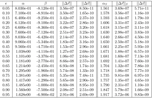
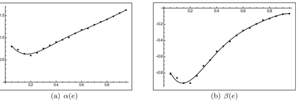
(11) Table 2: Optimal values α, β for each value of e in the bi-parametric family and optimal values αS in the Sundman family and errors in position and velocity.. e 0.05 0.10 0.15 0.20 0.25 0.30 0.35 0.40 0.45 0.50 0.55 0.60 0.65 0.70 0.75 0.80 0.85 0.90 0.95. α 8.030e-01 7.100e-01 6.400e-01 6.120e-01 6.600e-01 7.600e-01 8.030e-01 9.060e-01 9.560e-01 1.038e00 1.101e00 1.181e00 1.214e00 1.295e00 1.381e00 1.417e00 1.485e00 1.560e00 1.628e00. β -8.120e-01 -8.910e-01 -9.250e-01 -9.100e-01 -8.360e-01 -7.120e-01 -6.420e-01 -5.340e-01 -4.710e-01 -4.110e-01 -3.370e-01 -2.770e-01 -2.450e-01 -1.960e-01 -1.480e-01 -1.290e-01 -1.000e-01 -7.500e-02 -6.900e-02. ||∆#r || 3.56e-07 3.50e-07 3.42e-07 3.22e-07 4.48e-07 2.51e-07 2.14e-07 1.83e-07 1.53e-07 1.27e-07 1.06e-07 8.66e-08 6.93e-08 5.74e-08 5.35e-08 5.65e-08 8.60e-08 2.08e-07 2.91e-06. ||∆#v || 8.50e-11 1.65e-10 2.37e-10 2.86e-10 3.20e-10 3.23e-10 3.18e-10 3.16e-10 2.96e-10 2.68e-10 2.64e-10 2.57e-10 1.74e-10 1.33e-10 7.48e-11 2.90e-10 8.95e-10 2.51e-09 2.69e-09. αS 1.561 1.578 1.593 1.606 1.618 1.630 1.640 1.650 1.661 1.671 1.681 1.692 1.704 1.718 1.735 1.757 1.790 1.847 1.917. ||∆#r ||S 3.69e-07 3.56e-07 3.44e-07 3.31e-07 3.15e-07 2.98e-07 2.66e-07 2.50e-07 2.25e-07 1.88e-07 1.60e-07 1.41e-07 1.32e-07 1.06e-07 9.81e-08 1.35e-07 2.31e-07 5.79e-07 3.72e-06. ||∆#v || 5.71e-11 1.16e-10 1.79e-10 2.43e-10 3.11e-10 3.83e-10 4.50e-10 5.18e-10 5.93e-10 6.57e-10 7.13e-10 7.60e-10 7.86e-10 7.77e-10 6.97e-10 4.65e-10 1.10e-10 1.66e-09 9.83e-09. defined by αi = 0.01 · i, βj = 0.01 · j, for i, j = 0, . . . , 100, in order to get a first approximation and after that we use a gradient method to improve these values. The last columns of table 2 contain the optimal values in the case of the Sundman family of anomalies. These errors have been computed using a classic 4th order Runge-Kutta integrator with 1000 uniform steps. In this table, we can see that the value of α where the position errors reach their minimum depends on the eccentricity. The values of α and β where ||∆!r || reach its minimum can be connected to the eccentricity e by means of five order least square fitting-polynomials given by α(e) = −12.601e5 + 40.312e4 − 49.006e3 + 27.948e2 − 6.023e + 1.059. (45). β(e) = −16.579e5 + 50.911e4 − 59.682e3 + 31.794e2 − 5.961e − 0.569. (46). Figure 2 shows the dependence between the optimal values of the parameters α, β and the eccentricity e.. Figures 3, 4, 5 and 6 show the local integration errors in the coordinates (x, y) and the velocity (vx , vy ) in the orbital plane for a satellite moving in OXY plane and major semi-axis a = 118363.47 Km and eccentricity e = 0.7 for 11.

(12) (a) α(e). (b) β(e). Figure 2: Dependence of α and β parameters of e. several values of (α, β). These errors have been obtained by solving for each value of Ψα,β = i · h, where h = 2π/1000, the equation i · h = Ψα,β (g). From the value of g, we compute through the exact solution of the two-body problem the position and velocity vectors. These values are the initial conditions for the numerical integrator and we obtain the solution for the next step. To evaluate the exact local truncation errors, we compare the obtained value with the exact one calculated for the value of g given by (i + 1)h = Ψα (g).. (a) erx. (b) ery. (c) ervx. (d) ervy. Figure 3: Local integration errors distribution e = 0.7 for the Sundman anomaly α = 1.5, β=0. 12.

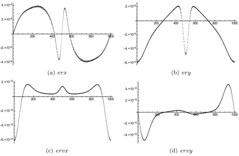
(13) (a) erx. (b) ery. (c) ervx. (d) ervy. Figure 4: Local integration errors distribution e = 0.7 for the optimal value in the Sundman family α = 1, 73, β = 0. (a) erx. (b) ery. (c) ervx. (d) ervy. Figure 5: Local integration errors distribution e = 0.7 for the elliptic anomaly α = 1.5, β = −0.5. 13.

(14) (a) erx. (b) ery. (c) ervx. (d) ervy. Figure 6: Distribution of the local integration errors e = 0.7 for the optimal anomaly in the bi-parametric family α = 1.295, β = −0.196. Table 3: Number of steps, n, to arrange a precision ||∆# r|| ∼ 10−6 Km using a RKF8(9) method combined with several anomalies. n ||∆!r || ||∆!v ||. M 138 1.1e-6 0.9e-9. g 91 1.1e-6 1.0e-9. τ∗ 86 1.0e-6 0.9e-9. f 75 1.0e-6 1.0e-9. f" 200 1.0e-6 0.8e-9. s∗ 113 1.0e-6 0.7e-9. w 119 1.0e-6 0.7e-9. Ψα,β 76 1.0e-6 1.3e-9. To evaluate the performance of integration methods with variable step size combined with the bi-parametric family of anomalies, we use a Runge-KuttaFehlberg RKF8(9) method with constant step size [5] with several anomalies of this family and we compute the number of steps necessary to obtain a position error ||∆!r || ∼ 10−6 Km. Table 3 contains these results and it has been obtained using a double precision arithmetic. Finally, to test the robustness of the method, we study the number of fix size steps necessary to obtain the satellite position with a precision of 10−4 Km after a hundred periods (469 days) in a perturbed problem, using a classical RungeKutta method of fourth order and a Runge-Kutta method of eighth order [5]. The perturbed problem is the motion of the satellite Heos II around the Earth including the main term due to the oblatness of the Earth. The disturbing potential U that appears in (1) is given [9], [12] by U = J2 GM. a2E P2 (sin φ), r3. 14. (47).

(15) Table 4: Number of steps to obtain the satellite position with ||∆# r|| < 10−4 Km after 100 revolutions using several anomalies. α β RK(4) RK(8). M 0 0 1102370 51193. g 1 0 388972 14387. τ∗ 1.5 0 276522 10987. f 2 0 251661 10378. f# 1 1 938892 34803. s∗ 0.5 -0.5 451743 18085. w 1.5 -0.5 264236 10481. Φα,β α(e) β(e) 231406 10286. where J2 = 0.0010920, aE = 6378.388 Km is the equatorial radius of the Earth, and φ the geocentric latitude of the satellite given by tan φ = √ 2z 2 and P2 (x) x +y. is the Legendre polynomial of ' second order P2 (x) = (3x2 − 1)/2. Obviously we have sin φ = x/r, and cos φ = x2 + y 2 r. ! = −∇U ! are given by: The perturbative forces derived of Φ $ 2% ) ∂U aE ( Φx = − = −3GM J2 P2 (sin(φ)) + sin φ2 cos φ x 5 ∂x r $ 2% ) ∂U aE ( Φy = − = −3GM J2 P2 (sin(φ)) + sin φ2 cos φ y 5 ∂y r $ 2% ) ∂U aE ( Φz = − = −3GM J2 P2 (sin(φ))z − sin φ cos φ3 r (48) 5 ∂z r Replacing (48) in (1), we have. Q dx = vx , dΨα,β n dy Q = vy , dΨα,β n Q dz = vz , dΨα,β n. Q x Q dvx = −GM + Φx 3 dΨα,β nr n dvy Q y Q = −GM + Φy dΨα,β n r3 n dvz Q z Q = −GM + Φz , dΨα,β n r3 n. (49). Table 4 shows the number of steps necessary to obtain a precision ||∆!r || < 10−4 Km after 100 revolutions using a classical Runge-Kutta method of fourth order and a Runge-Kutta of eighth order with constant step size [5] and several anomalies Ψα,β . 5. Concluding Remarks The bi-parametric family of anomalies includes for β = 0 the family of generalized Sundman anomalies, and for this reason, M , g, τ ∗ and f . This family also includes the regularized length of arc s∗ introduced by Brumberg, the elliptic anomaly w and the secondary anomaly f " . To study the optimal values of α and β in order to increase the performance of the numerical methods,. 15.

(16) a set of numerical experiments on the unperturbed two-body problem have been carried out. To test the robustness of the method, a perturbed problem has been studied. From its results, we conclude the goodness of the method. This family of anomalies is appropriate to develop the most common quantities of the two-body problem. It is very important to use these anomalies in analytical theories of the planetary motion. The difference between anomalies Ψα1 ,β1 and Ψα2 ,β2 is of second order in the eccentricity when α1 − β1 = α2 − β2 . This family is also appropriate to develop analytical planetary theories. In this sense, the main quantities that appear in the development of the second member of the planetary Lagrange equations have been obtained. To develop analytical theories it is convenient to use these developments combined with a Poisson series processor. Acknowledgements This research has been partially supported by Grant P1-1B2012-47 from Universidad Jaume I of Castellón and Grant AICO/2015/037 of Generalitat Valenciana. References [1] Brower, D., Clemence, G.M. 1965. Celestial Mechanics, Ed Academic Press, New York. [2] Brumberg, E.V. 1992. Length of arc as independent argument for highly eccentric orbits, Celestial Mechanics. 53 323–328. [3] Brumberg, E.V., Fufkushima, T. 1994. Expansions of Elliptic Motion based on Elliptic Functions Theory, Celestial Mechanics. 60, 69-89. [4] Deprit, A. 1979. A Note on Lagrange’s Inversion Formula,Celestial Mechanics. 20 325–327. [5] Fehlberg, E. 1968. Classical fifth-, sixth-, seventh-, and eighth-order Runge-Kutta formulas with stepsize control, Nasa Technical Report, Nasa TR R-287. [6] Hagihara, Y. 1970. Celestial Mechanics. vol 2., Ed MIT Press, Cambridge MA. [7] Janin, G. 1974. Accurate Computation of Highly Eccentric Satellite Orbits, Celestial Mechanics. 10, 451–467. [8] Janin, G., Bond, V. R. 1980. The elliptic anomaly, NASA Technical Memorandum 58228. [9] Levallois, J.J., Kovalevsky, J. 1971. Géodésie Générale Vol 4, Ed Eyrolles, Paris. 16.

(17) [10] López, J. A., Marco, F. J., Martı́nez, M. J. 2014. A Study about the Integration of the Elliptical Orbital Motion Based on a Special OneParametric Family of Anomalies. Abstract and Applied Analysis. Volume 2014, Article ID 162060 [11] López, J. A., Agost, V., Barreda, M. 2015. An improved algorithm to develop semi-analytical planetary theories using Sundman generalized variables. Journal of Computational and Applied Mathematics. 275, 403– 411. [12] Hofmann-Wellenhof, B., Moritz, H. 2005. Physical Geodesy, Ed SpringerWien, New York. [13] Nacozy, P. 1969. Hansen’s Method of Partial Anomalies: an Application. The Astronomical Journal. 74 544–550. [14] Nacozy, P. 1977. The intermediate anomaly. Celestial Mechanics. 16 309–313. [15] Tisserand, F. 1896. Traité de Mécanique Céleste, Ed Gauthier-Villars, Paris.. 17.

(18)