Radiofrequency architectures and technologies for software defined radio

(1)

UNIVERSIDAD POLITÉCNICA DE MADRID

E

SCUELA

T

ÉCNICA

S

UPERIOR DE

I

NGENIEROS DE

T

ELECOMUNICACIÓN

RADIOFREQUENCY ARCHITECTURES AND

TECHNOLOGIES FOR SOFTWARE DEFINED RADIO

T

ESIS

D

OCTORAL

Cristina de la Morena Álvarez-Palencia

Ingeniera de Telecomunicación

(2)

(3)

DEPARTAMENTO DE SEÑALES, SISTEMAS Y RADIOCOMUNICACIONES ESCUELA TÉCNICA SUPERIOR DE INGENIEROS DE TELECOMUNICACIÓN

UNIVERSIDAD POLITÉCNICA DE MADRID

RADIOFREQUENCY ARCHITECTURES AND

TECHNOLOGIES FOR SOFTWARE DEFINED RADIO

T

ESIS

D

OCTORAL

Autor:

Cristina de la Morena Álvarez-Palencia

Ingeniera de Telecomunicación

Director:

Mateo Burgos García

Catedrático del Departamento de Señales Sistemas y Radiocomunicaciones Universidad Politécnica de Madrid

(4)

(5)

T

ESIS

D

OCTORAL

RADIOFREQUENCY ARCHITECTURES AND TECHNOLOGIES FOR

SOFTWARE DEFINED RADIO

AUTOR:

Cristina de la Morena Álvarez-Palencia

DIRECTOR:

Mateo Burgos García

Tribunal nombrado por el Magfco. y Excmo. Sr. Rector de la Universidad Politécnica de Madrid, el día ___ de ____________ de 2012.

PRESIDENTE: Félix Pérez Martínez SECRETARIO: Manuel Sierra Castañer VOCAL: João Nuno Pimentel Silva Matos VOCAL: Eduardo Artal Latorre

VOCAL: Iván Alejandro Pérez Álvarez SUPLENTE: Blas Pablo Dorta Naranjo SUPLENTE: Íñigo Ederra Urzainqui

Realizado el acto de defensa y lectura de Tesis el día ___ de ____________ de 2012, en la E.T.S. de Ingenieros de Telecomunicación, Madrid.

Calificación:

EL PRESIDENTE LOS VOCALES

(6)

(7)

‘Dans les champs de l'observation le hasard

ne favorise que les esprits préparés’

‘In the fields of observation chance favors

only the prepared mind’

(8)

(9)

Acknowledgments

First of all, I would like to thank my supervisor, Professor Mateo Burgos

García, for giving me the opportunity to work under his direction. I really appreciate

all his support, guidance, vast knowledge, and helpful advices.

Special thanks to my collages and friends of the Grupo de Microondas y

Radar. We have shared many good times that I will never forget.

I am extremely grateful to Professor Bernard Huyart, who gave me the

opportunity to do a research stay in the Telecom ParisTech. I would like to thank him,

and the rest of the member of the Radiofrequencies and Microwave Group, for their

hospitality and kindness during my stay.

Last but no least, thanks to my family for the support they provided me

through my entire life. You are the most important thing to me.

This research was performed in the Microwave and Radar Group of the

Department of Signals, Systems, and Radiocommunications, Technical University of

Madrid. It was sponsored in part by the Spanish National Board of Scientific and

Technological Research (CICYT), under project contracts TEC2005-07010-C02-01,

TEC2008-02148, and TEC2011-28683-C02-01; and in part by INDRA Sistemas, under

TelMAX Project. Acknowledgments to the grant “IX Convocatoria de Ayudas del

Consejo Social, Universidad Politécnica de Madrid” for its financial support for the

(10)

(11)

Resumen

La red de seis puertos es una interesante arquitectura de radiofrecuencia que alberga múltiples posibilidades. Surgida en la década de los setenta como una alternativa a los analizadores de redes, en los últimos años se ha empleado en numerosas aplicaciones, tales como receptores homodinos, sistemas radar, detección de ángulos de llegada, UWB (Ultra-Wide-Band) o sistemas MIMO (Multiple Input Multiple Output). En la actualidad, se perfila como una de las mejores candidatas para implementar una Radio Definida por Software (SDR).

En esta tesis se estudia en profundidad esta prometedora arquitectura, describiendo sus fundamentos teóricos y realizando un estudio del estado del arte. Además, se presenta el diseño y desarrollo de un prototipo de receptor de seis puertos de banda ancha (0.3-6 GHz) para SDR, implementado en tecnología convencional. El sistema será caracterizado experimentalmente y validado para la demodulación de señales de radio frecuencia. El estudio y análisis de la arquitectura de seis puertos se completa con su comparación, teórica y experimental, con otras arquitecturas de RF, desde el punto de vista de su posible aplicación para SDR.

Varias son las aportaciones novedosas que se plantean en esta tesis. Dichas aportaciones se orientan en dos direcciones claras, que se corresponden con los actuales temas de interés en redes de seis puertos: desarrollo y optimización de técnicas de regeneración I-Q y algoritmos de calibración en tiempo real para redes multipuerto; y búsqueda de nuevas técnicas y tecnologías que contribuyan a la miniaturización de la arquitectura de seis puertos. En concreto, las contribuciones novedosas desarrolladas en esta tesis se resumen en:

• Introducción de un nuevo método de auto-calibración en tiempo real para redes multipuerto y aplicaciones de banda ancha, basado en canalización digital.

(12)

• Contribución a la miniaturización de receptores de seis puertos mediante el uso de la tecnología multicapa LTCC (Low Temperature Cofired Ceramic). Desarrollo de un receptor de seis puertos en tecnología LTCC de banda ancha (0.3-6 GHz) y tamaño reducido (30x30x1.25 mm).

(13)

Abstract

Six-port network is an interesting radiofrequency architecture with multiple possibilities. Since it was firstly introduced in the seventies as an alternative network analyzer, the six-port network has been used for many applications, such as homodyne receivers, radar systems, direction of arrival estimation, UWB (Ultra-Wide-Band), or MIMO (Multiple Input Multiple Output) systems. Currently, it is considered as a one of the best candidates to implement a Software Defined Radio (SDR).

This thesis comprises an exhaustive study of this promising architecture, where its fundamentals and the state-of-the-art are also included. In addition, the design and development of a SDR 0.3-6 GHz six-port receiver prototype is presented in this thesis, which is implemented in conventional technology. The system is experimentally characterized and validated for RF signal demodulation with good performance. The analysis of the six-port architecture is complemented by a theoretical and experimental comparison with other radiofrequency architectures suitable for SDR.

Some novel contributions are introduced in the present thesis. Such novelties are in the direction of the highly topical issues on six-port technique: development and optimization of real-time I-Q regeneration techniques for multiport networks; and search of new techniques and technologies to contribute to the miniaturization of the six-port architecture. In particular, the novel contributions of this thesis can be summarized as:

• Introduction of a new real-time auto-calibration method for multiport receivers, particularly suitable for broadband designs and high data rate applications.

• Introduction of a new direct baseband I-Q regeneration technique for five-port receivers.

(14)

(15)

Index of contents

1 INTRODUCTION ... 1

1.1 OVERVIEW OF SOFTWARE DEFINED RADIO IMPLEMENTATION ... 1

1.2 MOTIVATION AND SCOPE OF THE THESIS ... 4

1.3 THESIS ORGANIZATION ... 5

1.4 LIST OF PUBLICATIONS ... 6

2 STUDY OF RADIO FREQUENCY ARCHITECTURES FOR SOFTWARE DEFINED RADIO ... 9

2.1 INTRODUCTION ... 9

2.2 ZERO-IF ... 9

2.2.1 Fundamentals of zero-IF ... 9

2.2.2 Zero-IF in software radio applications ... 14

2.3 LOW-IF ... 14

2.3.1 Fundamentals of low-IF ... 14

2.3.2 Low-IF in software radio applications ... 15

2.4 SIX-PORT ARCHITECTURE ... 16

2.4.1 Fundamentals of six-port networks ... 16

2.4.1.1 Graphical interpretation ... 19

2.4.1.2 Design considerations on six-port junctions ... 22

2.4.2 Operation principle of six-port receivers ... 25

2.4.3 Advantages and drawbacks ... 31

2.4.4 Calibration methods and I-Q regeneration ... 33

2.4.4.1 Auto-calibration method based on training sequence ... 35

2.4.5 Six-port in software radio applications ... 36

2.5 SUMMARY ... 37

3 ... 39

(16)

3.3 SIX-PORT RECIEVER DESIGN AND SIMULATION ... 41

3.3.1 Six-port network ... 41

3.3.1.1 90-degree hybrid coupler ... 42

3.3.1.2 Power divider ... 49

3.3.1.3 Simulation of the six-port network response ... 50

3.3.2 Power detectors ... 53

3.3.2.1 Design considerations ... 53

3.3.2.2 .. ... 62

Wide video bandwidth and high dynamic range detector design 3.3.3 Complete six-port receiver ... 65

3.4 IMPLEMENTATION AND EXPERIMENTAL CHARACTERIZATION ... 70

3.4.1 90-degree hybrid coupler ... 70

3.4.2 Power divider ... 72

3.4.3 Six-port network ... 74

3.4.4 Complete six-port receiver ... 78

3.5 SIX-PORT DEMODULATION PERFORMANCE ... 80

3.5.1 Multi-mode and multi-band behaviour ... 81

3.5.2 Operation with low LO power levels ... 82

3.5.3 Comparison of multi-port demodulators ... 84

3.6 SUMMARY ... 86

4 COMPARISON BETWEEN SIX-PORT AND CONVENTIONAL RECEIVERS ... 87

4.2 ZERO-IF/LOW-IF RECEIVER PROTOTYPE ... 88

4.3 MEASUREMENT RESULTS ... 89

4.3.1 Performance comparison ... 90

4.3.2 Influence of the image frequency in low-IF ... 92

4.3.3 Influence of the LO power level ... 93

4.3.4 Conclusions ... 94

4.4 OPERATION OF SIX-PORT AS DUAL ZERO-IF/LOW-IF ARCHITECTURE ... 95

4.5 SUMMARY ... 98

5 I-Q REGENERATION TECHNIQUES FOR SIX/FIVE-PORT RECEIVERS ... 101

(17)

5.2 CHANNELIZED AUTO-CALIBRATION METHOD ... 101

5.2.1 Motivation... 101

5.2.2 Method description ... 102

5.2.3 Method validation ... 104

5.3 DIRECT BASEBAND I/Q REGENERATION METHOD FOR FIVE-PORT RECEIVERS ... 108

5.3.1 Motivation... 108

5.3.2 Method description ... 109

5.3.2.1 Orthogonality of the Regenerated I/Q Signals ... 112

5.3.2.2 Amplitude of the Regenerated I/Q Signals ... 114

5.3.2.3 DC-offset and IMD2 suppression ... 115

5.3.3 Method validation ... 117

5.3.3.1 Measured I/Q phase and amplitude imbalance ... 118

5.3.3.2 Measured DC-offset and IMD2 suppression ... 120

5.3.3.3 Demodulation results ... 123

5.4 SUMMARY ... 126

6 SIX-PORT RECEIVER IN LTCC TECHNOLOGY ... 127

6.2 ... 128

VALIDATION OF THE TECHNOLOGY: LTCC 90º HYBRID COUPLER DEVELOPMENT 6.3 LTCC SIX-PORT RECEIVER DESIGN AND SIMULATION ... 132

6.3.1 3-dB tandem coupler ... 132

6.3.2 Wilkinson power divider ... 135

6.3.3 LTCC six-port network ... 136

6.3.4 Complete LTCC six-port receiver... 137

6.4 IMPLEMENTATION AND EXPERIMENTAL CHARACTERIZATION ... 139

6.4.1 LTCC six-port network ... 140

6.4.2 Complete LTCC six-port receiver prototype ... 144

6.5 LTCC SIX-PORT DEMODULATION PERFORMANCE ... 146

6.6 SUMMARY ... 154

7 CONCLUSIONS AND PERSPECTIVE ... 155

(18)

(19)

Index of figures

Fig.1.1: Ideal SDR implementation. ... 2

Fig. 1.2: Comparison between (a) Conventional multimode radio, and (b) SDR. ... 3

Fig. 2.1: Block diagram of a zero-IF receiver. ... 10

Fig. 2.3: Block diagram of a low-IF receiver. ... 15

Fig. 2.4: Multiport network for the measurement of complex voltage ratios. ... 16

Fig. 2.5: Determination of Γ from the intersection of three circles. ... 21

Fig. 2.6: Determination of Γ from the intersection of two circles. ... 21

Fig. 2.7: Examples of six-port junction topologies. ... 23

Fig. 2.13: Block diagram of a six-port receiver ... 26

Fig. 2.14: Six-port receiver with analog I-Q regeneration. ... 34

Fig. 2.15: Six-port receiver with digital I-Q regeneration. ... 34

Fig. 2.16: Structure of a software defined radio six-port receiver. ... 37

Fig. 3.1: Block diagram of the proposed broadband SDR six-port receiver. ... 41

Fig. 3.2: Six-port network topology. ... 41

Fig. 3.3: Schematic of a tandem coupler. ... 42

Fig. 3.4: N-section symmetrical directional coupler. ... 43

Fig. 3.5: Broadside-coupled striplines (a) Overlap coupled striplines (b) Offset coupled striplines. ... 45

Fig. 3.6: Simulation schematic of the stripline 3dB tandem coupler. ... 47

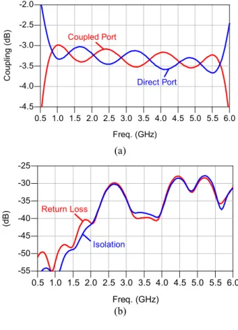
Fig. 3.7: Simulated amplitude response of the stripline 3 dB tandem coupler (circuital simulation): (a) Coupling, (b) Input return loss and isolation. ... 47

Fig. 3.8: Simulated phase difference between coupled and direct ports of the stripline 3 dB tandem coupler (circuital simulation). ... 48

Fig. 3.9: Layout of the 3dB tandem coupler generated from Momentum. ... 48

Fig. 3.10: Simulated amplitude response of the stripline 3 dB tandem coupler (EM simulation): (a) Coupling, (b) Input return loss and isolation. ... 49

Fig. 3.11: Simulated phase difference between coupled and direct ports of the stripline 3 dB tandem coupler (EM simulation)... 49

Fig. 3.12: Simulation schematic of the six-port network. ... 51

Fig. 3.13: Simulated attenuation from LO port to output ports of the six-port network. ... 51

Fig. 3.14: Simulated attenuation from RF port to output ports of the six-port network. ... 52

Fig. 3.15: Simulated input return loss and isolation of the six-port network. ... 52

Fig. 3.16: Simulated output return loss. ... 52

Fig. 3.17: Simulated phase shift from RF port to output ports of the six-port network, considering Port 3 as reference port. ... 53

Fig. 3.18: Simulated phase shift from LO port to output ports of the six-port network, considering Port 3 as reference port. ... 53

Fig. 3.19: Basic detector circuit. ... 54

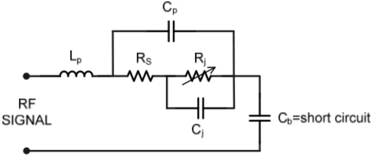
Fig. 3.20: Schottky diode equivalent circuit. ... 54

Fig. 3.21: Theoretical detector diode voltage sensitivity, HSMS-286B. ... 57

(20)

Fig. 3.23: Dynamic range improvement with bias, HP 5082-2751 detector (© Hewlett-Packard

App. Note 956-5 [124]). ... 59

Fig. 3.24: Detector equivalent circuit at the RF port. ... 60

Fig. 3.25: HSMS-286 diode input impedance. ... 60

Fig. 3.26: HSMS-286 diode input impedance with a 60 Ω shunt resistor. ... 60

Fig. 3.27: Detector equivalent circuit at the video port. ... 61

Fig. 3.28: Low-pass video coupling structure. ... 62

Fig. 3.29: Recommended application circuit for MAR8A+ implementation. ... 65

Fig. 3.30: Layout of the power detector. ... 65

Fig. 3.31: Schematic of the six-port receiver. ... 66

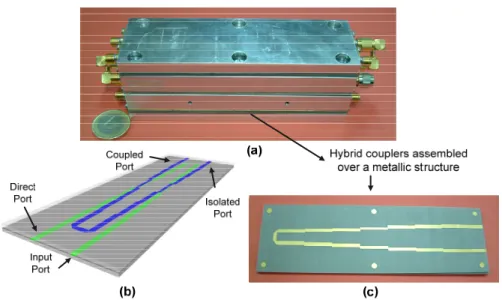
Fig. 3.32: Simulated output voltages of the six-port receiver: f =2595 MHz, f =2590 MHz, P =7.5 dBm, P =-40 dBm.OL RF ... 66LO RF Fig. 3.33: Simulated six-port receiver IF response (at output port 3): P =7.5 dBm, P =-40 dBm. ... 67LO RF Fig. 3.34: Simulated six-port receiver gain versus LO power (at output port 3): f - f =5 MHz, P =-40 dBm.RF ... 67LO RF Fig. 3.35: Simulated power of the even-order intermodulation product (at output port 3): P =-40 dBm, (a) f =780 MHz, (b) f =2595 MHz, (c) f =5786.5 MHz.LO LO LO ... 68RF Fig. 3.36: Simulated gain compression curve (at output port 3): f - f =5 MHz, P =7.5 dBm. ... 69LO RF LO Fig. 3.37: Photograph of the 3 dB tandem coupler in stripline technology. ... 70

Fig. 3.38: Assembly of the three tandem couplers (a) External appearance, (b) 3D view of the 3dB tandem coupler, (c) Top view of the 3dB tandem coupler. ... 71

Fig. 3.39: Simulated and measured coupling of the stripline 3 dB tandem coupler. ... 71

Fig. 3.40: Simulated and measured input return loss of the stripline 3 dB tandem coupler. ... 71

Fig. 3.41: Simulated and measured isolation of the stripline 3 dB tandem coupler... 72

Fig. 3.42: Simulated and measured phase difference between coupled and direct ports of the stripline 3 dB tandem coupler. ... 72

Fig. 3.43: Photograph of the LYNX 111.A0214 power divider. ... 73

Fig. 3.44: Measured insertion loss of the power divider... 73

Fig. 3.45: Measured return loss of the power divider. ... 73

Fig. 3.46: Measured phase imbalance of the power divider. ... 74

Fig. 3.47: Six-port network physical realization... 74

Fig. 3.48: Simulated and measured input return loss of the six-port network. ... 76

Fig. 3.49: Simulated and measured isolation of the six-port network. ... 76

Fig. 3.50: Measured attenuation from LO port to output ports of the six-port network. ... 77

Fig. 3.51: Measured attenuation from RF port to output ports of the six-port network. ... 77

Fig. 3.52: Simulated and measured phase response of the six-port network. ... 77

Fig. 3.53: Simulated and measured q -points of the six-port network (a) Magnitudes (b) Phases.i ... 78

Fig. 3.54: Six-port receiver prototype. ... 78

Fig. 3.55: Set-up of the six-port receiver test-bench. ... 81

Fig. 3.56: Constellation diagrams for 25 Mbps QPSK, P =–20 dBm (a) P =5 dBm (b) P =0 dBm (c) P =–10 dBm (d) P =–20 dBm.LO LO ... 83in LO LO Fig. 3.57: Theoretical BER versus EVM curves. ... 84

Fig. 4.1: Block diagram of the zero-IF/low-IF receiver... 88

Fig. 4.2: Zero-IF/low-IF receiver prototype. ... 89

Fig. 4.3: Set-up of the measurement test-bench. ... 90

Fig. 4.4: Measured EVM versus Pin: 2595 MHz, 30 Mbps 64-QAM, P =0dBm.LO ... 91

Fig. 4.5: Measured EVM versus Pin: 2595 MHz, 75 Mbps 64-QAM, P =0 dBm.LO ... 91

Fig. 4.6: Measured IF response of the zero-IF/low-IF receiver. ... 92

Fig. 4.7: Constellation diagrams: 2595 MHz, 25 Mbps QPSK, Pin=-25 dBm, P =0 dBm.LO ... 92

Fig. 4.8: Measured EVM versus P : 2595 MHz, 10 Mbps QPSK, Pin=-20 dBm.LO ... 94

(21)

Fig. 4.10: Constellation diagram obtained from the six-port receiver in low-IF operation mode.

... 96

Fig. 5.1: Frequency response of the family of N=4 filters. ... 103

Fig. 5.2: Scheme of the channelized auto-calibration method. ... 104

Fig. 5.3: Validation of the channelized auto-calibration method: 75 Mbps 64-QAM, 2.45 GHz (a) Measured EVM versus P (b) BER calculated from EVM.in ... 106

Fig. 5.4: Simulated BER versus SNR for a 420 Mbps 64-QAM signal and strong six-port frequency response variations. ... 107

Fig. 5.5: Structure of the analog I/Q regeneration circuit. ... 111

Fig. 5.6: Orthogonality degradation due to lack of symmetry. ... 114

Fig 5.7: Variation of 1/μI, 1/μQ, and tan(γ/2) with γ. ... 115

Fig. 5.8: Block diagram of the developed five-port receiver. ... 117

Fig. 5.9: Fabricated five-port circuit. ... 117

Fig. 5.10: Fabricated I/Q regeneration circuit. ... 117

Fig. 5.11: Measured amplitude and phase shift of the five-port circuit output signals (P =-35 dBm, P =0 dBm, LO Δf= 10 KHz), and simulated IQ phase difference. ... 119RF Fig. 5.12: Measured amplitude and phase of the received I/Q signals (P =-35 dBm, P =0 dBm, Δf= 10 KHz), and simulated I/Q phase difference. ... 119RF LO Fig. 5.13: Comparison between the measured phase shift of the five-port circuit output signals and the value of γ calculated from the measured IQ amplitudes. ... 119

Fig. 5.14: DC-offset suppression performance versus frequency, P =0 dBm.LO ... 121

Fig. 5.15: DC-offset suppression performance versus LO power, f=2.1 GHz. ... 121

Fig. 5.16: IMD2 suppression performance versus adjacent channel power, P (a) One interfering adjacent channel signal (b) Two interfering signals. ... 122adj Fig. 5.17: Set-up of the five-port receiver test bench. ... 123

Fig. 5.18: Structure of the transmitted data burst. ... 124

Fig. 5.19: Received constellations, P = -35 dBm, P =-3 dBm.RF LO ... 124

Fig. 5.20: Measured EVM versus frequency, P = -3 dBm, P =-35 dBm.LO RF ... 125

Fig. 5.21: Measured BER versus RF power of the QPSK modulated signal, f= 2.1 GHz, P =-3 dBm. ... 125LO Fig. 6.1: LTCC layer structure using DuPont-951 substrate. ... 128

Fig. 6.2: Cross section of the LTCC 8.34-dB coupler, DuPont-951 substrate. ... 129

Fig. 6.3: Top-view of the LTCC 3-dB tandem coupler, DuPont-951 substrate. ... 130

Fig. 6.4: Fabricated LTCC 3-dB tandem coupler, DuPont-951 substrate. ... 130

Fig. 6.5: Input return loss and isolation of the LTCC 3-dB tandem coupler, DuPont-951 substrate. ... 131

Fig. 6.6: Insertion loss of the LTCC 3-dB tandem coupler, DuPont-951 substrate. ... 131

Fig. 6.7: Amplitude and phase imbalances of the LTCC 3-dB tandem coupler, DuPont-951 substrate. ... 131

Fig. 6.8: LTCC layer structure using DuPont-943 substrate. ... 132

Fig. 6.9: Cross section of the LTCC 8.34-dB coupler, DuPont-943 substrate. ... 133

Fig. 6.10: Top-view of the LTCC 3-dB tandem coupler, DuPont-943 substrate. ... 134

Fig. 6.11: Simulated frequency response of the LTCC 3-dB tandem coupler, DuPont-943 substrate. ... 134

Fig. 6.12: Simulated amplitude and phase imbalances of the LTCC 3-dB tandem coupler, DuPont-943 substrate. ... 134

Fig. 6.13: Layout of the LTCC Wilkinson divider, DuPont-943 substrate. ... 135

Fig. 6.14: Simulated frequency response of the LTCC Wilkinson divider. ... 135

Fig. 6.15: Top-view of the LTCC six-port network. ... 136

Fig. 6.16: Distribution of the six-port receiver circuits in the 10 layer LTCC structure. ... 138

Fig. 6.17: Frequency response of the LFCV-45+ low-pass filter (a) without and (b) with a 33 pF capacitor. ... 138

Fig. 6.18: 3D-view of the LTCC six-port receiver (a) top (b) layers L1-L8 (c) bottom. ... 139

(22)

Fig. 6.21: Test-bench for the measurement of the six-port scattering parameters. ... 141 Fig. 6.22: Fabricated circuit test platform for the measurement of the six-port scattering

parameters. ... 141 Fig. 6.23: Detail of one output port with ground patches for probe positioning. ... 141 Fig. 6.24: Measured (solid line) and simulated (dashed line) input return loss and isolation. .. 142 Fig. 6.25: Measured (solid line) and simulated (dashed line) attenuations from the LO port. . 143 Fig. 6.26: Measured (solid line) and simulated (dashed line) attenuations from the RF port. .. 143 Fig. 6.27: Measured (solid line) and simulated (dashed line) magnitude of the q -points.i ... 143 Fig. 6.28: Measured (solid line) and simulated (dashed line) phase of the q -points.i ... 144 Fig. 6.29: Fabricated LTCC six-port receiver prototype. ... 144 Fig. 6.30: Measured IF response of the LTCC six-port receiver (at Port 3). ... 145 Fig. 6.31: Measured gain at the four output ports, f - f = 5 MHz.LO RF ... 145 Fig. 6.32: Measured phase difference between output ports (Port 3 as reference port), f - f = 5 MHz. ... 145LO RF Fig. 6.33: Set-up of the LTCC six-port receiver test bench. ... 147 Fig. 6.34: Test bench for the measurement of the LTCC six-port receiver. ... 147 Fig. 6.35: Received constellations: 15.625 Msymbol/s, P =0 dBm, P =-25 dBm, f=2.4 GHz.

... 148LO in Fig. 6.36: Measured EVM versus frequency: 75 Mbps 64-QAM, P =0 dBm, P =-20 dBm.LO in 148 Fig. 6.37: Measured EVM versus P : 75 Mbps 64-QAM, P =0 dBm, f=2.5 GHz.in LO ... 149 Fig. 6.38: Measured EVM versus P : 75 Mbps 64QAM, P =0 dBm, f=2.5 GHz,

Downsampling and Channelized AM, N=4.in ... 149LO Fig. 6.39: BER calculated from measured EVM: 75 Mbps 64-QAM, P =0 dBm, f=2.5 GHz

(23)

Index of tables

Table 1.1 Relation between objectives and publications of the thesis. ... 7 Table 3.1 Parameters of a seven-section 8.34 dB coupler: δ=0.35 dB, B=8.9622. ... 45 Table 3.2 MAR8A+amplifier electrical specifications at 25ºC and 36 mA. ... 64 Table 3.3 Simulated amplitude and phase relations of the six-port receiver output signals. ... 66 Table 3.4 Simulated six-port receiver characteristics, P =7.5 dBm.LO ... 69 Table 3.5 Measured six-port receiver characteristics, P =7.5 dBm.LO ... 79 Table 3.6 Measured EVM, P =0 dBm, P =-20 dBm.LO in ... 82 Table 3.7 Measured EVM versus P , 25 Mbps QPSK.LO ... 84 Table 3.8 Comparison of multi-port demodulation performances. ... 85 Table 4.1 Performance comparison of heterodyne, homodyne and multi-port techniques (with

(24)

List of abbreviations

3G: Third Generation Mobile Communications.

4G: Fourth Generation Mobile Communications.

ADC, A/D: Analog to Digital Converter.

ADS: Advanced Design Systems.

AGC: Automatic Gain Control.

ASIC: Application Specific Integrated Circuits.

AWGN: Additive White Gaussian Noise.

BER: Bit Error Rate.

BPSK: Binary Phase-Shift Keying.

CPU: Central Processing Unit.

DAC, D/A: Digital to Analog Converter.

DC: Direct Current.

DoA: Direction of Arrival.

DSP: Digital Signal Processor.

DUT: Device-Under-Test.

EVM: Error Vector Magnitude.

FIR: Finite Impulse Response.

FPGA: Field Programmable Gate Array.

GSM: Global System for Mobile communication.

IC: Integrated Circuit.

IF: Intermediate Frequency.

IMD2: Second-order intermodulation distortion.

IP3: Third Order Intermodulation Point.

JTRS: Joint Tactical Radio Service.

LNA: Low Noise Amplifier.

LTE: Long Term Evolution.

LO: Local Oscillator.

LTCC: Low Temperature Cofired Ceramic.

MEMS: MicroElectroMechanical Systems.

MIC: Microwave Integrated Circuit.

MIMO: Multiple Input Multiple Output.

MMIC: Monolithic Microwave Integrated Circuit.

P1dB: 1 dB Compression Point.

PCS: Personal Communications Service.

PSK: Phase-Shift Keying.

(25)

QoS: Quality of Service.

QPSK: Quadrature Phase-Shift Keying.

RF: Radiofrequency.

RFC: Radiofrequency Choke.

SDR: Software Defined Radio.

SIW: Substrate Integrated Waveguide.

SNR: Signal to Noise Ratio.

UMTS: Universal Mobile Telecommunications System.

UWB: Ulta-Wide-Band.

VSWR: Voltage Standing Wave Ratio.

VSG: Vector Signal Generator.

WiMAX: Worldwide Interoperability for Microwave Access.

WLAN: Wireless Local Area Network.

(26)

(27)

Chapter 1

1 I

NTRODUCTION

1.1 O

VERVIEW OF SOFTWARE DEFINED RADIO

IMPLEMENTATION

Information and telecommunication technologies are evolving towards a new concept of information society, where different communication standards are combined to form heterogeneous networks. This is precisely the concept of 4G or

Beyond 3G, since GSM and UMTS are combined with different access technologies, such us WLAN (Wireless Local Area Network) and WPAN (Wireless Personal Area Network). Users are demanding to communicate using different services, from wherever and whenever they want. However, the main problem derives from the incompatibility between the different standards and technologies.

(28)

Project 25 (APCO-P25) in EEUU [6] or Mesa Project in Europe [7]; satellite transceivers; etc.

The original idea of a SDR hardware implementation, conceived by Mitola in 1995 [8], consisted of placing the ADC (Analog to Digital Converter) just at the output of the antenna. Digital processing is performed by software, using DSPs (Digital Signal Processors), FPGAs (Field Programmable Gate Array) o ASICs (Application Specific Integrated Circuits). However, this implementation is currently impossible, due to the ADC limitations as for speed, dynamic range, jitter and power consumption [9]. For example, a 12 bit 11 Gsample/s ADC would be required to digitalize the frequency range from 800 MHz to 5.5 GHz, where all cellular communications and WLAN are located at present [10]. Obviously, such an ADC is currently impossible. But in the case it were possible, its power dissipation would be prohibitive. The state of the art is nowadays around 16 bit 130 MS/s A/D conversion for commercial Mitola’s type SDRs. In practice, the SDR hardware is composed of a reconfigurable baseband digital signal stage and a broadband radio frequency (RF) front-end.

Fig.1.1: Ideal SDR implementation.

Until now, conventional multi-band receivers have consisted of a different reception chain for each standard. This solution is not cost efficient, as it requires specific circuits for each standard, which increase the volume of the radio terminal. On the contrary, a SDR is composed of a single broadband reception stage. All channels are converted to digital domain with a high speed ADC, and channel selection is performed by software defined filters. However, the design of a universal general-purpose broadband RF front-end, with multi-mode and reconfiguration features, is not a simple matter. Furthermore, the difficulty increases if other aspects such as volume or cost are also taken into account.

Digital Processing DAC

(29)

- Frequency conversion - Channel selection

Fig. 1.2: Comparison between (a) Conventional multimode radio, and (b) SDR.

Superheterodyne architecture has been the classical configuration in radiocommunications, due to its selectivity and sensitivity characteristics. However, superheterodyne receivers are complex and expensive, as they require a large number of external components, including bulky RF filters for image frequency rejection. Another problem is the difficulty of changing system parameters such as bandwidth, because RF and IF signals are processed by fixed narrowband analog components, which make difficult to achieve a broadband system with multimode operation. Consequently, heterodyne architecture is not the best option when a SDR hardware implementation is addressed.

Two more suitable alternatives to implement a SDR are the direct frequency conversion architecture, also named homodyne or zero-IF, and the low-IF architecture [9]-[12]. Zero-IF and low-IF architectures have many advantages suitable for SDR, such as flexibility, reconfigurability, low-cost, simplicity, compact size, and high level of integration. However, these architectures have some limitations. In the case of zero-IF receivers, these limitations include DC-offset, 1/f noise, and second-order intermodulation distortion (IMD2). Regarding to the low-IF configuration, the image frequency continues being the main problem. Moreover, the trend towards high data rates services will require larger bandwidths, which become possible at high frequencies. Nevertheless, I-Q mod/demodulators cannot operate in very large frequency ranges, so the use of zero-IF and low-IF architectures is limited by these

(b)

ADC Ch 1

Analog Digital

- Frequency Conversion

- Channel selection

ADC

Analog Digital

ADC

Analog Digital

Ch 2

Ch 3 Software

ADC

Analog Digital Ch 1

Analog Filtering

Digital Filtering

(30)

Six-port network is an innovative and interesting architecture that is nowadays emerging as a promising alternative, as it does not use I-Q mixers for the frequency conversion [13]-[16]. The main characteristic of the six-port architecture is its extremely large bandwidth, which involves multi-band and multi-mode capabilities. Six-port networks can operate at very high frequencies [17]-[20], being a serious alternative for millimetre-wave frequencies and large relative-bandwidth applications. Furthermore, the six-port architecture can perform high data rates. A 200 Mbps data rate was estimated in 2008 [14], although recent publications have demonstrated the six-port capacity to demodulate 1.7 Gbps signals [21]. These and other advantages make this architecture to be considered a good candidate to implement a SDR.

However, apart from well known problems of direct conversion architectures, there are some issues in six-port networks that need intensive research. On one hand, six-port receivers require a calibration process to recover the original signal. Traditional physical calibration procedures, consisting on measuring the system using several external physical standards terminals, are impractical for a wireless receiver or a SDR, owing to their lack of dynamism and flexibility. Moreover, the performance of current real-time calibration methods will diminish when dealing with high-speed signals. On the other hand, the large dimensions of the passive six-port structure, especially for operating frequencies in the lower gigahertz region, could be prohibitive, for example, for mobile communication applications. In fact, the miniaturization of six-port receivers is the focus of current work.

1.2 M

OTIVATION AND SCOPE OF THE THESIS

The present thesis is mainly concerned with the investigation and optimization of RF architectures, in order to achieve a universal and flexible radio platform, with multi-mode and multi-band capabilities. In particular, this thesis focuses on the study of a very promising RF architecture, the six-port architecture, and its possible application to SDR.

Five main issues are addressed in this thesis:

(31)

multi-mode operation capabilities of the six-port receiver in the demodulation of RF signals.

2. Experimental comparison between six-port and conventional zero-IF and low-IF architectures.

3. Research and development of new and efficient multi-port calibration methods for digital IQ regeneration.

4. Investigation on new techniques for real-time analog I-Q regeneration.

5. Contribution to the miniaturization of six-port receivers.

The first two issues comprise an exhaustive study of the six-port architecture. The last three points are the main novel contributions of this thesis, as they are related to the topics that are currently having more intensive research in six-port networks.

1.3 T

HESIS ORGANIZATION

The thesis organization reflects the main directions of the research:

• Chapter 2 reviews the fundamentals of the three RF architectures with more possibilities to implement a SDR, i.e., zero-IF, low-IF, and six-port network.

• Chapter 3 addresses the design, development, and experimental characterization of an extremely large relative bandwidth six-port receiver.

• Chapter 4 presents an experimental comparison between the six-port receiver, and conventional zero-IF/low-IF receivers.

• Chapter 5 proposes two new I-Q regeneration techniques for six/five-port receivers. The first one is a real-time multi-port auto-calibration method, suitable for broadband applications and high-speed signals. The second technique is a direct baseband IQ recovery technique for five-port receivers, based on the use of a simple analog IQ regeneration circuit.

(32)

1.4 L

IST OF PUBLICATIONS

[TOEEJ 2008] C. de la Morena-Álvarez-Palencia, M. Burgos-García, F. Pérez-Martínez, “A Novel and Simple Maximum Available Gain Equalization Technique for Microwave Amplifiers,”

The Open Electrical and Electronic Engineering Journal, vol. 2, pp. 45-49, May 2008.

[URSI 2008] C. de la Morena-Álvarez-Palencia, A. Martín-López, M. Burgos-García, “Comparación entre arquitecturas de RF para Radio Definida por Software”, XXIII Simposium Nacional de la Unión Científica Internacional de Radio URSI 2008, Madrid, Spain, 22-24 Sept. 2008, pp. 149.

[SDRF 2009] C. de la Morena-Álvarez-Palencia, M. Burgos-García, “Reconfigurable radio technologies for professional wide band communications”, in European Reconfigurable Radio Technologies Workshop and Product Exposition, SDR forum, Madrid, Spain, 22-24 April 2009. Available: http://groups.winnforum.org/p/cm/ld/fid=69.

[URSI 2009] C. de la Morena Álvarez-Palencia, M. Burgos García, “Método de autocalibración canalizado para red de seis puertos”, in XXIV Simposium Nacional de la Unión Científica Internacional de Radio URSI 2009, Santander, Spain, 16-18 Sept. 2009, pp. 97.

[URSI 2010-1] C. de la Morena-Álvarez-Palencia, M. Burgos-García, J. Gismero-Menoyo, “Aplicación de la tecnología LTCC para la miniaturización de redes de seis puertos”, in XXV Simposium Nacional de la Unión Científica Internacional de Radio URSI 2010, Bilbao, Spain, 15-17 Sept. 2010, pp. 28.

[URSI 2010-2] D. Rodríguez-Aparicio, C. de la Morena-Álvarez-Palencia, M. Burgos-García, “Receptores zero-IF y low-IF para radio definida por software”, in XXV Simposium Nacional de la Unión Científica Internacional de Radio URSI 2010, Bilbao, Spain, 15-17 Sept. 2010, pp. 39.

[EuMC 2010] C. de la Morena-Álvarez-Palencia, M. Burgos-García, D. Rodríguez-Aparicio, “Three octave six-port network for a broadband software radio receiver”, in 40th European Microwave Conference, Paris, France, 28-30 Sept. 2010, pp. 1110-1113.

[ICCST 2010] C. de la Morena-Álvarez-Palencia, M. Burgos-García, D. Rodríguez-Aparicio, “Software Defined Radio technologies for emergency and professional wide band communications,” in IEEE Int. Carnahan Conf. Security Tech., San Jose, CA, 5-8 Oct. 2010, pp. 357-363.

[MILCOM 2010] C. de la Morena-Álvarez-Palencia, M. Burgos-García, “Broadband RF front-end based on a six-port network architecture for software defined radio,” in IEEE Military Communication Conference, San Jose, CA, 31 Oct. - 3 Nov. 2010, pp. 651-656.

[PIER 2011] C. de la Morena-Álvarez-Palencia, M. Burgos, "Four-octave six-port receiver and its calibration for boradband communications and software defined radios," Progress in Electromagnetics Research, vol. 116, pp. 1-21, April 2011.

[URSI 2011] C. de la Morena-Álvarez-Palencia, M. Burgos-García, “Comparación experimental de receptores para radio definida por software”, in XXVI Simposium Nacional de la Unión Científica Internacional de Radio URSI 2011, Leganés, Spain, 6-9 Sept. 2011, pp. 24.

[EuMC 2011] C. de la Morena-Álvarez-Palencia, M. Burgos, J. Gismero-Menoyo "Contribution of LTCC technology to the miniaturization of six-port networks," in 41th European Microwave Conference, Manchester, UK, 10-13 Oct. 2011, pp. 659-662.

(33)

[URSI 2012] C. de la Morena-Álvarez-Palencia, M. Burgos-García, J. Gismero-Menoyo, “Diseño y construcción de una red de seis puertos LTCC para un receptor radio software”, in XXVII Simposium Nacional de la Unión Científica Internacional de Radio URSI 2012, Elche, Spain, Sept. 2012, accepted for publication.

[MTT 2012-2] C. de la Morena-Álvarez-Palencia, M. Burgos-García, J. Gismero Menoyo, "Miniaturized 0.3-6 GHz LTCC six-port receiver for software defined radio,” IEEE Trans. Microwave Theory Tech., submitted for publication.

Table 1.1 Relation between objectives and publications of the thesis.

Chapter Objective Publications

2 Study and optimization of RF architectures for _{SDR implementation} [TOEEJ 2008] [URSI 2008] [SDRF 2009] 3 Development and validation of a broadband six-_{port receiver for SDR and high-speed applications} [MILCOM 2010] [EuMC 2010]

[PIER 2011] 4 Experimental comparison between six-port and _{conventional zero-IF and low-IF architectures} [URSI 2010-2] [ICCST 2010]

[URSI 2011] 5 Research and development of new and efficient multi-port calibration methods for digital IQ

regeneration

[URSI 2009] [PIER 2011] 5 Investigation on new techniques for real-time _{analog I-Q regeneration} [MTT 2012-1]

6 Miniaturization of six-port receivers: development _{of a compact broadband LTCC six-port receiver}

[EuMC 2011] [URSI 2010-1]

(34)

(35)

Chapter 2

2 S

TUDY OF RADIO FREQUENCY

ARCHITECTURES FOR SOFTWARE

DEFINED RADIO

2.1 I

NTRODUCTION

This chapter presents the study of the three RF architectures with more possibilities to implement a SDR: zero-IF, low-IF, and six-port network. Their fundamentals, as well as their main advantages and drawbacks, are described below. The state of the art in SDR applications is also presented for the three architectures.

2.2 Z

ERO

-IF

2.2.1 Fundamentals of zero-IF

(36)

heterodyne systems for several applications, especially SDR, where high level of integration and low-cost solutions are required [9]-[12].

The typical configuration of a zero-IF receiver is represented in Fig. 2.1. It is a simple structure, where the RF signal is directly down-converted to zero frequency by means of an I-Q demodulator and a local oscillator (LO) of the same frequency. Next, the I-Q components are low-pass filtered and converted to digital domain with an ADC.

Fig. 2.1: Block diagram of a zero-IF receiver.

The direct conversion architecture comprises clear benefits with respect to the heterodyne. On one hand, since IF is equal to zero, zero-IF receivers does not suffer from the image frequency problem. Therefore, large costly image rejection filters and IF circuits can be eliminated. On the other hand, main operations such as channel selection and amplification are baseband performed, where integration is much easier. Channel filtering can be performed either with a simple low-pass filter or in the digital domain, which raises the possibility of having a universal and multi-standard RF front-end. All these characteristics entail high level of integration, compact size, simplicity, low-power consumption, flexibility and system reconfigurability. Consequently, the direct-conversion architecture is very attractive for integrated and reconfigurable RF receivers. Nonetheless, it suffers from a number of problems that do not exist or are not as serious as in heterodyne receivers [26],[27]. This has been mainly the reason why homodyne receivers have not been as popular as heterodyne ones.

A. DC-offset

(37)

Furthermore, this offset voltage must be removed in the analog domain prior to sampling, otherwise, it can saturate the baseband amplifiers and ADCs [28]. There are two types of DC-offsets:

- Time-invariant DC-Offset. It is caused by the inherent DC value in the analog circuits and, therefore, it does not vary with time. Time-invariant offset is mainly generated in the LNA or the I-Q demodulator, due to drifts or mismatches in the analog circuits.

- Time variant DC-Offset. It consists in the phenomenon known as self-mixing. The self-mixing occurs when a strong, nearby signal mixes with itself, producing a DC component that appears as interference at the centre of the desired signal. This situation may take place in the cases shown in Fig. 2.2. Due to the isolation between the LO port and the inputs of the mixer and the LNA is not perfect, the LO signal is leaked to the inputs of the LNA and the mixer, producing a DC component at the output of the mixer -Fig. 2.2(a)-. The same effect happens when a strong interference leaks from the LNA or mixer input to the LO port and is multiplied by itself -Fig. 2.2(c)-. Moreover, DC-offset can be produced when the LO leakage signal in the LNA input is radiated from the antenna and reflected from external objects -Fig. 2.2(b)-. The amount of DC-offset coming from radiation is very difficult to predict, since its magnitude can change rapidly with the object movement, fading and multipath reception, etc.

(38)

signal energy around DC by choosing DC-free modulation schemes, such as BFSK (binary frequency shift keying) [29]. In such a case, a reasonable high-pass filtering can be performed, especially for wideband channels.

Most of the proposed alternatives for the DC-offset rejection consist in improving the mixer characteristics. This is useful not only for eliminating DC-offset, but also other typical zero-IF problems [30],[31]. Other methods are based on the use of either analogical [32],[33] or digital DC-offset cancelling loops, although the combination of both [34] is more effective. In fact, the habitual procedure consists in combining both analogical and digital methods. Therefore, it is usual to apply digital compensation, equalization or calibration techniques, together with some of the methods presented above [35]-[37].

B. I-Q imbalances

(39)

pulses in the other channel, degrading the signal-to-noise ratio if the I and Q data streams are uncorrelated. Consequently, I-Q demodulator becomes a key element in direct conversion receivers. Nevertheless, I-Q mismatch is much less problematic in direct conversion schemes than in image-reject architectures.

C. Flicker noise

Flicker noise is characterized by presenting a power spectral density inversely proportional to the frequency. That is the reason why it is also called 1/f noise. Since 1/f noise is predominant at low frequencies, the downconverted signal is considerable affected by flicker noise, as it is located around zero frequency. Flicker noise, together with DC-offset, is a main issue in direct conversion receivers [38]. Most of the methods used for DC-offset cancelation are also useful for eliminating the 1/f noise components, especially those using mixers for low noise and high linearity [30]-[31],[39]-[40].

D. Even-order intermodulation distortion

While typical RF receivers only suffer from odd-order intermodulation effects, the even-order distortion is also a problem in direct conversion receivers, especially second-order intermodulation distortion (IMD2) [41],[42]. For example, let us consider the situation where two strong interferers, cos(2πf1t) and cos(2πf2t), separated

in frequency an amount f2-f1=Δ less than the bandwidth of interest, are exposed to a

second-order nonlinear behavior. In such a case, undesirable baseband spectral components are generated. These include a DC component and a baseband beat located at Δ Hz, within the downconversion band, which degrade the reception of the wanted signal. The solution leads to implement linear mixers, with higher rejection to second-order intermodulation, as well as the use of calibration techniques [42]-[45].

E. LO leakage

(40)

2.2.2 Zero-IF in software radio applications

The problems commented above have been the reason why homodyne receivers have not been as popular as heterodyne ones. Nevertheless, as different solutions have appeared in the last years, more and more zero-IF receivers for multimode applications have been proposed [46]-[47]. Moreover, new circuits and algorithmic techniques, along with higher levels of integration, have made zero-IF an acceptable choice for multi-standard reception. At present, SDRs based on the zero-IF architecture are capable of covering all cellular and WLAN communications, that is, up to 6GHz [48]-[50]. In fact, practically all commercially available SDRs for wireless communications are based on the zero-IF architecture. For example, Epic Solutions’

Matchstiq [51] is a 2.2”x4.6”x0.9” reconfigurable zero-IF transceiver with CPU/FPGA processing, which covers the 0.3-3.8 GHz frequency range and supports up to 28 MHz channel bandwidths (4500 $). The FUNcube Dongle [52] (64-1700 MHz, 80 kHz quadrature sampling rate, 86x23x14 mm) uses an E4000 CMOS multiband tuner, which is based on a zero-IF architecture indeed. Lime Microsystems commercializes the LMS6002 [53], a fully integrated (9x9 mm) 0.375-4 GHz zero-IF transceiver with programmable channel bandwidth from 1.5 to 28 MHz.

The challenge for zero-IF SDRs is currently focused on the exploration of higher frequencies, such us millimetre waves, as the trend towards high data rate services demands. The limit is determined by the I-Q mod/demodulator devices, thereby many efforts are being done in order to reach such a challenge [54]. Moreover, the development of broandband tunable RF filters, and wide band amplifiers is also having intensive research [TOEEJ 2008].

2.3 L

OW

-IF

2.3.1 Fundamentals of low-IF

(41)

Fig. 2.3: Block diagram of a low-IF receiver.

Low-IF receiver combines the advantages of zero-IF and heterodyne receivers. On one hand, low-IF has zero-IF advantages such as low-cost, compact size, reconfigurability, and high level of integration. On the other hand, as IF is not located around DC, there are no DC-offset and flicker noise problems. However, the main drawback of the low-IF architecture is the image frequency. As the image frequency is located very closed to RF signal, no RF filters for image rejection can be used. Typical image suppression techniques consist in using image rejection architectures, such as Hartley [56] or Weaver [57]. However, I-Q imbalances cause interference that can not be removed in later stages and so directly decrease the image-reject capabilities of the front-end. For example, a relative voltage gain mismatch of 5% and a phase imbalance of 5º lead to an image rejection ratio (IRR) approximately equal to 26 dB. The fact is that, in practice, these architectures can hardly achieve an IRR above 40 dB. Digital signal processing can also be applied to eliminate the image components [58]-[60]. However, the key point is that very strict I-Q balance requirements are demanded for low-IF receivers, making difficult its implementation, especially for broadband applications. Furthermore, a low-IF receiver demands the double IF bandwidth compared with a zero-IF receiver, making the I-Q imbalance problem worse.

2.3.2 Low-IF in software radio applications

(42)

a low-IF architecture [61]-[62]. Moreover, it is also usual to find SDRs which use both low-IF and zero-IF schemes [63]-[65].

2.4 S

IX

-

PORT ARCHITECTURE

2.4.1 Fundamentals of six-port networks

The origin of the six-port network dates from the seventies, when it was introduced by Engen and Hoer to measure complex voltage ratios, as an alternative network analyzer [66]-[69]. According to the classical six-port theory, the reflection coefficient of a DUT (device-under-test) connected to one of its ports can be determined by means of a certain set of remote independent observations, when an excitation is introduced into one of the other ports [70],[71].

1

a

2

b

2

a

n

a

n

b

3

b

3

a

-1

n

a b_n_-1

1

b

Fig. 2.4: Multiport network for the measurement of complex voltage ratios.

Let us consider the n-port network of Fig. 2.4, where the reflection coefficient of the DUT wants to be determined. Incident and reflected waves can be

related by means of the scattering parameters as follows:

2 2

= /

Γ a b

n j

a S b n

k k jk

j 1,2,...,

1

= =

∑

=

(2-1)

where S_jk are known complex parameters, and a_j,b_j are, respectively, the complex

envelopes of the incident and reflected waves, which are unknown parameters. Therefore, there are 2n unknowns.

(43)

= · = 3,..., i i i

a Γ b i n (2-2)

by joining the expressions (2-1) and (2-2), and after algebraic manipulations, the next system of equations is obtained:

⎥ ⎦ ⎤ ⎢ ⎣ ⎡ ⎥ ⎥ ⎥ ⎦ ⎤ ⎢ ⎢ ⎢ ⎣ ⎡ = ⎥ ⎥ ⎥ ⎦ ⎤ ⎢ ⎢ ⎢ ⎣ ⎡ 2 2 3 3 3 · ... ... ... b a b b n n

n α β

β α

(2-3)

i

α and β_i are known complex constants, since they depend on S_jk

2/b2

and . A

system of n-2 equations and two unknowns, and , is obtained. Then two

observations, for example b₃ and , are sufficient to resolve the system of equations

for and , obtaining the reflection coefficient of the DUT . Take into

account that any pair

i

Γ

2

a b₂

4

b

2

a b₂ Γ =a

j

a and/or bj could have been specified as unknowns in (2-3),

instead of and . The main problem is that, in practice, it is not an easy matter to

measure the reflected waves , being simpler to measure their powers:

2

a b2

i b 2 1 = 2 i i

P b (2-4)

Substituting (2-3) into (2-4), the next expression for the power of is

obtained: i b

(

) (

)

(

)

2 *

2 2 2 2 2 2

2 2 2 2 _* _* _* _*

2 2 2 2 2 2

1 1 = + = + · + 2 2 1 = + + + 2

i i i i i i i

i i i i i i

P αa βb αa βb αa βb

α a β b α β a b α βa b

=

(2-5)

(2-5) is linear with a₂2, b₂2, and . Hence, it is possible to determine

and with four power readings, that is, n=6. These four powers and the

remaining two ports (DUT and local oscillator, LO) are the reason for the name “six-port”. The system of equations results in:

* 2 2

a b * 2 2

a b

2

(44)

⎥ ⎥ ⎥ ⎥ ⎥ ⎦ ⎤ ⎢ ⎢ ⎢ ⎢ ⎢ ⎣ ⎡ ⋅ = ⎥ ⎥ ⎥ ⎥ ⎥ ⎦ ⎤ ⎢ ⎢ ⎢ ⎢ ⎢ ⎣ ⎡ ⋅ ⎥ ⎥ ⎥ ⎥ ⎥ ⎦ ⎤ ⎢ ⎢ ⎢ ⎢ ⎢ ⎣ ⎡ = ⎥ ⎥ ⎥ ⎥ ⎦ ⎤ ⎢ ⎢ ⎢ ⎢ ⎣ ⎡ 2 * 2 * 2 2 2 2 2 2 2 * 2 * 2 2 2 2 2 2 6 * 6 * 6 6 2 6 2 6 5 * 5 * 5 5 2 5 2 5 4 * 4 * 4 4 2 4 2 4 3 * 3 * 3 3 2 3 2 3 6 5 4 3 2 1 b a b a b a M b a b a b a P P P P β α β α β α β α β α β α β α β α β α β α β α β α (2-6)

which can be solved if M is not a singular matrix, i.e., |M|≠ 0. Under this condition, the previous system is solved as follows:

⎥ ⎥ ⎥ ⎥ ⎦ ⎤ ⎢ ⎢ ⎢ ⎢ ⎣ ⎡ ⋅ = ⎥ ⎥ ⎥ ⎥ ⎥ ⎦ ⎤ ⎢ ⎢ ⎢ ⎢ ⎢ ⎣ ⎡ − 6 5 4 3 1 2 * 2 * 2 2 2 2 2 2 P P P P M b a b a b a (2-7)

where the complex constant parameters α_i and β_i have to be determined in advance

using an appropriate calibration technique. It is worth to pointing out that determining

2 2

a , b₂2, *_and _{does not provide the absolute phases of and . In effect,}

as is the complex conjugate of , both quantities lead to the determination of

2 2

a b * 2 2

a b a2 b2

* 2 2

a b *

2

a b2

2·b2

a , and arg

( )

a₂ - arg

( )

b₂ . With the help of a₂2 andb₂2, a₂ and b₂ can be calculated, butonce again we have the term arg

( )

a₂ - arg

( )

b₂ . In practice, the habitual procedure consists of defining all the phases with respect to one reference port. In any

case, the reflection coefficient Γ =a₂/b₂ is completely defined by a₂ , b₂ and

( )

a2 arg

( )

b2

arg - .

Moreover, a₂2, b₂2, *_and _{are related to each other by} 2 2

a b * 2 2

a b

2 2 _* _*

2 · 2 = 2 2· 2 2

a b a b a b (2-8)

Consequently, (2-5) can be rewritten as:

(

2 2 2 2

)

(

)

2 2 2 2 2

1

= + + · · · cos arg( ) - arg( ) + arg( ) - arg( )

2

i i i i i i i

P α a β b α β a b α β a b₂ (2-9)

(45)

function leads to two solutions for arg

( )

a₂ - arg

( )

b2 . Thus, the problem does not have

unique solution for a five-port network, which means less accuracy in the measurements and a more complicated calibration process for the determination of

and

i

α

i

β [72]. This affirmation results evident from the six-port graphical interpretation,

which will be presented below.

2.4.1.1 Graphical interpretation

It was shown that the power readings at the four detection ports of a six-port junction are:

{

}

2

2 2

1

= + = 3,4,5,

2

i i i

P αa βb i 6

ber 3, that is, and

(2-10)

When operating as an alternative network analyzer, the six-port reflectometer is usually designed in such a way that the response of one of the power detectors is proportional to |b2|2 [69]. It responds to a double purpose. On one hand, |b2|

represents directly one of the measurements of interests. On the other hand, monitoring |b2| is useful to correct possible power instabilities in the signal source, and

to ensure that the power levels at the output ports are maintained at some optimum values as the frequency is varied. Then, the six-port comprises a reference port. The port chosen for this role will be num α₃= 0

2 2

3= 3 · 2

P β b (2-11)

Thus, the powers of the remaining ports can be normalized by P3, leading to:

{

}

2

2 2

3 ₃ ₂

+

= =

·

i i

i αa βb

P

, i

P _β _b 4,5,6 (2-12)

Defining the so-called qi-points as [69]:

= - i i

i

β

q

α (2-13)

(46)

{

}

2

2 3

= - = 4,5

i

i i

α

P

Γ q , i

P _β ,6 (2-14)

The above expression represents three circles, whose centres are the qi-points,

and their radius are

{

}

3 3

= - = i = 4,5,6

i i

i

β

P

R Γ q , i

P α (2-15)

Then, Γ is given by the intersection of these three circles, as it can be seen in Fig. 2.5. Six-port reflectometers are thus characterized by their qi-points, which can be

directly calculated from the six-port scattering parameters:

1 22 1 2 21 =

-i i

i i

s q

s s s s (2-16)

The determination of Γ could be also done by the intersection of only two circles, which would correspond to a five-port network. It is worth highlighting that in such a case, represented in Fig. 2.6, there are two possible solutions for Γ, as the two circles intersect in a pair of points. When the DUT is a passive device, Γ falls within the unit circle. Therefore, if one of the two points is outside the unit circle, which is the situation in Fig. 2.6, it is possible to choose between the two solutions.

In practice, due to measurement errors and detector noises, the circles do not intersect in the right position. In the case of six-port networks, their intersection will comprise a triangular area, where Γ will be included. As for five-port junctions, obviously, less accuracy in the determination of Γ is expected. In fact, there is a high sensitivity to errors in the direction perpendicular to the line between q3 and q5, being

less in the parallel direction. In particular, if Γ is located around the perimeter of the unit circle, one can assume a considerable variation in the sensitivity to errors.

Six-port reflectometers can be also designed without the requirement of α3=0.

(47)

q6

Γ

q5 q4

|Γ-q6|

UNIT CIRCLE |Γ-q4|

|Γ-q5|

Fig. 2.5: Determination of Γ from the intersection of three circles.

Fig. 2.6: Determination of Γ from the intersection of two circles.

{

}

2 2 2

2 2

2 2 2

3 _{3 2} _{3 2} ₃ ₃

+

-=

+

-i i i i

i αa βb α Γ q

P

= , i

P _α_a _β_b _α _Γ _q = 4,5,6 (2-17)

The above equation is a circle equation indeed, so it can alternatively be written as follows:

{

}

2

2₌ _- _{= 4,5,6}

i i

(48)

The centre and radius of the circles are now: 2 ₂ * 3 3 2 -= -i i i i i i k

q μ q q Q k μ (2-19)

(

)

2 2 3 ₄ 3 2 2 3 2 -= -i i i i

i

i i

qμ μ

k q q R q μ k (2-20) being 3 = i i P k

P , and

3 = i i α μ α .

Notice that the central position of the circles, Qi, are now functions not only of

the six-port junction, but also of the power readings in the Γ plane. Moreover, these power readings are directly related to the load connected to the measuring port 2. Then, a six-port design with α3=0 is advantageous in order to eliminate the dependence

of the Qi-points on the power readings and, therefore, on the load.

2.4.1.2 Design considerations on six-port junctions

The design criterion of a six-port junction consists of achieving a good distribution of the qi-points in the Γ plane [69]. By simple inspection of Fig. 2.5, it is

evident that an ill-conditioned numerical situation results if |qi| is either too large or too

small. Thus, based on symmetrical configurations, the optimal position of the qi

-points should be located at the vertices of an equilateral triangle whose centre is at the origin. This calls for |q4|=|q5|=|q6|, while the relative phase separations between qi are

120º. The optimum choice of |qi| may be expected to lie in the range 0.5-1.5.

Nevertheless, the six-port network can provide good results even when the ratios of the magnitudes of qi are greater than 4, and their arguments differ an amount smaller than

25º [73],[74]. In practice, most of the six-port junctions are quasi-optimal design approaches. In general, the closer the magnitudes of qi, and the larger the differences

between the arguments of qi, the better will be the performance of the circuit.

(49)

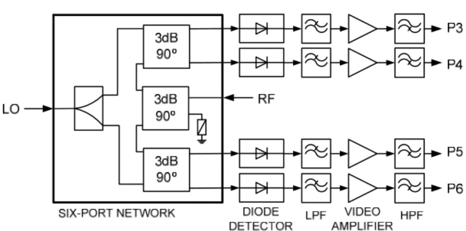
implementation of a broadband optimal six-port circuit can not be accomplished. In effect, a 120º phase shift is achieved with narrowband circuits, such as symmetrical five-port rings [75]—Fig. 2.7 (b)— or phase shifters based on delay lines [76]-[77]. On the contrary, a quasi-optimal six-port design can be realized using only 3dB hybrids and/or power dividers, making ultra-broadband six-port designs feasible [78]-[79]. For example, the topology represented in Fig. 2.7 (c) is the typical six-port configuration [13],[16], where a broadband 90º phase shift can be achieved using three 3dB hybrids and one Wilkinson divider.

A variety of different technologies have been used for six-port implementation. Several six-port network implementations are presented in Fig. 2.8-Fig. 2.12. Along with conventional MIC (Microwave Integrated Circuits) technology, six-port networks can be implemented, for example, in SIW (Substrate Integrated Waveguide), MMIC (Monolithic Microwave Integrated Circuit), or multilayer substrate technologies.

(50)

(51)