Research related to vibrations from high speed railway traffic

RESEARCH RELATED TO VIBRATIONS FROM HIGH SPEED

RAILWAY TRAFFIC

JOSE M. GOICOLEA Comp. Mech. Group, Escuela Ing. de Caminos Tech. Univ. of Madrid Madrid - Spain

FELIPE GABALDÓN Comp. Mech. Group, Escuela Ing. de Caminos Tech. Univ. of Madrid Madrid - Spain

ABSTRACT

We discuss here recent results from several research programmes related to dynamic aspects and vibrations induced by high speed railway traffic, developed at the computational mechanics group, within the “Escuela de Ingenieros de Caminos” of the Technical University of Madrid. The first part of this work concerns the dynamic response of railway bridges and structures under high speed traffic. The study of vertical dynamic effects in bridges has lead recently to improved understanding and practical design concepts, embodied in the new engineering codes [1,2,3,4,5]. Some special and seldom considered features of the dynamic response are also discussed. In the second part we present some results for lateral dynamic effects. These have not been so widely studied as the vertical vibrations, however they may pose significant problems for bridges. Finally, in the third part we discuss recent results of ongoing research for the mechanical response of slab track and ballast track, focusing on the vertical vibration of the track and the associated dynamic traffic loads.

1. VERTICAL VIBRATION OF BRIDGES

1.1 Moving loads and interaction models

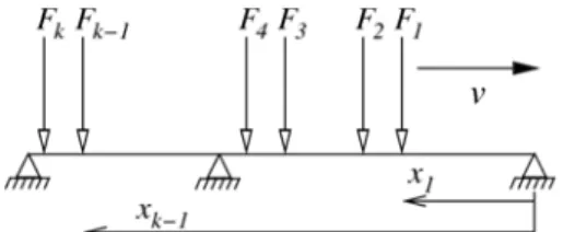
Dynamic analysis may be carried out by direct application of moving loads, with each axle represented by a load Fi travelling at the train speed v (Figure 1). This may be performed by

the degrees of freedom to be integrated. A direct integration of the complete model is also possible, albeit very costly for large three-dimensional models.

Figure 1. Load model for a train of moving loads

In principle, each response magnitude to be checked should be evaluated independently in the dynamic analysis; however, this may not be practical for engineering calculations. A common simplification is to perform a dynamic calculation to compute a single overall impact factor measuring a characteristic magnitude E, such as the displacement at mid-span. This factor is

later assumed to apply for all the response magnitudes to be checked. In such way, a real

impact factor may be computed from the dynamic analysis [1]:

Φ

_real

=

E

_dyn,real

/

E

_sta,LM71. Although not totally rigorous, the dynamic analysis of a characteristic displacement (e.g. vertical displacement at mid-span) is often taken as representative of dynamic effects for other design variables such as section forces, stresses, etc. This assumption will be discussed below with more detail in section 1.4.

It is important to consider also ELS dynamic limits [3], [9] (maximum acceleration, rotations and deflections, etc.), which are often the most critical design issues in practice. Accelerations must be independently obtained in the dynamic analysis. In the example shown in Figure 2 both maximum displacements and accelerations are obtained independently and checked against their nominal (LM71) or limit values respectively.

1.2 Dynamic analysis with bridge-train interaction

The consideration of the vibration of the vehicles with respect to the bridge deck allows for a more realistic representation of the dynamic overall behaviour. The train is no longer represented by moving loads of fixed value, but rather by masses, bodies and springs which represent wheels, bogies and coaches. A general model for a conventional coach on two bogies should include the stiffness and damping (Kp, cp) of the primary suspension of each axle, the

secondary suspension of bogies (Ks, cs), the unsprung mass of wheels (Mw), the bogies (Mb, Jb),

and the vehicle body (M, J). Further details of these models are described in [10], incorporating

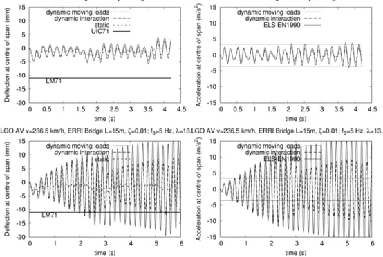
Figure 2. Calculations for simply supported bridge from ERRI D214 (2002) (L=15 m, f0=5

Hz, ρ=15000 kg/m, δLM71=11 mm), with TALGO AV2 train, for non-resonant (360

km/h, top) and resonant (236.5 km/h, bottom) speeds, considering dynamic analysis with moving loads and with train-bridge interaction. Note that the response at the higher speed (360 km/h) is considerably smaller than for the critical speed of 236.5 km/h. The graphs at left show displacements, comparing with the quasi-static response of the real train and the LM71 model, and those at right accelerations, compared with the limit of 3.5 m/s2 proposed in [3]

An application of dynamic calculations using moving loads and simplified interaction models is shown in Figure 2. A considerable reduction of vibration is obtained in short span bridges under resonance by using interaction models. This may be explained considering that part of the energy from the vibration is be transmitted from the bridge to the vehicles. However, only a modest reduction is obtained for non-resonant speeds. Furthermore, in longer spans or in continuous deck bridges the advantage gained by employing interaction models will generally be very small. This is exemplified in Figure 3, showing results of sweeps of dynamic calculations for three bridges of different spans. As a consequence it is not generally considered necessary to perform dynamic analysis with interaction for design purposes.

1.3 Short span bridges

different bridges, from short to moderate lengths (20 m, 30 m and 40 m). The maximum response obtained for the short length bridge is many times larger that the other. The physical reason is that for bridges longer than coach length at any given time several axles or bogies will be on the bridge with different phases, thus cancelling effects and impeding a clear resonance. We also remark that for lower speeds in all three cases the response is approximately 2.5 times lower than that of the much heavier nominal train LM71. Resonance increases this response by a factor of 5, thus surpassing by a factor of 2 the LM71 response.

Figure 3. Normalised envelope of dynamic effects (displacement) for ICE2 high-speed train between 120 and 420 km/h on simply supported bridges of different spans (L=20 m, f0=4 Hz, ρ=20000 kg/m, δLM71=11.79 mm, L=30 m, f0=3 Hz, ρ=25000 kg/m,

δLM71=15.07 mm and L=40 m, f0=3 Hz, ρ=30000 kg/m, δLM71=11.81 mm). Dashed

lines represent analysis with moving loads, solid lines with symbols models with interaction. Damping is ζ=2% in all cases

1.4 Evaluation of displacements and other dynamic response magnitudes

In some situations specific dynamic response magnitudes other than displacements are required directly from the analysis model. This situation arises when a more precise evaluation is required than what would be obtained by using an overall factor Φreal (as defined in section 1.1)

computed from a displacement response. Here we would like to call the attention to the fact that the model to be employed, for instance the number of modes considered in the integration, need not be the same for all cases.

To illustrate this we develop a model problem, a sudden step load P at the centre of a simply

⎪ ⎪ ⎪ ⎭ ⎪ ⎪ ⎪ ⎬ ⎫ ⎥ ⎥ ⎥ ⎥ ⎥ ⎥ ⎦ ⎤ ⎢ ⎢ ⎢ ⎢ ⎢ ⎢ ⎣ ⎡ − ⎟ ⎟ ⎠ ⎞ ⎜ ⎜ ⎝ ⎛ ⎟ ⎠ ⎞ ⎜ ⎝ ⎛ ₋ − − ⎟ ⎠ ⎞ ⎜ ⎝ ⎛ ₋ − − ⎪⎩ ⎪ ⎨ ⎧ − = ⎟ ⎠ ⎞ ⎜ ⎝ ⎛

∑

∑

∞ = − − − − − − − ∞ = − − 1 4 2 1 2 1 2 2 1 2 1 2 2 1 2 1 2 1 4 4 3 1 2 1 2 ) 1 2 ( 1 sin 1 1 cos ) 1 2 ( 1 2 , 2 n t n n n n n n n n n e n t t t n EI PL t L ω ς ς ω ς ς ς ω π δ (1) ⎪ ⎪ ⎪ ⎭ ⎪ ⎪ ⎪ ⎬ ⎫ ⎥ ⎥ ⎥ ⎥ ⎥ ⎥ ⎦ ⎤ ⎢ ⎢ ⎢ ⎢ ⎢ ⎢ ⎣ ⎡ − ⎟ ⎟ ⎠ ⎞ ⎜ ⎜ ⎝ ⎛ ⎟ ⎠ ⎞ ⎜ ⎝ ⎛ ₋ − − ⎟ ⎠ ⎞ ⎜ ⎝ ⎛ ₋ − ⎪⎩ ⎪ ⎨ ⎧ − ⎥ ⎦ ⎤ ⎢ ⎣ ⎡ − − = ⎟ ⎠ ⎞ ⎜ ⎝ ⎛

∑

∑

∞ = − − − − − − − ∞ = − − 1 2 2 1 2 1 2 2 1 2 1 2 2 1 2 1 2 1 2 2 1 2 1 2 ) 1 2 ( 1 sin 1 1 cos ) 1 2 ( 1 2 , 2 n t n n n n n n n n n e n t t t n PL t L M ω ς ς ω ς ς ς ω π (2)

In the steady-state, taking the limit for

t

→

∞

we recover the static values as expected,

EI PL EI PL n EI PL t L

n 96 48

2 ) 1 2 ( 1 2 , 2 3 4 4 3 1 4 4 3 = = ⎥ ⎦ ⎤ ⎢ ⎣ ⎡ − = ⎟ ⎠ ⎞ ⎜ ⎝ ⎛ _→∞

_∑

∞ = π π π δ (3) 4 8 2 ) 1 2 ( 1 2 , 2 2 2 1 2 2 PL PL n PL t L M n = − = ⎥ ⎥ ⎦ ⎤ ⎢ ⎢ ⎣ ⎡ − − = ⎟ ⎠ ⎞ ⎜ ⎝ ⎛ _→∞

_∑

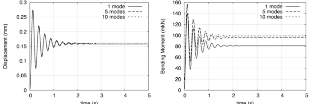
∞ = π π π (4)

Figure 4. Response of simply supported bridge (L=20 m, f0=4 Hz, ρ=20000 kg/m) under step

load P=20 kN, with damping ζ=10%. Results for displacement and for bending

moment at centre of span as a function of the number of modes considered [11]

1.5 Dynamic effects on continuous deck bridges

We discuss next some recent results related to evaluation of dynamic effects for continuous beam bridges. It is known [12] that in comparative terms the vibration effects in such bridges from moving railway traffic are generally significantly smaller than for simply supported (isostatic) bridges. However, there has been some concern recently regarding the effects for continuous bridges of spans between 50 and 60 m. The application of dynamic factors

ϕ

'

well established in railway applications and proposed in [13] in fact would predict amplifications reaching 1.20, for heavy freight trains at conventional speeds circa 100 km/h. Recently, in the context of the drafting of the new European Technical Specifications for interoperability for railway infrastructure [5] the point was brought up, as this effect would require the incorporation of a factor

α

≥

1

.

21

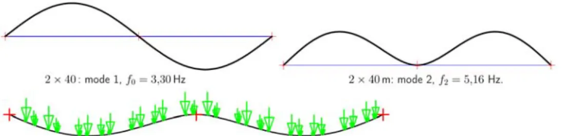
to be applied to the LM71 and SW/0 load models. In particular, this coefficient would be required for the case of loads corresponding to E5 line category. These vehicles include 25 tons of mass per axle corresponding to a mass per unit length of 8.8 ton/m.

Figure 5. In the top row, the two first modes of vibration of a 2-span continuous railway bridge, span lengths of 40 m. It is the second mode which causes the greatest part of the section forces at the bridge over the central support, i.e. negative moments. Below is presented a snapshot during the simulation for a train of E5 wagons, showing that it is in fact predominantly this second mode which is being excited under the traffic loads

We show in Figure 6 some representative results of this work. It may be seen that, even for the worst case scenarios of bridges and train speeds, the dynamic effects due to vibration remain moderate. In particular, these effects are covered sufficiently by a factor of

α

=

1

.

1

, which is the value included in the final text of the TSI [5].

Figure 6. Results for the quasi-static (green) and dynamic (red) responses of 2 span continuous bridges, under traffic of E5 wagons at 100 km/h. The left graph shows the displacements at the centre of one span, the right graph the (negative) moments at the support section. This case corresponds to one of the most critical cases, for a bridge with 60 m spans and the E5 train travelling at 60 km/h, in which case the second mode is excited producing the largest moments at the support. It may be seen that even in this worst case scenario the dynamic effects are small

1.6 Dynamic uplift

We discuss finally some results and proposals for evaluating dynamic uplift effects. Some of these results have been the base of code provisions in the code IAPF-2007 [1].

limiting case is the minimum vertical loads simultaneously with maximum horizontal loads (centrifugal and wind mainly). This aspect is not addressed directly in [2], where an unloaded train is proposed for these scenarios. The results shown here summarise those described with

greater detail in [15].

As a result of interpreting the dynamic response as oscillations around a quasi-static state it is possible to obtain bounds for maxima and minima, computed from the said static response and the amplitude of oscillation. Figure 7 shows the vertical reaction in a pier between two (simply supported) spans in a real bridge (Tajo river), computed for two different models with the Eurostar train. Details of the structure and of analysis model may be found in [16]. The first case corresponds to a dynamic model, for a speed of 225 km/h which was shown to produce resonance, with a moving load model. The second case is a quasi-static low-speed model (20 km/h), whose results are superposed on to the dynamic case.

The results show that the dynamic vibration may be interpreted as a dynamic effect

±Δ

E

_din

which is superposed on the quasi-static value,

E

_sta. The maximum dynamic effects obtained would be

E

max

=

S

sta

+

Δ

E

dyn, whereas the minima would result

E

max

=

S

sta

-

Δ

E

dyn. The time

instant in the figure for which the level

E

_min shown ceases to be a lower bound corresponds to a moment at which the train has already exited the first span, which then remains in free vibration. The minimum dynamic effects correspond to unloadings, that is upward reactions. Although these are significant, they would not effectively produce a lifting of the deck from the pier which would prescribe an anchorage, due to the permanent self-weight loads. However, their consideration may be necessary for some design features such as those governed by horizontal loads.

Figure 7. Time history of vertical reactions at a pier of Tajo river viaduct (simply supported spans), for Eurostar train at a speed of v=225 km/h (resonant speed)

Figure 8. Time history of bending moment at the centre of the first span of the continuous deck viaduct over Cabra river, for Eurostar train at a speed of v=420 km/h (speed for maximum dynamic effects)

2. LATERAL DYNAMIC VIBRATION IN RAILWAY BRIDGES DUE TO TRAFFIC

2.1 Motivation: experimental evidence and ERRI D181

three aspects: the magnitude of lateral forces, minimum lateral stiffness of bridge decks and minimum value of frequency of lateral vibration of bridge decks. In summary, the recommendations incorporated into the codes prescribe lateral axle loads of 100 kN, and a minimum frequency of lateral vibration of deck spans of 1.2 Hz, in order to avoid resonance with railway vehicles.

A number of viaducts in the new Spanish high speed railway lines have a low lateral stiffness for the global modes of deformation, which in principle could cause some concern for the lateral stability and ride comfort. They do not correspond to the cases studied by ERRI D181 [17], as the decks are closed sections and possess a great lateral stiffness. However, lateral deformations at the rail centerline alignment are produced by eccentric loads on double track decks, which originate both bending of the piers and torsion of the deck. The effect of lateral bending of the deck itself is generally negligible, due to the higher bending stiffness of a full section slab or box.

As a representative example we consider the “Arroyo las Piedras” viaduct (Figure 9), with several piers taller than 93 m and a total continuous length of the deck of 1209 m, within the new HSR line Córdoba-Málaga. This deck is a mixed steel-concrete structure with steel girders and concrete slab, with spans of 63,5 m. The design is due to Millanes [18], and the viaduct has been put in operation with the opening of the line to commercial passenger traffic in dec 2007 showing no important dynamic lateral vibration. In Figure 10 the first two modes of vibration are pictured, showing a frequency of 0.29 Hz for the first mode, considerably below the above mentioned requirement for lateral frequency.

Figure 10. Modes of vibration 1 (f_1=0.29 Hz) and 2 (f_2=0.37Hz) for viaduct “Arroyo las Piedras”. The lower modes correspond to lateral movement of the deck from bending of the piers

A similar response in terms of lateral stiffness and vibration modes has been obtained in many other viaducts of similar characteristics in the new HSR lines. However, it must be considered that the modes of deformation involved are global modes of bending due to bending of the piers, with a wavelength of several spans and much longer than one railway car. The ERRI D181 report, Eurocode EN1990-A1 and IAPF requirements refer literally to “the first natural frequency of lateral vibration of a span”, which should be interpreted as the deformation of the deck assuming the supports at the ends of the span rigid.

In order to attain resonance in the vehicles for global lateral deformation modes of long wavelengths it would be necessary for virtually all the vehicles, i.e. the complete train, to oscillate laterally in unison, which seems unlikely. More probably the lateral movements excited in each vehicle will be produced at random phases and cancel each out globally, at least to a certain extent. Finally, we also remark that the main concern in this case refers to the vibration of the vehicles and not to the limit states of the bridge which are generally not reached.

The motivation of this work is to assess the lateral deformation of long, laterally flexible viaducts under traffic loads of HS trains and the associated vibration in the vehicles. The calculations include the main aspects which cause lateral vibration of the vehicles: 1) lateral displacements in the plane of the track due to deformation of the bridge under eccentric vertical traffic loads; 2) track alignment irregularities; 3) hunting oscillations from conicity of wheel-rail contact.

The analyses were carried out in two successive calculations. Firstly, the traffic loads were run for different trains at several speeds, and histories of displacements at the track axis were obtained. These histories allowed the generation of virtual paths for the axles of a given bogie.

The methodology outlined above defines the coupling between vehicle and bridge in a weak manner, as the ensuing dynamic lateral load histories are not fed back into the structural calculations. It was checked that the deformations of the bridge were small for the lateral loads experienced, and consequently the results could be taken as a valid approximation. Following a summary of the research is outlined, more details may be found in [19], [20].

2.2 Vehicle models

Three vehicle types were considered in this work: passenger vehicles representative respectively of AVE S-103 train (Siemens ICE-3) and AVE S-100 train (Alstom), as well as the UIC freight wagon as defined in [17].

The AVE S103 vehicles are conventional cars with two bogies in each. The AVE S-100

vehicles are articulated, sharing bogies between adjacent cars. Each bogie has two axles,

connected to the bogie by the primary suspension; in turn, the bogies are connected to the car body by the secondary suspension. Finally, the UIC freight wagon has only one suspension system connecting the car body directly to the wheelsets. The mechanical parameters of the vehicle models are detailed in [19], [20]. In the case of the articulated AVE S-100 train the model needed to represent not only the central vehicle but an approximation of the adjacent ones connected to the end bogies as well, with half of the mass of each one. This was essential to model properly the bogies and restrain the yaw rotation. Due to this fact the vehicle model includes primary and secondary longitudinal suspensions also. These data are not included in the other vehicle models because their influence is not relevant.

In the models, in terms of boundary conditions, only the reference points at the centre of each wheelset was constrained, in which rotations about the three axes and the longitudinal and vertical motions were restrained. Only lateral (z) movement is allowed at these points, to which

Figure 11. AVE S-100 finite element vehicle model developed in ABAQUS [21]. Connection points in a bogie of the vehicle and referential axis of the suspensions or connector elements. Reference points for mass and inertia moments are marked in blue

2.3 Actions considered

For the dynamic analysis, three different actions responsible for lateral vibration of railway vehicles, when crossing a bridge, were considered: 1) lateral displacements in the plane of the track due to deformation of the bridge under eccentric vertical traffic loads, 2) track alignment irregularities and 3) hunting oscillations from conicity of wheel-rail contact.

2.3.1Bridge lateral displacements

Lateral displacements in railway bridges from traffic loads result from eccentric vertical loads in bridges with double track deck. Two effects from these loads must be considered (Figure 12): bending of supporting piers and torsion of the deck.

θ δ1

Support Midspan

δ1 δ2

Figure 12. Representation of lateral displacement of the deck due to bending of the piers δ1

(support section) and deck torsion δ2 (midspan)

In the following, for considering these displacements the concept termed here virtual path will

be used. This is defined as a function

u

z

(

x

)

representing the displacement of the track (lateral

in this case,

u

z) at a moving point which follows the train on its motion along the bridge. Note

represented as a displacement time-history curve, by a simple change of variables. This change represents the equivalence between time and train position,

v

=

x

⋅

t

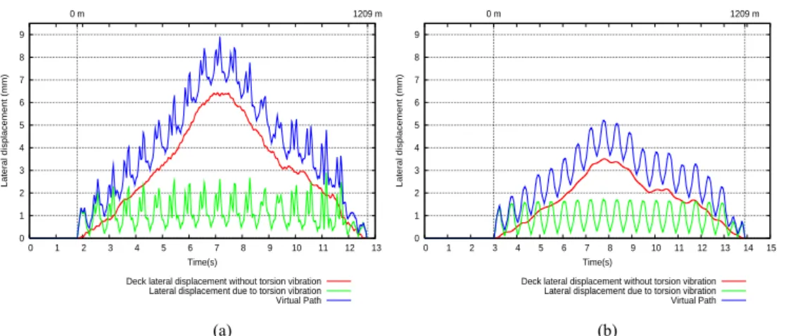
with appropriate choice of zero value of coordinates. Both scales are represented in the virtual paths of Figure 13.

Figure 13. Representation of virtual paths due to the passage of the AVE S-100 and AVE S-103 trains: (a) virtual path for an axle of the train S-100 located 200.15 m from the head of the train, at 400 km/h; (b) virtual path for an axle of the S-103 train located 336.06 m from the first axle of the train, at 400 km/h

A virtual path was computed given for each axle/bogie of the train. In Figure 7 the virtual path for the selected axles of the S-100 and S-103 trains are shown, when crossing the “Arroyo las Piedras” viaduct at v = 400 km/h. Each virtual path was obtained at points every 10 cm along the deck. In the figures, the red line represents bending lateral displacements δ1 and the green

line torsional displacements δ2. In blue the total lateral displacement from the two effects is

shown. It may be clearly seen that the bending of piers produces a long wave motion (with wavelength equal to the length of the bridge), whereas the torsional deformations produce a shorter wave motion (with wavelength equal to the span). Furthermore, for some velocities dynamic amplification from vibration of the bridge is obtained. The bogies or axles have been selected to represent worst cases for torsional lateral deformations δ2, which proved to be the

actions with a greater effect on vehicle lateral motion.

2.3.2Track alignment irregularities

Railway track irregularities are normally due to wear and tear, clearances, subsidence, inadequate maintenance, etc. The rail irregularities are assumed to be stationary random and ergodic processes in space, with zero mean values. They are characterized by their respective one sided power spectral density functions,

Φ

V_,A

(

Ω

)

, in which

Ω

is the spatial frequency or

wave number. In the present study, the power spectral density functions based on measurements performed in German railway tracks are adopted, following the empirical formula for alignment irregularities proposed by [22], as used by [23]:

0 1 2 3 4 5 6 7 8 9

0 1 2 3 4 5 6 7 8 9 10 11 12 13

1209 m 0 m

Lateral displacement (mm)

Time(s)

Deck lateral displacement without torsion vibration Lateral displacement due to torsion vibration Virtual Path

0 1 2 3 4 5 6 7 8 9

0 1 2 3 4 5 6 7 8 9 10 11 12 13 14 15

1209 m 0 m

Lateral displacement (mm)

Time(s)

Deck lateral displacement without torsion vibration Lateral displacement due to torsion vibration Virtual Path

,

)

)(

(

)

(

_{2 2 2 2}

2 ,

Ω

+

Ω

Ω

+

Ω

Ω

=

Ω

Φ

c r c A

V

A

(5)

where A,

Ω

c = 0.0206 rad/m and

Ω

r = 0.8246 rad/m define the actual data. Sample rail

irregularity profiles were generated numerically. For this study, the value of A was assumed to

be equal to 0.2119×10-6 _{rad·m which provided sample profiles with similar root mean-square}

values (standard deviation) to the alert limits proposed in [24]. Typical profiles generated are shown in Figure 14.

Figure 14. Track alignment irregularities profiles for the different intervals of of wavelengths considered, as defined in [24]. (a) D1, (b) D2, (3) D3 and (4) D3x (with lower track quality). The dashed lines indicate the alert limits for standard deviation

2.3.3Action from lateral wheel-rail interface

Due to the conicity of the geometry of rail-wheel contact, an oscillatory periodic lateral motion may develop. In this case we report the calculations based on the simplest model, which results in the most conservative evaluation. This is the case of the well known oscillatory Klingel motion (see e.g. [25]). We are currently developing more realistic models including wheel-rail

-10 -5 0 5 10

0 200 400 600 800 1000 1200 1400

Irregularties (mm)

Track length (m)

Track alignment irregularities with wavelengths between 3 and 25

σlimit -10 -5 0 5 10

0 200 400 600 800 1000 1200 1400

Irregularties (mm)

Track length (m)

Track alignment irregularities with wavelengths between 25 and 70

σlimit -10 -5 0 5 10

0 200 400 600 800 1000 1200 1400

Irregularties (mm)

Track length (m)

Track alignment irregularities with wavelengths between 70 and 120

σlimit -10 -5 0 5 10

0 200 400 600 800 1000 1200 1400

Irregularties (mm)

Track length (m)

Track alignment irregularities with wavelengths between 70 and 120 with low quality

σlimit

(a) (b)

interface following linearised Kalker’s theory. The values adopted for the lateral movement (3 mm) have been taken considering the maximum nominal values proposed in the European TSI [4].

2.4 Results

The calculations were carried out with the actions defined above, by direct integration in time in the ABAQUS finite element program. As previously mentioned, the actions were applied to the models in the centre of the wheelsets of each bogie, with appropriately defined different actions on each bogie or axle of a given vehicle. This consideration is important in order to excite the yaw motion (rotation around vertical y axis) of the car body.

From the analysis of the transfer functions of the vehicle models, it may be foreseen that the maximum dynamic response will be obtained for actions with higher frequencies of excitation. Thus, it was expected a higher vehicle dynamic response due to the combination of actions with irregularities profiles of short wavelength. This was what effectively happened in all the cases except for the UIC freight wagon.

The results for the S-100 train vehicle model are presented in Figure 15, in which the lateral accelerations in the centre of gravity of the car body and the lateral reaction forces in the wheelsets of one bogie are presented. Is possible to see that the accelerations are not high, being below the value of 1 m/s2_{, and the lateral reaction forces on the wheelsets are generally}

below 100 kN with some isolated peaks of around 200 kN. The results for the S-103 vehicle model are shown in Figure 16. These are clearly lower than those obtained for the S-100 vehicle model. Accelerations are always below 0.5 m/ s2_.

-1 -0.5 0 0.5 1

0 2 4 6 8 10 12

Accelerations (m/s

2)

Time (s)

Accelerations in the centre of gravity of the AVE train car body

Path+irreg+Klingel Path+irreg Path

-200 -100 0 100 200

0 2 4 6 8 10 12

Forces (kN)

Time (s)

Reaction forces on the wheelsets of each bogie

Path+irreg+Klingel Path+irreg Path

Figure 16. Lateral accelerations in the centre of gravity of the car body and lateral reaction forces in the wheelsets of one bogie of the S-103 vehicle model, considering for the combination of action a profile of irregularities with wavelengths within 3 m and 25 m and a speed of 400 km/h. In blue the response to only the virtual path (deformation of viaduct), the green curve includes also track irregularities and in red the previous plus hunting motion

3. VIBRATIONS OF BALLAST AND SLAB TRACK

3.1 Motivation and Scope of Project

The main functions of the railway track are to provide guidance in a secure and economic way for the trains, and to support the loads transmitted to the ground or underlying structures. The ballast track provides a traditional technology, which has been experienced for many years. Recently more innovative technologies of slab track without ballast have been introduced and are being operated successfully, the main exponents being the Japan Shinkansen track and the German lines (Figure 17). Among the main advantages of the slab track are the much reduced maintenance, allowing a more efficient operation, and the greater geometric quality of the track. The main drawback is the greater investment cost, as the track requires very strict tolerances regarding deformation of the foundation.

Figure 17. Rheda200 slab track

-1 -0.5 0 0.5 1

0 2 4 6 8 10 12

Accelerations (m/s

2)

Time (s)

Accelerations in the centre of gravity of the ICE2 train car body

Path+irreg+lazo Path+irreg Path

-200 -100 0 100 200

0 2 4 6 8 10 12

Forces (kN)

Time (s)

Reaction forces on the wheelsets of each bogie

With the objective of assessing several aspects of the comparative mechanical behaviour of the slab and ballast tracks, we are currently developing a research project funded by the Spanish government, including the following objectives undertaken by different teams: 1) Structural behaviour of the track and its foundation, including geotechnical requirements, requirements for degradation and damage of the slab, and dynamic loads transmitted to the track (Technical University of Madrid); 2) Behaviour and requirements regarding interaction between the slab track and structures (Fundación de Caminos de Hierro); 3) Interaction between rail and vehicles (CEIT of S. Sebastián and University of Basque Country); and 4) Transmission of noise vibrations through the foundation (Engineering faculty of University of Seville). A partial report with progress details of project is [26].

In the following we present some considerations regarding the models employed and some preliminary results. We shall focus exclusively on the dynamic loads resulting from vibrations in the structures and the vehicles, in consonance with the scope of this paper. The objective in this field is to determine for the track scenarios considered the dynamic loads transmitted by railway traffic, concentrating on high speed passenger traffic. The focus is on the vertical loads, neglecting in a first approximation the lateral forces.

3.2 Models for vehicles and tracks

The analysis is being carried out using two-dimensional models, which include the vehicle and the track, coupled with a Hertzian contact vertical interface.

We first show the simplified models for vehicles which are being considered for evaluation of dynamic vertical loads on track structures, see Figure 18. A number of simplifying assumptions are included, taking into account that depending on the scenario often the full three-dimensional multibody dynamic models are not required for vertical dynamics. Taking advantage of these simplifications, a complete set of sweeps regarding velocities, vehicle types, track configurations may be considered.

Regarding models for the track, the two basic configurations for ballast track and slab track are shown schematically in Figure 19. The parameters for the ballast track correspond to the high performance track laid by Spanish railway infrastructure manager ADIF, in the new high speed lines such as Madrid-Barcelona and Córdoba-Málaga, intended for speeds of up to 350 km/h. Some basic characteristics regarding frequency response for the track are presented in Figure 20.

Figure 19. Models employed for ballast track and slab track (Rheda2000)

Figure 20. frequency response functions of track models (ballast at left, slab track at right) and most significant modes of ballast track: left sleepers on ballast, centre rail on pads, right pin-pin

Figure 21. Validation results of dynamic results of models on track. On the left the three vehicle models (half axle with 1 DOF in red, quarter bogie with 2 DOF in blue, eighth vehicle with 3 DOF in black dashed line) are compared. It is seen that the simplest 1 DOF model fails to show adequately the response, which is virtually identical between the 2 DOF and 3 DOF models. On the right such a model is employed for the two successive axles in a bogie, showing virtually no interaction and a purely local effect

Due to lack of space we do not present here the full details of mechanical parameters of the models, which may be seen in [26]. The vehicle models are representative of current high speed trains in Spain (AVE S-100, S-101, S-102 and S-103).

3.3 Track irregularities

The vertical contact interface between wheel and rail has been modelled with a Hertz contact model. A key aspect for the evaluation of the dynamic loads is the consideration of track elevation irregularities, defined as random variables with the appropriate amplitude and wavelengths. A similar PSD function as defined above in section 2.3.2 for track alignment irregularities has been employed here for elevation. The more significant cases with regards to vertical dynamic loads are the very short wavelengths (λ∈[0.05,3]m) and the short

wavelengths (λ∈[3,25]m), D1 interval. The amplitude was defined as the maximum that

would trigger alarm limits as defined in [24], and consequently be limited by maintenance action. A representation of these profiles is shown in Figure 22.

3.4 Results for ballast track

As representative results, we present some preliminary calculations for ballast track, and the AVE S-103 vehicles (ICE3 train). In Figure 23 we first show the results for dynamic models on a perfect track, i.e. with no irregularities. The interaction effect for dynamic loads is here only that of the vertical deformation of the rail considered as a beam on elastic supports. It is seen that the dynamic increment is small, with a maximum of around 3%. On the contrary, the irregularities with wavelengths in the D1 range show approximately 25% dynamic increase. The results for very short irregularities (

λ

∈

[

0

.

05

,

3

]

m

) are shown in Figure 24, it may be seen that the dynamic effect is significantly larger, reaching 60%.

Figure 23. Amplification of vertical displacements at rail supports for perfect rail (left) and for distributed irregularities with short wavelength (at right, D1, λ∈[3,25]m)

Figure 24. Amplification of vertical displacements at rail supports for distributed irregularities with very short wavelength (λ∈[0.05,3]m).

4. CONCLUDING REMARKS

The lateral vibrations on structures induced by traffic or other actiosn is a topic which deserves more research attention, some relevant situations are not yet sufficiently understood.

Finally, an important question is the comparative dynamic behaviour of ballast and slab track and the consequences for durability and life cycle.

ACKNLOWLEDGEMENTS

The financial support of project PEIT2006 with ref PT-2006-024-19CCPM, Ministerio de Fomento, as well as other support in research projects from the same ministry is acknowledged. The support both financial and technical of the Fundación de Caminos de Hierro and Mr Jorge Nasarre is very much appreciated. Finally, most of this work has been developed by researchers in our group (J. Domínguez, J.A. Navarro, R. Dias, C. Vale) who deserve the merit for the results.

REFERENCES

[1] MFOM 2007. IAPF-2007, nstrucción de Acciones en Puentes de ferrocarril (Code for Actions on Railway Bridges), Ministerio de Fomento, Gobierno de España (Ministry of

Public Works, Govt. of Spain), 2007.

[2] EN1991-2. 2003. Actions on structures - Part 2: General Actions - traffic loads on bridges. European Committee for standardization (CEN), Brussels September 2003.

[3] EN1990-A2. 2004. Eurocode – Basis of Structural design, Annex A2: Application for Bridges. European Committee for standardization (CEN), Final Draft, Brussels June

2004.

[4] ERA 2006. TSI-HS-INF: Interoperability of the transEuropean high speed rail system-“Infrastructure” sub-system. European Railway Agency, EU Directive 96/48/EC, 2006

[5] ERA 2008. TSI-CR-INF: Interoperability of the transEuropean conventional rail system-“Infrastructure” sub-system. Draft, European Railway Agency, 2008

[6] ROBOT. 2002. Robot Millenium v16.0, Integrated Structural Software.

[7] FEAP. 2005. Finite Element Analysis Program, version 7.5, by R.L. Taylor, U. of

California Berkeley

[8] Gabaldón F. 2004. Programa ffcc-load. Manual de usuario, Grupo de Mecánica

Computacional, E.T.S. de Ingenieros de Caminos, Univ. Politécnica de Madrid.

[9] Nasarre, J. 2004. Estados límite de servicio en relación con la vía en puentes de ferrocarril. Workshop on Bridges for High Speed Railways, Porto 3-4 june 2004, Faculty

of Engineering, University of Porto.

[10] Domínguez J. 2001, Dinámica de puentes de ferrocarril para alta velocidad: métodos de cálculo y estudio de la resonancia. Tesis Doctoral. Escuela Técnica Superior de

Ingenieros de Caminos, Canales y Puertos de Madrid (UPM), 2001. Publicada por la Asociación Nacional de Constructores Independientes (ANCI).

[11] Goicolea J.M., Navarro J.A., Domínguez J. & Gabaldón F. 2003. Informe sobre solicitaciones máximas y mínimas, Depto. de Mecánica de Medios Continuos de la Univ.

[12] Goicolea, J.M. 2004. Dynamic loads in new engineering codes for railway bridges in Europe and Spain. Workshop on Bridges for High Speed Railways, Porto 3-4 june 2004,

Faculty of Engineering, University of Porto.

[13] UIC776-1R, 2006. Fiche UIC 776-1R: Charges a prendre en consideration dans le calcul des ponts-rails. Union Internationale des Chemins de Fer (UIC), 5 ed, aug 2006.

[14] Goicolea J.M. and Corral A (2008). Continuous bridges for E5 wagons at 100 km/h. Required alpha coefficient. Report for ERA committee for TSI-CR INF, structures

subgroup, 2008.

[15] Goicolea J.M., Domínguez J., Navarro J.A. y Gabaldón F., Comportamiento dinámico de puentes de ferrocarril de alta velocidad, Depto. de Mecánica de Medios Continuos de la

Univ. Politécnica de Madrid, Informe técnico para el Ministerio de Fomento, 2002. [16] Goicolea J.M., Navarro J.A., Domínguez J. y Gabaldón F., Resumen informe

Solicitaciones máximas y mínimas, Depto. de Mecánica de Medios Continuos de la Univ.

Politécnica de Madrid, Informe técnico para la comisión de redacción de la IAPF.

[17] ERRI, 1996. Forces laterals sur les ponts ferroviaires. Rapport finale D181/RP6, European Railway Research Institute (ERRI), juin 1996

[18] Millanes F, Pascual J & Ortega M, 2007. “Arroyo las Piedras” Viaduct. The first Composite Steel-Concrete High Speed Railway bridge in Spain. Hormigón y Acero no.

243, pp 5-38.

[19] M. Cuadrado, P.González, J.M. Goicolea, J. Nasarre, R. Dias. Analysis of lateral displacements in large railway viaducts under traffic loads. Impact on ride safety and passenger comfort. Word Congress on Railway Research, Seoul 2008.

[20] Rui Dias, Jose M. Goicolea, Felipe Gabaldón, Manuel Cuadrado, Jorge Nasarre, Pedro Gonzalez. A study of the lateral dynamic behaviour of high speed railway viaducts and its effect on vehicle ride comfort and stability. Intl. Assoc. For Bridge Maintenance and

Safety IABMAS, Seoul 2008.

[21] HKS 2007. ABAQUS/Standard documentation. Hibbit Carlson & Sorensen Inc.

[22] ARGER/F, 1980. Arbeitsgemeinschaft Rheine-Freren. Rad/schiene-versuchs- und demonstrationsfahrzeug, definitionsphase r/s-vd. Ergebnisbericht der Arbeitsgruppe

Lauftechnik, MAN, München.

[23] Claus & Schiehlen, 1997. Modeling and simulation of railway bogie structural vibrations.

Dynamic of Vehicles on roads and tracks.

[24] CEN 2005b. prEN 13848-5, 2005.Railway applications – Track – Track geometry quality – Part 5: Geometric quality assessment. European Committee for Standardization (CEN),

Draft European Standard, may 2005.

[25] Esveld C, 2001. Modern railway track. Second Edition.