Design rules for antenna placement on MIMO system
J. F. Valenzuela-Valdés , J. L Padilla , P. Padilla , F. Luna and J. M. Fernández-González
ABSTRACT
In recent works, it is demonstrated that, depending on the different spatial distributions and distance between elements, there exists a different true polarization diversity (TPD) configuration that provides a high improvement in terms of capacity. This means that it is necessary to choose the appropriate TPD configuration to maximize the multiple-input-multiple-output (MIMO) capacity. In this work, a genetic algorithm is used to optimize the element positions for four new different configurations in combination with the TPD technique. It is shown that, for some configurations, the same polarization option is always found to reach the maximum capacity. Based on this, some novel design rules are provided to maximize MIMO capacity when the area for placing the antennas is very small. This is the case for most of the wireless devices, where the antenna design and location is one of the latest design constraints to be taken into consideration in the device design.
1. Introduction
The evolution of device technologies has led to reductions in cost, size and power consump-tion, which have enabled increasing the complexity, processing capability and usability. Nowadays, more and more antennas are required, covering a vast variety of frequency bands. However, physical constraints, such as keyboard dimensions or the screen size are one of the primary limiting factors in the device design. According to the current State of the art antenna for mobile communications, there is only a reduced space available for antennas,[1] and given the current demand of higher transmission rates, the location of the antennas in mobile devices is an increasingly demanding task.
Different optimization techniques have been used to maximize the performance of dif-ferent systems depending on the position of the antennas, for example, in a mobile termi-nal,^] in an area to maximize coverage,[6] etc. Recently, the optimization of the antenna placement in MIMO Distributed systems is being investigated.[7-9] This problem is very similar to that considered in this article.
Firstly, in this work, the positions of elements that useTPD within a restricted area have been optimized through genetic algorithms. This procedure leads to the optimal position of the radiating elements. In this way, the MIMO capacity has been obtained based on the spatial optimization and the polarization of the radiating elements. Moreover, the influence of distributing areas where the elements are placed is compared. Second, a double optimi-zation is performed regarding spatial position and polarioptimi-zation state.
The article provides, among others, the following developments regarding our previous work: First, four new spatial configurations are used for the first time. Second, although the literature is rich in works dealing with optimization for compact MIMO arrays, no optimization has been done regarding both spatial position and polarization states. Third, no statistical treatment of the optimization has been shown in the literature. Fourth, no design rule for locating antennas has been either studied or suggested before.
It must be remarked that different relevant issues that affect the antenna performance in wireless devices, such as: the effect of ground plane (chassis), the effects of mutual cou-pling, the effect of head and hand of the user or the effect of different propagation scenarios, are intentionally not addressed in this paper. These effects are not taken into account to provide abstraction from particular situations. The designers with their specific antennas, taking into account the aforementioned factors, can adapt the design rules outlined in this work (Section 4), considered as a first approach, in order to maximize capacity in their par-ticular case.
The paper is organized as follows. Section 2 describes the setup. Section 3 shows the spatial optimization and double spatial-polarization optimization. Section 4 provides an analysis and discussion of the results obtained and the conclusions are outlined in Section 5.
2. Simulation model a n d setup
In order to calculate correlation functions for MIMO systems, the models for the radiating elements are presented in [10,11] and applied in Ref. [4]. The model used to calculate the correlation is valid for isotropic channels; the design rules outlined in this workare validated only for isotropic channels.
0.25
• Configuration A -Configuration B Configuration C
0.25
0
0.25
-;
-4
/ ; ; \
i::::.:.:.:::::::
V J
/
~ !
-0.75 -0.5 -0.25 0 (d/X)
— A r e a for Configuration D Area for Configuration E Area for Configuration F — A r e a for Configuration G
0.25 0.5 0.75
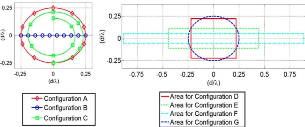
Figure 1. Different configurations and their areas.
obtain the same analogy, being equal to the distance of the furthest dipole to the center. The spiral is defined to have two turns on the center .[4]
The new four Configurations (D, E, F, and G) have a restricted area for placing the radiating elements, with a surface equal to the one occupied by Configuration A (circle with surface
S= r2xn. In the fourth one (Configuration D), the radiating elements are placed within a square, with side/ = r x yGr in order to have the same surface. In the fifth one (Configuration E), the radiating elements are placed within a rectangle, with /1 = 2 x r x \fn and with
/2 = 0.5 x r x \fn. Then, the surface is the same as in other configurations. In the sixth one
(Configuration F), the radiating elements are placed within another rectangle, with ^ = 4 x r x \[x and with /2 = 0.25 x r x \[x. Again, the surface is the same as in the other
configurations. Finally, in the seventh one (Configuration G), the elements have been placed in an optimum way within a circle, with the same radius as in Configuration A. The different configurations are shown in Figure 1.
3. Optimization
The Genetic Algorithm is a stochastic optimization algorithm which is at the same time robust and versatile. This GA has been used previously in [11 ] to obtain the optimum corre-lation functions. The spatial location of each element is a variable that needs to be optimized. The routine calculates the Capacity with the model of section. In this work, the optimization is limited to 1000 generations due to time constraints. The configuration of GA is different for simulation with 3-6 elements than for simulation with 7-10 elements. The ending con-dition is changed for 7-10 elements letting thefinalization of the optimization with softer conditions. For that reason, it is possible that this solution may be still improved.
3.1. Spatial optimization
- Conf. A Conf. B Conf. C Conf. D Conf. E Conf. F Conf. G
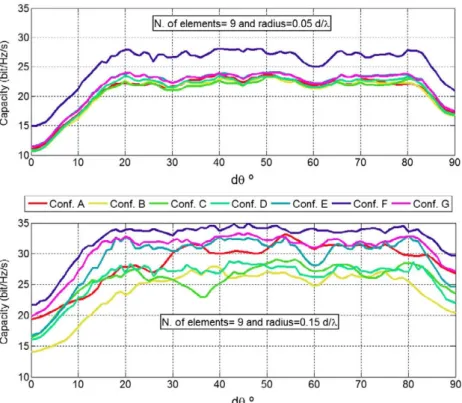
Figure 2. Capacity vs. d0for different configuration with number of elements equal to 9 and different radius (0.05 and 0.15 d/A).
from 2 to 10 with different radius, ranging from 0.07 d/A to 7 d/A [d is the distance between adjacent elements and A is the wavelength). The results were centered on a small range of radiuses (up to 0.3 d/A) because with more spatial distance the elements are decorrelated due to spatial diversity only and thus, the polarization optimization is not needed.
In Figure 2, the capacity vs. dd, for all configurations with radius = 0.05 d/A and the number ofelements = 9 (a), and with radius = 0.15 d/A and the number of elements = 9(b). Figure 2
illustrates that the performance of all the possible configurations with a small radius is quite similar except for Configuration F, which has more capacity, as the elements can be moved further away (in the diagonal of this rectangle). This occurs because in this small area it is difficult to distribute the elements efficiently. However, when the radius is increased, the optimization Configurations (D, E, F, and G) perform better than the configurations without it (A, B, and C). This difference is reduced when the radius is greater because it is easier to locate the elements in a bigger area. When the radius is equal to 0.15 d/A the capacity reached for all the options that combine spatial optimization with TPD technique is greater than the configurations with no spatial optimization. The curves are approximately flat except for very small angles (or very high), wherein the gain provided by the polarization diversity is very small.
O 10 20 30 40 50 60 70 80 90
dG°
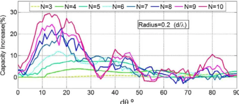
Figure 3. Capacity increase vs. d0 for different number of elements (3-10) and radius = 0.2 d/X.
in which the maximum capacity (flat zone) is reached between these devalues.To summarize, it can be stated that for a high number of elements and small areas (the most critical case), the available space to locate the elements is the most important factor in determining per-formance. However, with a small number of elements, performance for different configura-tions is very similar.
Figure 3 demonstrates the increment of capacity vs. dd, for Configuration G (circle with space optimization) regarding the Configuration A (circle with element at the perimeter), for radius = 0.2 d/X and different numbers of elements. In this graph, it can be seen that the greatest increase in capacity always occurs for a high number of elements (up to 30% in some cases). It is also clear that, for a large number of elements, sometimes the TPD technique works very well for Configuration A (for example when the angle = 45°) and it is very difficult to increase the capacity. Note that the largest increase in capacity occurs for dd between 10° and 20°. This is because the spatial optimization is able to combine the small benefit of polarization diversity in the best way.
In addition, it is remarkable that as long as the radius is increased, the increasing capacity is obtained until this radius is equal to 0.2 d/X. For this radius and beyond, the capacity increase begins to reduce. This is because the capacity of Configuration G has reached the maximum capacity with the radius equal to 0.2 d/X and cannot continue growing; meanwhile the capacity of Configuration A continues increasing. Thus, the percentage of increase in capacity is reduced. Finally, it is important to note that some values of Capacity Increase are negative, this occurs for a high number of elements and in this situation optimization cannot research the optimum placement.
3.2. Statistical study of spatial optimization
- Conf A Conf. B Conf. C Conf. D Conf. E Conf. F Conf. G
1.5
V 1
0.5
0
(a) N=3 1-5|(b)N=5t; 1
0.5
1 II fi ."..„,'
0 20 40 60 80
de
0 20 40 60 80
de
H. 0.5
(d) N=9 , t = 2 =
IMlllhÍLíJ.
20 40 60 80
d9
0 20 40 60 80
d0
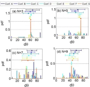
Figure 4. Pdf vs. dQand box-plot with (a) no. of elements = 3, (b) no. of elements = 5, (c) no. of elements = 7 and (d) no. of elements = 9.
Table 1. Mean of d9/Standard deviation of d9.
Number of elements
A B C D E F G 3 67/21 59/16 54/16 62/1 59/2 58/2 61/0 4 47/30 56/13 42/5 43/1 43/1 43/2 43/1 5 63/21 55/10 57/24 70/5 68/3 68/3 72/1 6 54/19 55/13 42/19 45/15 37/12 41/19 34/9 7 64/14 62/11 61/23 54/19 49/14 49/13 52/18 8 66/13 58/9 58/21 52/9 49/9 50/9 58/11 9 58/16 55/11 51/12 39/12 46/9 50/13 47/16 10 62/18 56/11 45/11 46/12 44/14 43/12 51/14
According to this low level of standard deviation, there exists one optimum d8 when spatial location is optimized. For more details, Table 1 provides the mean d6 and the standard deviation of d0.This table is very useful in order to extract some design rules in the following section.
5 6 7 Number of elements
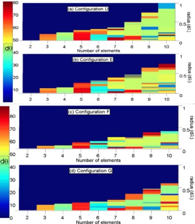
Figure 5. A 3D-contour plot of the d0 vs. radius (dA) vs. number of elements for Configuration D (a), Configuration E (b), Configuration F (c) and Configuration G (d).
radius (dlX)
Figure 6. A 3D plot of the capacity increase (%) vs. radius (dA) vs. number of elements for Configuration D (a), and Configuration E (b).
3.3. Double optimization (spatial-angular)
with double optimization related to the bestTPD configuration (with spatial optimization included). It is important to note that big capacity increases are not obtained with this new optimization (a maximum 3.6% in some cases). It is also noticeable that the increase is pro-duced when the radius is small and the number of elements is high. It is important to notice that the optimum polarization strategy always has more available capacity than the best TPD configuration because all TPD options can be found with GA. These results bring us to the following section where the best design option is discussed and some design rules are formulated.
4. Discussion
This section discusses the results obtained through space optimization, emphasizing the
d6s for which the maximum capacity was obtained. Considering this, some design rules can
be extracted and defined. In addition, the best option to reach the maximum capacity in small areas is discussed. As is observed, the extra polarization optimization does not increase the capacity obtained with the bestTPD option by more than the 3.6%.Therefore, the com-putational cost of the double optimization is not fully justified. Moreover, as shown in Figure
5, for a particular number of elements, the same polarization configuration is always chosen by the optimization algorithm in order to reach the maximum capacity. Considering this and the small increase in capacity with the double optimization, it is possible to suggest some design rules. These designs rules will be useful for designers in that they can implement the best TPD option and obtain a capacity very near to the maximum. The designs rules extracted for the polarization of the antennas are:
• For MIMO systems with three antennas, a d6 value around 60° should be used (the predominant color is orange).
• For MIMO systems with four antennas, a d6 value around 45° should be used (the pre-dominant color is green).
• For MIMO systems with five antennas, a d6 value around 70° should be used (the pre-dominant color is red).
• For MIMO systems with six antennas, a d6 value around 30° should be used (the pre-dominant color is blue).
• For MIMO systems with 7, 8, 9, or 10 antennas and the intermediate radius value, 45° should be used (the predominant color is green).
However, in other conditions, each spatial configuration works better with a different d6 and it is not possible to extract any particular design rule (for example, with 9 or 10 elements anda large radius, the color range is wider).This data is also reflected in Table 1 where a low standard deviation is obtained for 3,4, and 5 elements.
5. Conclusions a n d future w o r k
with small radiuses and a large number of elements, which is the usual situation for 4G technologies such as LTE. In addition, this article demonstrates that the effectiveness of the spatial optimization depends on the TPD configuration and the area to be occupied by the elements. Thus, spatial optimization increases the MIMO capacity. Furthermore, a double spatial-polarization optimization was undertaken. However, when a good strategy for diver-sity is chosen (TPD near 45° and elements located in the perimeter) the improvement through optimization is minimal. According to this, the optimal design of radiating elements in MIMO systems is either to locate the elements on the perimeter or to use a TPD technique with d6 between 45° and 60°, or both. Moreover, some more specific design rules are identified where the devalues work better in particular cases. For insta nee, for 4 elements the optimum
d8 is 60° and this d8 value also works optimally with 9 elements and in a medium-sized area.
Disclosure statement
No potential conflict of interest was reported by the authors.
References
[1 ] Rowell C, Lam EY. Mobile-phone antenna design. IEEE Antennas Propag. Mag. 2012;54:14-34. [2] Valenzuela-ValdésJF, Garda-Fernández MA, Martínez-González AM, etal. The role of polarization
diversity for MIMO systems under Rayleigh-fading environments. IEEE Antenna Wireless Propag. Lett. 2006;5:534-536.
[3] Valenzuela-Valdés JF, Garda-Fernández MA, Martínez-González AM, et al. Evaluation of true polarization diversity for MIMO systems. IEEE Trans. Antennas Propag. 2009;57(9):2746-2755. [4] Valenzuela-Valdés JF, Manzano MF, Landesa L. Deepening true polarization diversity for MIMO
system. IEEE Antennas Wirel. Propag. Lett. 2012;11:933-936.
[5] Zhang Z, Ye Z, Jiang W. Optimal antenna placement in distributed antenna systems. J. Syst. Eng. Electron. 2012;23:467-472.
[6] Park E, Lee S, Lee I. Antenna placement optimization for distributed antenna systems. lEEETrans. Wirel. Commun. 2012;11:2468-2477.
[7] Forooshani AE, Lotfi-Neyestanak AA, Michelson DG. Optimization of antenna placement in distributed MIMO systems for underground mines. lEEETrans. Wirel. Commun. 2014;1 3:4685-4692
[8] Hafiz H, Aulakh H, Raahemifar K. Antenna placement optimization for cellular networks. 26th Annual IEEE Canadian Conference on Electrical and Computer Engineering (CCECE), 2013; 2013 May 5-8; Regina, Canada, p. 1-6
[9] Liang H, Wang B, Liu W, etal. A novel transmitter placement scheme based on hierarchical simplex search for indoor wireless coverage optimization. lEEETrans. Antennas Propag. 2012;60:3921-3932.
[10] Valenzuela-Valdés JF, Martínez-González AM, Sánchez-Hernández D. Estimating combined correlation functions for dipoles in Rayleigh-fading scenarios. Antennas Wirel. Propag. Lett. 2007;6:349-352.