Bias Estimation for Evaluation of ATC surveillance
systems
1
Juan A. Besada, Gonzalo de Miguel, Paula Tarrío,
Ana Bernardos
GPDS-CEDITEC
Universidad Politécnica de Madrid
Madrid, España.
besada@grpss.ssr.upm.es
Jesús García
GIAA
Universidad Carlos III de Madrid
Madrid, España
jgherrer@inf.uc3m.es
1This work was funded by contract EUROCONTROL’s TRES, CICYT TSI2005-07344, CICYT TEC2005-07186
Abstract - This paper describes an off-line bias estimation and correction system for Air Traffic Control related sensors, used in a newly developed Eurocontrol tool for the assessment of ATC surveillance systems. Current bias estimation algorithms are mainly focused in radar sensors, but the installation of new sensors (especially Automatic Dependent Surveillance-Broadcast and Wide Area Multilateration) demands the extension of those procedures. In this paper bias estimation architecture is designed, based on error models for all those sensors. The error models described rely on the physics of the measurement process. The results of these bias estimation methods will be exemplified with simulated data.
Keywords: Bias estimation, Air Traffic Control, ADS-B, Multilateration.
1
Introduction
TRES (Trajectory Reconstruction and Evaluation Suite) will become in the near future a replacement for some parts of current versions of SASS-C (Surveillance Analysis Support System for Centres) suite [1]. This is a system used for the performance assessment of ATC multisensor/multitarget trackers. This paper describes the overall architecture of the assessment system, and details some of its elements related to opportunity trajectory reconstruction.
Opportunity trajectory reconstruction (OTR) is a batch process within TRES where all the available real data from all available sensors is used in order to obtain smoothed trajectories for all aircraft in the area of interest. It requires accurate measurement-to-reconstructed trajectory association, bias estimation and correction to align different sensor measurements, and adaptive multisensor smoothing to obtain the final interpolated trajectory. It should be pointed out that it is an off-line batch process potentially quite different to usual real time
data fusion systems used for ATC. Data processing order and processing techniques will be different.
In fact, one of the main uses of TRES is the evaluation of the performance of real time multisensor-multitarget trackers used for ATC, when they are provided with the same measurements as TRES. OTR works as a special multisensor fusion system, aiming to estimate target kinematic state, in which we take advantage of knowledge of future target position reports (smoothing).
TRES must be able to process the following kinds of data: • Radar data, from primary (PSR), secondary (SSR),
and Mode S radars, including enhanced surveillance. • Multilateration data from Wide Area Multilateration
(WAM) sensors.
• Automatic dependent surveillance (ADS-B) data. The complementarity nature of these sensor techniques allows a number of benefits (high degree of accuracy, extended coverage, systematic errors estimation and correction, etc.) and brings new challenges for the fusion process in order to guarantee an improvement with respect to any of the sensor techniques used alone. An important novelty is the integration of traditional ground based surveillance (PSR/SSR radars) with modern sensors such as WAM, with increased accuracy, and airborne sensors providing extended detection capability (velocity and maneuvers). The fusion of all measurements requires new solutions and a robust process that considers detailed characteristics of all data sources and checks their consistency before being fused.
The two basic aspects for estimating the reference trajectory are the development of appropriate models for sensor errors and target behavior. The model of sensor errors should address the probability density function (systematic and random components), to be exploited in the reconstruction process. Regarding the model of target behavior, it has been described in some previous works, and it is based in a practical implementation of the optimal smoother [1] and taking advantage of physical motion models tuned for aircraft flying in controlled airspace.
Much effort has been devoted in the last years to the definition of bias estimation procedures for multisensor multitarget tracking systems (among others [2][3][4][5]). These efforts have been mainly concentrated, in Air Traffic Control environments, to radar bias estimation and correction, as they are the most widely used sensors for this applications.
With the advent of new families of sensors the means for bias estimation must be extended. In this paper we propose and evaluate methods for this estimation, for en-route or terminal area (TMA). Those methods are based on the definition of error models for the sensors, and propose an architectural framework for bias estimation potentially extensible to other applications.
The paper starts with the definition of those error models, and then describes and justifies the bias estimation architecture, providing mathematical derivations of the different stages.
Finally, some results from simulated scenarios are provided, showing the convergence of the different bias estimation stages, and the effect over the tracking system.
2
Sensor Error models
Next we will define the error models for bias estimation for the different sensors previously described.
It should be noted that some of these bias terms are surely changing in time, at a rate dependent on propagation changes, other sensor calibration means (as station synchronization procedures for multilateration). A real time system trying to cope with these terms should define means to either:
• Forget sensor bias over time.
• Include models with changing bias in the estimation procedures.
In this paper we will assume constant biases.
2.1
ATC Radar Error models
There are mainly two types of radars used in ATC, primary (PSR) and secondary (SSR and Mode S) radars. They measurement range and azimuth, and in the case of SSR or Mode S, they also receive height from the aircraft barometer.
In the Mode-S and conventional secondary radar error model, k-th range-azimuth measurement (Rk, θk) include
the terms in (1):
) ( ) ( cos ) ( sin ) ( ) ( ) ( ) 1 ( 2
1 k k n k
k k n R R k R K R id id id k R j id k θ θ θ θ θ θ θ θ = +Δ +Δ +Δ + + Δ + Δ + + = (1) where:
(Rid(k), θid(k))are the ideal target position for the k-th
measurement, expressed in local polar coordinates. • ∆R: radar range bias.
• K is the gain of range bias.
• ∆Rj: transponder induced bias of j-th aircraft,
different for each aircraft.
• ∆θ is the azimuth bias.
• (∆θ1,∆θ2) are the values which characterize the
radar’s azimuth eccentricity, related with maximum eccentricity and angle of maximum eccentricity. • (nR(k),nθ(k)) are measurement noise errors.
Primary radar has the same model except the lack of ∆Rj
term. We assume transponder antennae are pretty near the center of the aircraft.
When we translate this measurement to stereographic plane, we would use a quite exact non-linear coordinate transformation method [6]. This method implements a function we will call fRadar(.). So, to project error terms
into stereographic plane, we can make first order approximation of this transformations, and we will have:
⎥ ⎦ ⎤ ⎢ ⎣ ⎡ + ⎥ ⎥ ⎥ ⎥ ⎥ ⎥ ⎥ ⎥ ⎦ ⎤ ⎢ ⎢ ⎢ ⎢ ⎢ ⎢ ⎢ ⎢ ⎣ ⎡ Δ Δ Δ Δ Δ + ⎥ ⎦ ⎤ ⎢ ⎣ ⎡ ≅ ⎟ ⎟ ⎠ ⎞ ⎜ ⎜ ⎝ ⎛ ⎥ ⎦ ⎤ ⎢ ⎣ ⎡ = ⎥ ⎦ ⎤ ⎢ ⎣ ⎡ ) ( ) ( ) ( ) ( 2 1 0 , 0 , k n k n G K R R H k y k x R f y x R R j R id id k k Radar k k θ θ θ θ θ (2) where:
• xid(k), yid(k) is the ideal target position for the k-th
measurement.
• HR is the Jacobian of f (.) with respect to the
vector It is a 2x6
matrix, whose two first rows are equal, raising a potential observability problem in our bias estimation procedures.
Radar
[
ΔR ΔRj K Δθ Δθ1 Δθ2]
T.• GR is the Jacobian of fRadar(.) with respect to the
vector
[
nR(k) nθ(k)]
T. It is a 2x2 matrix.There is also a potential time bias, leading to an equivalent position bias aligned with velocity. Then, (X,Y) projected measurements will suffer an additional bias of the form:
(3) t V y y t V x x Y k k X k k Δ − = Δ − = 0 , 0 , where:
• (VX, VY) is the velocity vector of the target in this time.
• ∆t: is the time bias for the radar.
Finally, it should be noted there are collocated PSR-SSR and PSR-Mode S radars, for which we will define two virtual sensors, one for PSR and another one for the secondary radar.
2.2
ADS-B Error models
The k-th position measurement (xk, yk), obtained using the stereographic projection over latitude, longitude and height measurements, may be modelled as:
(3)
) ( )
(
) ( )
(
k n t V k y y
k n t V k x x
y j Y id k
x j X id
k
+ Δ − =
+ Δ − =
where:
• xid(k), yid(k) is the ideal target position for the k-th measurement.
• (VX, VY) is the velocity vector of the target in this time.
• ∆tj: is the time bias for j-th aircraft.
• nx(k), ny(k) are measurement noise errors
2.3
Wide area multilateration Error models
Wide area multilateration measurement performs Time Difference Of Arrival (TDOA) estimation to calculate target position. No matter the method used for position estimation, the basic measurements used to obtain the aircraft position are the times of arrival of the same signal emitted from this target. The bias of multilateration is a function of several variables, including:
• The geometry of the receiver(s) and transmitter(s) • The timing accuracy of the receiver system
• The accuracy of the synchronization of the transmitting sites or receiving sites. This can be degraded by unknown propagation effects.
It should be noted that the multilateration system has internal calibration means, as without them no position estimation would be possible. So we are dealing with remaining errors after this calibration. This is a subject still under active research, a description of the main error terms may be found in [7]. In this system we assume the bias changes in space are not too fast, and therefore we perform a discretization of the space in cells. Then, the k-th position measurement (xk, yk), obtained using the
stereographic projection over latitude, longitude and height measurements, may be modelled as:
(4)
) ( ) ( )
(
) ( ) ( )
(
k n n Y t V k y y
k n n X t V k x x
y Y
id k
x X
id k
+ Δ + Δ − =
+ Δ + Δ − =
where:
• xid(k), yid(k) is the ideal target position for the k-th measurement.
• (VX, VY) is the velocity vector of the target in this time.
• (∆X(n),∆Y(n)): is the X,Y bias for n-th cell in the cell list, equal for all aircraft.
• ∆t: is the time bias for all aircraft and cells.
• (nx(k), ny(k)) are the noise components in stereographic plane.
3
Bias estimation architecture
From the previous description it is evident there are three different kinds of bias terms:
• Terms dependent on sensor
• Terms dependent on the sensor-target pair • Terms only dependent on the target
The bias estimation procedure takes into account this fact, and is based on three steps:
• Track bias estimation: From all the available data from a given aircraft, integrated in a multisensor track, it obtains an estimation of all the bias terms from all sensors providing measurements to this track. These same measurements will be used for calculating aircraft trajectory, but this functionality will not be analyzed here. Only measurements obtained during constant velocity movement segments should be used. In next sections we will both describe the general method for this function, and provide the parameters needed to implement them given the previous error models. It should be noted that, in this stage, any observability problem will be addressed by estimating jointly the problematic variables. In later stages we will try to solve those problems. As important as obtaining a vector of bias estimates is obtaining a consistent measurement of its covariance matrix.
• Sensor bias estimation: This method integrates all track bias estimators in an efficient manner, to obtain sensor related biases. It assumes the previously described bias vectors are independent measurements (as they come from different aircraft measurements) of the sensor bias terms. Those measurements have a covariance matrix which, in most situations, is equal to the one obtained as result of track bias estimation. But, due to observability problems, and to the presence of target related biases, sometimes it is necessary to make some changes in these covariances. We will describe in later sections those modifications and the complete sensor bias derivation procedure.
• Target bias estimation: This is obtained for each aircraft, provided sensor related bias was previously corrected. This estimation must be performed either in parallel or almost in parallel with target tracking. In this paper we are not addressing the potential problems related to sensor integrity potentially leading to bias model mismatch. If those problems could arise, the procedure for bias estimation should be capable of detecting them and changing its behavior, not using this degraded sensor information for bias estimation (neither for tracking).
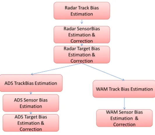
Due to current state of maturity of the deployed ATC measurement system, radar systems are in general assumed to be safer, while WAM and ADS-B systems have yet to show their operational validity. Due to that lack of expertise in the use of those new sensors, a conservative approach was taken, where the processing order is the one described next.
estimation and corrections are a prerequisite for those other sensors estimation.
Therefore, the order in which the all sensor and target biases are estimated and corrected is depicted in next figure.
Radar Track Bias Estimation
Radar SensorBias Estimation &
Correction Radar Target Bias
Estimation & Correction
ADS TrackBias Estimation
ADS Sensor Bias Estimation
ADS Target Bias Estimation &
Correction
WAM Track Bias Estimation
WAM Sensor Bias Estimation &
Correction
Figure 1: Bias estimation and correction algorithms Please note there are several similar processes (track bias estimations for each kind of sensor, sensor oriented bias estimation, target oriented estimation and correction). They all are based on a set of generic algorithms to be described next. ADS-B and WAM bias estimation have as a prerequisite the estimation of radar biases. This is a limitation of current OTR to be addressed in next versions.
3.1
Generic Track bias estimation
This block is in charge of calculating biases for all sensors feeding a given multisensor track. It is based on a Kalman filter with stacked parameters for:
• Target position. • Target velocity.
• Bias parameters to be estimated for all sensors feeding the multisensor track.
Each target is seen for a different set of sensors, and therefore the state vector of this Kalman filter is different. Even more, for a same given target, the set of sensors feeding its track changes in time, and therefore the meaning of the state vector is changing as it traverses the coverage of different sensors.
To reduce computational load, we converted the Kalman filter in a set of coupled filters by rearranging the information in the filter. The results are identical to those obtained in a Kalman filter for the estimation of all bias terms. Each of the bias estimates may be seen as a set of rows in the complete Kalman filter state vector. Using this, and the fact that each measurement comes only form one sensor, and therefore only these sensor bias terms are
projected into it, the Kalman filter may be arranged in a highly efficient manner. We arrange the complete bias estimate as a list of vectors (to be called estimate), the first containing the position (X,Y) and velocity (Vx,Vy) in
stereographic coordinates, and the others containing the bias estimate of each of the sensors. With this structure in mind, each time we add a measurement from a new sensor, with its own bias terms, we will add a new element in the estimate list.
X Y Vx
Vy
b11
b12
b13
b14
b21
b22
b23
b24
b25
b26
b21
b22
b23
b24
b25
b26
b11
b12
b13
b14
X Y Vx
Vy
estimate[0]
estimate[1]
estimate[2] Complete estimate vector
Figure 2: List of estimates in a track bias estimator Each element of estimate list could have a different size, as it will contain the bias terms potentially belonging to different kinds of sensors.
For the posterior calculation of sensor and target oriented bias terms we would need to be able to calculate not only the whole vector estimate from each target, but also its associated covariance matrix. We can arrange the covariance elements in a list of lists of covariances between the estimators in estimate list. As the complete covariance is a symmetric matrix, it is not necessary to save all the covariances, but only a part of them (roughly, one half). We would need to have access to all cross covariances between estimates. Imagine we call Ci,j the
cross covariance between estimate[i] and estimate[j]. It is clear, in this case, . We call this list of lists
covariance.
T j i i j
C
C
,=
,The list of lists indicated covariance has the structure in Figure 3. Two indexes are used to access each of the elements. It may be noted that Ci,j is, in this structure, in
C0,0 C0,1 C0,2
C1,1 C1,2
C2,2
covariance[0]
covariance[1]
covariance[2]
covariance[0] [1]
covariance[1] [1]
Figure 3: Structure of covariance list in local bias estimator
With these structures in mind, the track bias estimation performs the following procedure based on constant velocity movement segments (note we need some delay between real time and time to process measurements, in order not to process measurements in maneuvering conditions).
We then initialize the estimate and covariance lists. The position estimates (X and Y in Figure 2) in estimate[0] are set to the horizontal positions of the first measurement in the constant velocity segment. Then, the velocity estimates (VX and VY in Figure 2) are used to initialise a
rough estimate (based on monosensor measurements) of trajectory velocity. Then covariance[0][0] is initialised to C0,0, described in (5).
⎥ ⎥ ⎥ ⎥ ⎥
⎦ ⎤
⎢ ⎢ ⎢ ⎢ ⎢
⎣ ⎡
=
2 2 2 2
0 , 0
0 0 0
0 0
0
0 0 0
0 0 0
vel vel pos pos
C
σ σ σ σ
(5)
where
σ
pos andσ
velare constants for the adaptation of the algorithm.We must process in turn all constant velocity segments in a given trajectory. If we finished processing a segment, we must reinitialize the estimate[0] vector and all the
covariance[0][i] matrices. In the case of estimate[0] and
covariance[0][0] it must be done as with the first measurement of the first constant velocity segment. For the rest of the covariance[0][i] matrices (cross covariances between position/velocity vector and previously estimated sensor biases), we must initialize them to zero matrices.
For each measurement in the constant velocity segment we must check if it belongs to a sensor not previously processed for bias estimation or not. If it was not previously processed we must:
• Add a new element, with zero values, to estimate
list, which will contain the bias terms related to this sensor.
• Add new elements to all covariance lists, with zero values, at the final position.
• Add a new list, with only one matrix as element, to
covariance list of lists. The contents of this matrix are sensor type specific (let us call them Csensor).
They are diagonal matrices with quite big values in order to avoid having any impact of initialization over bias estimation.
Both in the cases the measurement processed comes from a new sensor and not, we must process it with the rearranged Kalman filter we are proposing. The filtering steps are as follows:
• Obtain the time since previous measurement filtering, to be called T.
• Calculate position prediction matrix F, as:
⎥ ⎥ ⎥ ⎥
⎦ ⎤
⎢ ⎢ ⎢ ⎢
⎣ ⎡
=
1 0 0 0
0 1 0 0
0 1 0
0 0 1
T T
F (6)
• Predict estimates: all estimate elements remain constant (we assume constant biases), but the one related with position:
estimate[0]=F*estimate[0] (7) • Predict covariances. Those covariance elements
related with position are the only ones which need to be changed. Those are the covariances in the first list of covariance:
o First the estimate[0] covariance need to be changed:
T F * [0][0] *
F
[0][0] covariance
covariance = (8)
o For the rest of terms the prediction takes the form:
covariance[0][j]=F*covariance[0][j] (9) • Calculate the bias projection matrix Hb, dependent of
the sensor model type, and of the measurement under analysis (details on it twill be provided in later sections). It must be pointed out that, in certain stages of the processing, when the bias terms have been corrected, we will use the data in the Kalman filter not including terms for this sensor and Hb will
be an undefined matrix (and all the terms related with it in further steps must be negelected)
• Define a matrix to be called Hpos of the form:
⎥ ⎦ ⎤ ⎢
⎣ ⎡
=
0 0 1 0
0 0 0 1
pos
H (10)
• Calculate the horizontal projection of the measured position (in stereographic plane). We will call this measurement xm.
• Calculate n as the index in estimate list of the sensor providing the measurement,
• Calculate the residual of the Kalman filter as:
[ ]
H[ ]
nH x
• Obtain the measurement covariance, projected in the horizontal plane, associated to the datum. This is a 2x2 matrix. It will be called R in next computations. • Calculate the residual matrix Sres as:
R + + + + = T b b T pos T b T b pos T pos pos res H * [n][0] * H H * [0][n] * H H * [0][n] * H H * [0][0] * H S covariance covariance covariance covariance (12)
• Calculate two lists of N matrices. We will call them B[i], with 0<=i<N, and BT[i]. To calculate them we will use two different methods, depending on the value of i:
o If i<n
T T b pos T T b pos H * i] -[i]n H * [0][i] BT[i] i] -[i][n * H [0][i] * H B[i] covariance covariance covariance covariance + = + = (13)
o If i>=n
T T b T pos T b pos H * n] -[i][i H * [0][i] BT[i] n] -[i][i * H [0][i] * H B[i] covariance covariance covariance covariance + = + = (14) • Calculate a list of Kalman gain matrices (K[i]) for the corresponding estimate element. It is calculated as: -1 res S * BT[i]
K[i]= (15)
• Calculate the filtered estimate. Using our lists, it may be done through a loop in which we perform independent updates of the estimate elements, and of all the terms in each row of the covariance
structure. The filtered estimate element must be updated. It is calculated as:
estimate[i]=estimate[i]+K[i]*res (16) • The filtered covariance structure must be updated.
To update each element in the row we must perform a new loop, with index 0<=j<N-i. The corresponding covariance elements must be updated as:
covariance[i][j]=covariance[i][j]-K[i]*B[i+j] (17) After processing all measurements from the multisensor track, we will obtain the estimate and covariance estimates.
Next we will detail the use of this filter within the OTR.
3.2
Radar track bias estimation
SSR, PSR and Mode S radars have their track bias estimated at a first stage, to perform global radar bias estimation. Those estimators will make only use of radar measurements, ADS or WAM measurements will not be used yet.
It should be noted that all local bias estimators are not estimating, when referring to the same SSR or Mode S virtual radars, the same values. The range bias term is different for each target, as it includes also the transponder delay, and this must be taken into account when the global estimates are derived. There is lack of observability of range bias and transponder delays terms separately, so the track bias estimator estimates the sum of both terms.
Then, for each virtual sensor the track bias estimate will have states for:
• Sum of Range Bias and Transponder delay for SSR and Mode S radars, or Range bias for PSR.
• Range Gain • Azimuth Bias
• Azimuth Eccentricity parameters. • Time stamp bias.
Provided HR is the matrix defined in (2), and we use (i,j)
notation to express the element in this matrix, Hb bias
projection matrix is of the form:
⎥ ⎦ ⎤ ⎢ ⎣ ⎡ − − = Y R R R R R X R R R R R
b H H H H H V
V H H H H H H ) 6 , 2 ( ) 5 , 2 ( ) 4 , 2 ( ) 3 , 2 ( ) 1 , 2 ( ) 6 , 1 ( ) 5 , 1 ( ) 4 , 1 ( ) 3 , 1 ( ) 1 , 1 ( (18) It contains all HR elements, but not repeating the second
element, as we calculate the sum of those two elements. (VX, VY) is the velocity vector of the target in this time.
At the beginning, it should be estimated from monosensor measurements. Note this matrix contained ideal values of range, azimuth, and height but we would use them to calculate the measurements.
3.3
Radar Sensor Bias Estimation and
correction
Radar global bias estimation is the process in charge of exploiting local bias estimators from radar data to obtain the following data for each radar of type PSR, SSR or Mode S:
• Range Bias • Range Gain • Azimuth Bias
• Azimuth Eccentricity. • Time stamp bias.
To do that, it implements a Kalman filter in which each local bias estimator is treated as a measurement of the bias terms from a group of sensors (those feeding the associated multisensor track), and with all global bias terms from all sensors in stacked in the state vector. Each local bias estimator comprises a different set of bias estimators from different sensors. The matching between local bias estimator and global bias estimators, and between them all and sensor model bias, is therefore critical in this system.
the range bias for Mode S and secondary radar, and reinterpret the result as an estimate of the range bias with incremented uncertainty. This uncertainty is related with the lack of knowledge of transponder delay, and therefore all SSR and Mode S sensors range bias local bias estimate will have a correlated error term (different in SSR and Mode S modes).
After bias estimation, biases are corrected and all measurements retransformed to stereographic plane.
3.4
Radar target bias estimation and
correction
This process is in charge of estimating Mode S and conventional transponder time delay, expressed in meters. This is what we called a target bias estimator. To do so it performs an estimation similar to that of the local bias estimation for radars, based on PSR, SSR and Mode S radar data. To do so, it uses data with global biases from radar corrected, and uses bias model with two terms: • SSR transponder delay
• Mode S transponder delay
The filter also contains four additional states, the position (X,Y) and velocity (Vx,Vy) in stereographics estimates, and the others containing the bias estimate of each of the sensor. Position is initiated with the first measurement in each straight line, and reinitiated for each straight line, with a velocity given from straight line calculation method. All SSR sensors share the same SSR transponder delay, and all Mode S measurements from all sensors have the same Mode S transponder delay. PSR data has no transponder delay at all. This is taken into account in the Kalman filter modelling, which additionally assumes constant transponder delay.
After this estimation, all SSR and Mode S radar data are corrected with the offset corresponding to its target (if available). Once again, after bias estimation, biases are corrected and all measurements retransformed to stereographic plane.
3.5
ADS Track Bias Estimation
ADS local bias estimation is based on the use of ADS position measurements and radar (PSR, SSR and Mode S) measurements. Radar measurements used here have their sensor related and target related bias terms corrected. Therefore, it is like, at this step, they suffered no bias, and the ADS bias estimator will find the necessary offsets to get aligned with it.
Track bias estimation estimates, for each target, only: • Target Time bias
The related Hb bias projection matrix for ADS
measurements takes the form:
⎥ ⎦ ⎤ ⎢ ⎣ ⎡
− − =
Y X
b V
V
H (19)
where (VX, VY) is the velocity vector of the target in this
time. After some measurements are processed in the bias estimation Kalman filter it can be obtained from the third and fourth element of estimate[0].
Radar measurements are asumed to be bias free, and so no Hb value needs to be defined for them.
3.6
ADS Sensor Bias Estimation
Track ADS bias estimation may suffer from a problem. If a given aircraft has no straight line segment, the system will not be able to provide time stamping bias. So we will calculate an average time bias for all ADS, and mix it with the available information from all sensors taking into account its relative qualities.
3.7
ADS Target Bias Estimation and
Correction
For the data from a target with constant velocity segments it will calculate a good enough bias estimate, and so the corrections will be mainly based on the own local estimate.
For targets with no constant velocity segments it will be used to correct the average performed in the global bias procedure. The idea is providing a value logical for the user as output, although the effects on bias correction will be negligible.
Therefore, bias estimation estimates, for each target, bias terms are:
• Target Time bias
Those bias estimates are used to correct all ADS measurements, which are then retransformed to stereographic plane.
3.8
WAM Track Bias Estimation
WAM track bias estimation is based on the use of WAM position measurements and radar (PSR, SSR and Mode S) measurements. Radar measurements used here have their sensor related and target related bias terms corrected. Therefore, it is like, at this step, they suffered no bias, and the WAM bias estimator will find the necessary offsets to get aligned with it.
This local estimator is special, as each target will contain only the terms related with the WAM error cells it is traversing, and from which there are WAM measurements (according to its associated WAM measurements). For each cell, the terms are:
• Local to sensor X bias • Local to sensor Y bias • Time bias
Note all cells bias related terms will contain a time bias estimate, although time bias is actually unique for all cells.
The bias estimation terms for track bias estimation are the values of the biases at each cell. It should be noted that for a given track, it is possible not to receive a signal, in any of its measurements, from a given cell. There would be two possibilities:
• Increase the length of the bias vector as we receive measurements from new cells.
The method used in OTR is based on the first approach, as the number of cells may be huge. What we did was defining a virtual subsensor for each WAM cell, where
Figure 4: List of estimates in sensor bias estimation Radar
number and type
Range noise (m)
Estimated Range noise (m)
Range Bias (m)
Estimated Range Bias (m)
Estimated Range bias 95% band (m) 1-PSR 110 120.40 50 17.73 ±21.4
2-MS 74 73.79 0 -14.4 ±29
2-SSR 74 78.04 0 -16.71 ±33.4
3-SSR 74 73.60 25 15.87 ±26.7
4-SSR 74 71.27 25 -16.75 ±26.9
5-MS 74 76.92 150 163.26 ±27.1
5-SSR 74 72.93 150 195.01 ±38.1
⎥ ⎦ ⎤ ⎢
⎣ ⎡
− − =
X X
b V
V H
1 0
0
1 (20)
Each time the target enters a new cell, it is as if we were using a new sensor.
3.9
WAM Sensor Bias Estimation and
Correction
Global WAM bias estimation obtains the result from local bias estimators and obtains a unique time bias for the whole sensor by mixing all time biases, and X-Y offsets per cell. It is implemented with a Kalman filter in which each local bias estimator from WAM is assumed to be a measurement of the error cell X-Y terms and of the time offset.
Table 1: Simulated noise and bias estimation results In last table we summarize noise and bias estimation results, for selected radars and coordinates. Having a same number and different types means those are different virtual sensors from a same real physical sensor.
Quite often the 95% band of error in bias estimation is not respected due to:
Therefore, the each cell, the resulting global bias terms
are: • Approximations in the bias processing
• Local to sensor X bias • Presence of transponder bias, whose average is mixed with the radar bias
• Local to sensor Y bias
But it is clear from those and other results the bias estimation is converging to values near the actual ones. In addition, there is a common bias estimate being shared
by all cells within the sensor: • Time bias
5
References
All those bias terms values are corrected for all WAM measurements, given a sensor and the cell it belongs to. Of course, it also demands a reprojection of the measurements.
[1] Juan A. Besada, Gonzalo de Miguel, Andrés Soto, J. Garcia, R, Alcazar, E. Voet. “TRES: Multiradar-Multisensor Data Processing assessment using Opportunity Traffic”. 2008 IEEE Radar Conference. Rome.
4
Results and conclusion
Next we are describing some noise and bias estimation results from a simulated data example, with error models consistent with the described models. Of course, those results are dependent on actual position of simulated radars and relative geometry of targets. This is a scenario with 61 aircraft with a mixed fleet with SSR and Mode S transponders, and Mode S, SSR and PSR radars.
[2] A. Rafati et al., “Asynchronous Sensor Bias Estimation in Multisensor-Multitarget Systems,” Multisensor Fusion and Integration for Intelligent Systems, 2006 IEEE International Conference on, 2006, págs. 402-407.
[3] X. Lin, Y. Bar-Shalom, y T. Kirubarajan, “Multisensor multitarget bias estimation for general asynchronous sensors,” Aerospace and Electronic Systems, IEEE Transactions on, vol. 41, 2005, págs. 899-921.
In next figure, the radar coverage is depicted in colors, while white lines depict simulated aircraft trajectories.
400 600 800 1000 1200 1400 1600 1800 400
600 800 1000 1200 1400
Km (east)
K
m
(
nor
th)
pr1 ms1 sr2 sr1 ms2
sr3 sr4 pr2 AD-1
AD-2
WM-1
pre005 pre006
pre007
pre008 pre009
pre010
pre011
pre012 pre021
pre022 pre154 pre155
pre156 pre157 ses24
ses25
ses26
ses27 ses28
ses29 ses30
ses31
ses32 ses33 ses34 ses35
ses36 ses37
ses38 ses39
ses40
ses41
ses42 ses43
[4] J. Besada Portas, J. Garcia Herrero, y G. de Miguel Vela, “Radar bias correction based on GPS measurements for ATC applications,” Radar, Sonar and Navigation, IEE Proceedings -, vol. 149, 2002, págs. 137-144.
[5] Pyung Soo Kim, “Separate-bias estimation scheme with diversely behaved biases,” Aerospace and Electronic Systems, IEEE Transactions on, vol. 38, 2002, págs. 333-339.
[6] L. Paradowski y Z. Kowalski, “An effective coordinates conversion algorithm for radar-controlled anti-aircraft systems,” Microwaves and Radar, 1998. MIKON '98., 12th International Conference on, 1998, págs. 771-775 vol.3.