Extensions of fundamental hub location models

Texto completo

(1)PONTIFICIA UNIVERSIDAD CATÓLICA DE CHILE ESCUELA DE INGENIERÍA. EXTENSIONS OF FUNDAMENTAL HUB LOCATION MODELS. ARMIN MAURICIO LÜER VILLAGRA. Thesis submitted to the Office of Research and Graduate Studies in partial fulfillment of the requirements for the Degree of Doctor in Engineering Sciences Advisor: VLADIMIR MARIANOV KLUGE. Santiago de Chile, October, 2015 © 2015, Armin Mauricio Lüer Villagra.

(2) PONTIFICIA UNIVERSIDAD CATÓLICA DE CHILE ESCUELA DE INGENIERÍA. EXTENSIONS OF FUNDAMENTAL HUB LOCATION MODELS. ARMIN MAURICIO LÜER VILLAGRA. Members of the Committee: VLADIMIR MARIANOV KLUGE JORGE VERA ANDREO JAIME BUSTOS GÓMEZ GABRIEL GUTIÉRREZ JARPA ELENA FERNÁNDEZ ARÉIZAGA JORGE VÁSQUEZ PINILLOS Thesis submitted to the Office of Research and Graduate Studies in partial fulfillment of the requirements for the Degree of Doctor in Engineering JORGE VÁSQUEZ PINILLOS Sciences. Santiago de Chile, October, 2015. © 2015, Armin Mauricio Lüer Villagra.

(3) To my parents Armin and Nelly.. ii.

(4) ACKNOWLEDGEMENTS. To Dr. Vladimir Marianov for letting me to work with him. His support, guide and wisdom has helped me a lot to complete this thesis and doctorate program. He has showed me not only how to do research and progress in science and academia, but also to be loyal, patient, fair and kind with everyone. I hope to continue working with him in the future, besides his expertise and wise advice, because I appreciate him a lot and enjoy working along with him. To my parents, Armin and Nelly, for their unconditional love and support, and for always encourage me, from my first years up to now. To Lorena, for being as she is, so kind and intrinsically lovely, and for making me a happier, more relaxed and better person. To my mentor, colleague and friend, Dr. Jaime Bustos, for introducing me to Operations Research, and for its guide and kind friendship. For the enjoyable years at LIA-DIS, and his support along the process of my undergraduate and doctorate studies. To my colleagues of the doctorate program with whom I have spent lots of hours discussing our topics, making progress, talking, relaxing, or just making the time more enjoyable. Special thanks to Germán, Ana, Guillermo, Andrés and César for their friendship. To my friends Rodrigo D., Bárbara, Jovanka, Felipe F., Evelyn and Marcela for the good times, and for their support (and patience) during all these years. Special thanks to Los Perpetradores: Nicolás, Andrés and Francisco, for their friendship since elementary school.. iii.

(5) To Mg. Pedro Valenzuela, Dra. Sonia Salvo and Dr. Mario Gúzman at Universidad de La Frontera for their kind advice and teaching. To Carlos, Virginia and Karina for being so kind with all the students of the Department of Electrical Engineering. To Betty, Gianina, Karina, Ana María, Jessica and Mary for the help, patience and kindness all these years, and for simplifying our lives a lot at the Department of Electrical Engineering. The same to Karina, Jacqueline, Ximena and Pilar at the Department of Industrial and Systems Engineering. To Debbie, Gloria, Fernanda, Danisa and Nicole, for their administrative support, patience and advice at DIIPEI. To Institute Complex Engineering Systems, that supported this research through Grants ICM- MINECON P-05-004-F and CONICYT FBO16. To CONICYT for awarding me with scholarship 21100276 of 2010 to follow a doctorate program in Chile, and FONDECYT to partially support this research through Grant 1100296. In summary, I thank everyone who have given me their support in any way during this journey.. iv.

(6) CONTENTS. 1.. 2.. Introduction ............................................................................................................ 1 1.1.. Competitive models .................................................................................... 2. 1.2.. Efficient solution approaches to the fundamental models .......................... 3. 1.3.. Cost structures for hub-and-spoke networks .............................................. 4. 1.4.. Use of different inter-hub network topologies ........................................... 7. 1.5.. Thesis contributions .................................................................................... 9. A competitive hub location and pricing problem ................................................. 11 2.1.. Introduction .............................................................................................. 12. 2.2.. A Competitive Hub Location and Pricing Problem.................................. 17. 2.3.. Solution approach ..................................................................................... 20 2.3.1. Genetic algorithm......................................................................... 22 2.3.2. Pricing problem ............................................................................ 24. 2.4.. Computational experiments and discussion ............................................. 27 2.4.1. The role of inter-hub economies of scale on the entrant’s profit . 28 2.4.2. Optimal pricing decisions ............................................................ 32 2.4.3. Entrant’s network structure .......................................................... 36. 2.5. 3.. Conclusions .............................................................................................. 40. A modelling framework for strategic airline network design .............................. 43 3.1.. Introduction .............................................................................................. 44. 3.2.. Literature review....................................................................................... 45 3.2.1. Economies of scale in the airline industry ................................... 45 3.2.2. Hub location and network design models .................................... 49. 3.3.. Modelling framework for strategic airline network design ...................... 57 3.3.1. Framework structure .................................................................... 59 v.

(7) 3.3.2. MIP model for the airline network design problem ..................... 60 3.4.. Computational experiments ...................................................................... 66 3.4.1. Economies of scale ...................................................................... 67 3.4.2. Upper bound on the total distance travelled ................................ 69 3.4.3. Fleet composition ......................................................................... 71 3.4.4. Operational constraints ................................................................ 73 3.4.5. Flying material specifications ...................................................... 75. 3.5. 4.. Concluding remarks .................................................................................. 77. On single-allocation p-hub median location problems with flow threshold-based discounts and economies of scale ......................................................................... 79 4.1.. Introduction .............................................................................................. 80. 4.2.. The problem .............................................................................................. 85 4.2.1. Exact model ................................................................................. 86 4.2.2. Heuristic procedure ...................................................................... 88. 4.3.. Computational Experiments and Discussion ............................................ 90 4.3.1. Existence of economies of scale .................................................. 91 4.3.2. Sensitivity in the flow threshold T ............................................... 92 4.3.3. Effect of the discount factor ......................................................... 93 4.3.4. Comparison of our exact model with the fundamental p-hub model 96 4.3.5. Heuristic performance .................................................................. 97 4.3.6. Summary .................................................................................... 100. 4.4.. Concluding remarks ................................................................................ 100. 5.. Conclusion .......................................................................................................... 101. 6.. Bibliography ....................................................................................................... 104. vi.

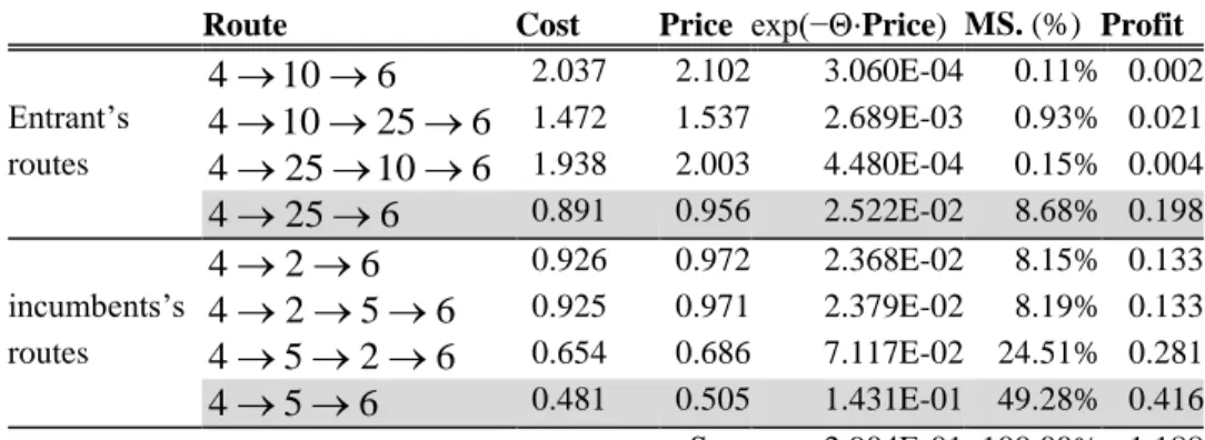
(8) LIST OF TABLES Table 2-1. Optimal pricing by the entrant, with cost advantage, Θ = 15.39, Δ = 0.05, α = 0.2, for the (8,3) OD pair. Entrant’s hubs on nodes 10 and 25, and incumbent’s hubs on nodes 2 and 5. ................................................ 34 Table 2-2. Optimal pricing by the entrant, without cost advantage, Θ=3.85, Δ=0.05, α=0.2, for the (4,6) OD pair. Entrant’s hubs on nodes 10 and 25, and incumbent’s hubs on nodes 2 and 5. ................................................ 36 Table 2-3. Number of open hubs (# hubs) and arcs (# arcs), running time (Time), Entrant’s Profit and Incumbent’s Income, for all scenarios and values of q. ............................................................................................................... 40 Table 3-1. KPIs obtained by limiting the maximum number of large planes ( P l ) available in the base instance. ....................................................................... 72 Table 3-2. KPIs obtained by limiting the maximum number of available small planes ( P s ) in the base instance. ................................................................... 72 Table 3-3. Results on base instance with Pl  4 and P s  18 , including constraints (19) or (20). ................................................................................. 73 Table 3-4. KPIs obtained by changing the autonomy of small airplanes ( Au s ) in the base instance. ........................................................................................... 76 Table 3-5. KPIs obtained by changing the autonomy of large airplanes ( Au l ) in the base instance. ........................................................................................... 77 Table 4-1. Comparison between our exact model and the fundamental model, for α=0.5. ............................................................................................................ 98 vii.

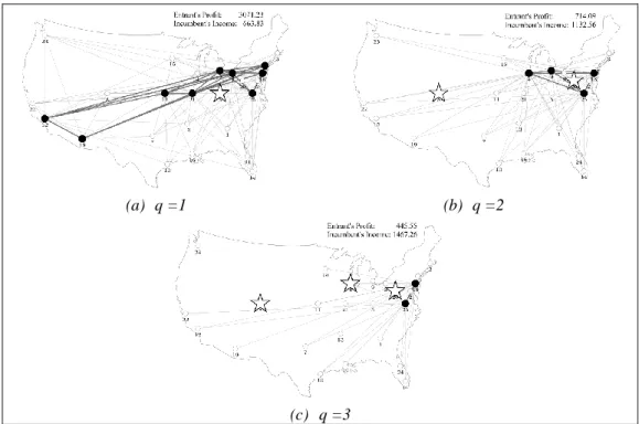
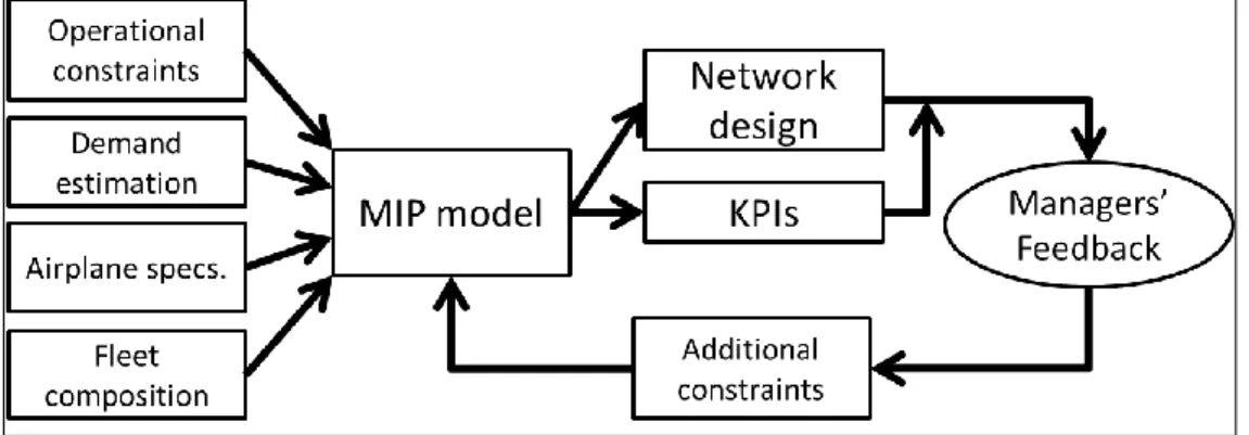
(9) LIST OF FIGURES Figure 2-1. (a) Two partial solutions with |N|=4, to be used with the proposed genetic algorithm. After applying 1-point: (b) row crossover, (c) column crossover. ........................................................................................ 23 Figure 2-2. Entrant’s objective function value as a function of α, with Δ=0.05 and Θ = 5.78. ...................................................................................................... 30 Figure 2-3. The effect of sensitivity to price differences on the entrant’s profit. ........... 31 Figure 2-4. Entrant’s objective function value as a function of σ, with Δ=0.05, for different values of α. .................................................................................... 32 Figure 2-5. Incumbent’s and entrant’s market share and profit, for different values of entrant’s margin over cost. Entrant has lower costs than the incumbent. Entrant’s hubs on nodes 10 and 25; incumbent’s hubs on nodes 2 and 5; it is the (8,3) OD pair, with α = 0. ....................................... 35 Figure 2-6. Solutions for α=0.6, Θ=15.39, and Δ=0.3, and different values of q. White circles are cities; black circles are locations of entrant’s hubs; white stars are locations of incumbent’s hubs. Gray stars indicate colocation of both incumbent’s and entrant’s.............................................. 37 Figure 2-7. Solutions for α=1, Θ=7.7, and Δ=0.2, and different values of q. White circles are cities; black circles are locations of entrant’s hubs; white stars are locations of incumbent’s hubs. ...................................................... 38 Figure 3-1. Block diagram of our proposed framework. ................................................ 59 Figure 3-2. Average Unit cost (AUC) and Average route length (ARL) obtained varying υ in the base instance. ..................................................................... 68 viii.

(10) Figure 3-3. Average leg number in routes (ALN) and Average airplane utilization (AAU) obtained varying υ in the base instance. ........................................ 69 Figure 3-4. Average route length (ARL) and Average number of legs per route (ALN) obtained varying χ in the base instance. .......................................... 70 Figure 3-5. Average airplane utilization (AAU) and Average Unit cost (AUC) obtained varying χ in the base instance. ...................................................... 71 Figure 3-6. Network designs of base instance with Pl  4 and P s  18 , using (3.19) or (3.20)............................................................................................. 75 Figure 4-1. Comparison of different costs structures used in HLPs, for a generic arc  i, j   A . ............................................................................................... 84 Figure 4-2. Pseudo-code of proposed heuristic procedure. ............................................. 89 Figure 4-3. AvgUnitCost and FracDiscFlow obtained for p=3, T=400 and α=0.5 ......... 92 Figure 4-4. Values of AvgUnitCost obtained for different values of T, for α=0.5. ........ 94 Figure 4-5. Values of FracDiscFlow obtained for different values of T, for α=0.5. ....... 94 Figure 4-6. Values of AvgRouteLen and FracDiscFlow obtained for different values of α, for p=4, T=500. ........................................................................ 95 Figure 4-7. Solutions obtained for p=4, T=500 and different values of α. ..................... 96 Figure 4-8. Percentage gap between heuristic and optimal solutions, for the tested instances based on CAB25. ......................................................................... 99. ix.

(11) Figure 4-9. Percentage ratio of CPU times of heuristic and optimal methods, for the tested instances based on CAB25. ......................................................... 99. x.

(12) PONTIFICIA UNIVERSIDAD CATÓLICA DE CHILE ESCUELA DE INGENIERÍA. EXTENSIONES DE LOS MODELOS DE LOCALIZACIÓN DE HUBS. Tesis enviada a la Dirección de Investigación y Postgrado en cumplimiento parcial de los requisitos para el grado de Doctor en Ciencias de la Ingeniería.. ARMIN MAURICIO LÜER VILLAGRA. RESUMEN Esta investigación está enfocada en la formulación y resolución eficiente de extensiones de los Modelos Fundamentales para Problemas de Localización de Hubs (Fundamental HLPs, en inglés), que se sabe pertenecen a NP-hard para los casos no-triviales. Los HLPs buscan localizar un tipo de instalaciones conocidas como hubs, donde los flujos desde múltiples pares Origen-Destino (OD pairs, en inglés) son consolidados, ordenados y conmutados, obteniéndose la topología hub-and-spoke, comúnmente utilizada en la aviación comercial, en la entrega postal y de encomiendas, en sistemas de transporte público, etc. Los modelos fundamentales asumen que: (i) todas las rutas OD pasan por uno o dos hubs, (ii) la red entre hubs es completa, (iii) la compañía que localiza sus hubs es monopolista y su demanda es inelástica, y (iv) se aplica un factor de descuento constante sólo a los flujos entre hubs. El principal objetivo de esta tesis es extender los Modelos Fundamentales. Para esto, se usan tres enfoques diferentes. Primero, relajando los supuestos (i), (ii) y (iii), se formula un problema competitivo de localización de hubs y fijación de precios, donde una compañía existente opera una red hub-and-spoke que cobra un margen porcentual fijo por sus servicios de transporte y una xi.

(13) nueva compañía debe diseñar su propia red hub-and-spoke para maximizar su beneficio. El comportamiento de los usuarios es modelado mediante un modelo logit simple. Se obtiene una expresión cerrada para los precios óptimos que debe cobrar el entrante, si los diseños de ambas redes están fijos. Se resuelve el problema mediante un algoritmo genético. Se muestra la pertinencia de la maximización del beneficio como un objetivo para localizar competitivamente hubs y la relevancia de considerar simultáneamente la competencia y la fijación de precios en la localización de hubs. Segundo, relajando los supuestos (i), (ii) y (iv) se desarrolla un esquema de modelamiento para ayudar en la localización de hubs a los tomadores de decisiones. Se formula un modelo de programación matemática que es capaz de representar economías de escala. Se usan indicadores claves de desempeño agregados (KPIs, en inglés) para analizar las soluciones obtenidas, mostrando la pertinencia del enfoque y que las soluciones obtenidas son correctas. Finalmente, se relajan nuevamente los supuestos (i), (ii) y (iv), para desarrollar un HLP donde debe localizarse un número fijo de hubs, realizando asignación única, y donde el flujo en un arco es descontado sólo si éste excede un umbral predefinido. Se formula como un problema entero mixto (MIP, en inglés), y se resuelve utilizando software típico de Programación Matemática. También se desarrolla un procedimiento heurístico para resolver más rápidamente las instancias de prueba. Se muestra la pertinencia del enfoque, así como el desempeño, tanto del modelo exacto como del procedimiento heurístico. Miembros de la Comisión de Tesis Doctoral: VLADIMIR MARIANOV KLUGE JORGE VERA ANDREO JAIME BUSTOS GÓMEZ GABRIEL GUTIÉRREZ JARPA ELENA FERNÁNDEZ ARÉIZAGA JORGE VÁSQUEZ PINILLOS Santiago, Octubre, 2015 xii.

(14) PONTIFICIA UNIVERSIDAD CATÓLICA DE CHILE ESCUELA DE INGENIERÍA. EXTENSIONS OF FUNDAMENTAL HUB LOCATION MODELS. Thesis submitted to the Office of Research and Graduate Studies in partial fulfillment of the requirements for the Degree of Doctor in Engineering Sciences by. ARMIN MAURICIO LÜER VILLAGRA. ABSTRACT This research is focused on the formulation and efficient solution of extensions of Fundamental Hub Location Problems (Fundamental HLPs), which belong to NP-hard for the non-trivial cases. HLPs aim at locating facilities known as hubs, in which the flows from multiple OriginDestination (OD) pairs are consolidated, sorted and commuted, leading to the hub-andspoke topology, commonly used, among others, in commercial aviation, parcel and courier delivery, and public transportation systems. Fundamental models assume that: (i) all the OD routes visit one or two hubs, (ii) the inter-hub network is complete, (iii) the company locating hubs is monopolistic and its demand is inelastic, and (iv) a constant discount factor is applied only to the flows between hubs. The main objective of this thesis is to extend the fundamental HLPs. We use three different approaches. Firstly, relaxing assumptions (i), (ii) and (iii), we formulate a competitive hub location and pricing problem, where an existing company operates a hub-and-spoke network and applies a fixed percentage of markup to their transportation services, and a newcomer xiii.

(15) designs its own hub-and-spoke network in order to maximize its profit. The users’ behavior is modeled using a simple logit model. We derive a closed expression for the optimal pricing, when both network topologies are fixed. We solve the problem using a genetic algorithm. Finally, we show the pertinence of profit maximization as a competitive hub location objective, and the relevance of considering simultaneously competition and pricing in hub location. Secondly, we develop a modeling framework to help decision-makers to locate hubs. We formulate a mathematical model that is able to represent economies of scale, relaxing assumptions (i), (ii) and (iv). We use aggregate Key Performance Indicators (KPIs) to analyze the solutions obtained, showing the pertinence of our approach and the accuracy of the solutions obtained. Finally, we again relax assumptions (i), (ii) and (iv) and develop a single-allocation pHLP in which the flow in any arc is discounted if it exceeds a predefined threshold. We formulate it as a Mixed-Integer Problem (MIP), and solve the model using standard mathematical programming software. In order to solve the test instances faster, we also develop a heuristic procedure. We show the pertinence of our assumptions, and the computational tractability of our exact model and heuristic procedure. Members of the Doctoral Thesis Committee: VLADIMIR MARIANOV KLUGE JORGE VERA ANDREO JAIME BUSTOS GÓMEZ GABRIEL GUTIÉRREZ JARPA ELENA FERNÁNDEZ ARÉIZAGA JORGE VÁSQUEZ PINILLOS Santiago, October, 2015. xiv.

(16) 1. 1.. INTRODUCTION. This thesis aims at modeling and solving extensions of the Fundamental Hub Location Problems, and more specifically, three problems concerning competition and pricing, more general cost structures, and threshold-based discounts. Hub Location is a young research field within Location Analysis that began with the seminal papers in which the general problem is stated (O’Kelly, 1986); formulated as a quadratic integer problem (O’Kelly, 1987); and then linearized (Campbell, 1994). Its goal is to locate a special kind of facilities, called hubs, in which flows from multiple origins and destinations are consolidated, sorted and commuted. Hub-and-spoke networks are designed by solving Hub Location Problems (HLP), and are mainly used, among others, in commercial aviation, parcel and courier delivery services, and public transportation systems. Hub Location has attracted much attention lately, as shown by multiple recent literature reviews (Campbell et al., 2002; Alumur & Kara, 2008; Kara & Taner, 2011; Campbell & O’Kelly, 2012; Farahani et al., 2013). Hub Location Problems (HLPs) can be classified according to their objective function in: median, in which the sum of distances or travel costs are minimized; covering, in which captured demand is maximized, given a capture distance; center, in which the maximum of a set of functions of the involved distances between the hub-and-spoke network and the OD pairs is minimized; and problems with fixed costs, where the number of hubs is not preset, but left to the model to decide (Campbell, 1994). In order to make the models computationally tractable, the early models in the literature - ‘Fundamental Models’ herein - have the following assumptions: . The routes between every Origin-Destination (OD) pair go through one or two hubs.. . The inter-hub network is complete..

(17) 2. . The company locating their hubs is monopolistic and the demand is inelastic.. . A constant discount factor is applied to the flows between hubs.. After the initial contributions, the literature has focused on relaxing some of these assumptions, and has led to four main research lines in hub location: competitive models, development of efficient solution approaches to fundamental models, the study of cost structures in hub-and-spoke networks and their extensions, and the use of different inter-hub network topologies.. 1.1.. Competitive models. Competition has been studied in hub location since Marianov et al. (1999), in which the authors proposed different models for the case in which a newcomer must locate its hubs, aiming at maximizing the traffic capture. An OD pair traffic is captured if the offered cost is lower than the costs of the existing firm. In these models, all the traffic between an origin and a destination (OD pair) is captured by the cheapest option, leading to integer linear models. The direct extension to gradual capture was developed by Eiselt & Marianov (2009), using gravity functions for the utility, and assuming that the users decide what airline to use depending on travel time and cost. The resulting model is integer non-linear, and it is solved using heuristic concentration. Following this line of work, Gelareh et al. (2010) formulated the problem solved by a new liner service provider who wants to maximize its market share, depending on both time and cost. The authors use Lagrangean methods to solve the test instances. Note that this approach does not consider the response of the existing companies. A natural extension is to use Game Theory to locate hubs. This line of work began with Sasaki & Fukushima (2001), who stated the Stackelberg hub location problem. Under this approach, an existing company (incumbent) competes with a.

(18) 3. set of entrants, maximizing its profit, using one hub in every route. The extension to multiple hubs in a route was done by Sasaki et al. (2014), in which two agents locate arcs to maximize their revenues, allowing up to two hubs in every route. To the best of our knowledge, including pricing in competitive hub location problems has not been studied in the literature. The material in Chapter 2 contributes along this direction. In that chapter, a competitive hub location and pricing problem is formulated and solved, in which an existing company, the incumbent, is operating a hub-and-spoke network using mill pricing, i.e. charging a fixed margin over its costs. A new company, the entrant, has to decide hub locations, network design and strategic pricing to maximize its profit. We used a logit model to address the gradual capture of traffic based on price, and a genetic algorithm to solve the proposed instances (Lüer-Villagra & Marianov, 2013). We also showed that the proposed profit maximization is an appropriate objective for competitive hub location problems, and we derived a closed expression for the optimal pricing if both network designs are fixed.. 1.2.. Efficient solution approaches to the fundamental models. Besides the development of extensions to the fundamental models, new solution approaches have been devised. Their main goal is to solve larger instances in a reasonable amount of time, or faster compared to a direct implementation. The work along this line has been done through the development of tighter and smaller formulations, and the use of decomposition techniques both on fundamental model and their extensions. The usual ways to strengthen mathematical programming formulations are reformulation and addition of cutting planes. Reformulation has been used since the beginning of hub location research. For example, a formulation by Campbell.

(19) 4. (1994) was strengthened by Skorin-Kapov et al. (1996). Also, it was transformed into flow-based formulations by Ernst & Krishnamoorthy, both for the single allocation (Ernst & Krishnamoorthy, 1996) and the multiple allocation (Ernst & Krishnamoorthy, 1998) cases. Further work has been done in the development of tighter and smaller formulations. For example, Marıń et al. (2006) developed new formulations for the multiple allocation p-hub median problem, generalizing the previous ones. Based on its structure, the authors proposed tighter constraints together with a preprocessing procedure, which allowed shorter solution times. Later, García et al. (2012) developed a new formulation for the same problem, together with an ad-hoc branch-and-cut procedure. Their procedures allowed solving larger instances, especially if the number of hubs to be located is large. Following a different approach, Hamacher et al. (2004) compared the uncapacitated single allocation hub location problem polyhedron with the uncapacitated facility location problem, in order to derive a new formulation for the hub location problem only with facet-defining constraints. Given that most of the hub location problems can be formulated as multicommodity flow problems with special constraints, the use of decomposition approaches appears as very natural. For example, Benders Decomposition (Benders, 1962) has been applied both to the single-allocation fundamental model (Contreras et al., 2011), and its extensions (de Camargo, Miranda Jr., & Luna, 2008; Rodríguez-Martín & Salazar-González, 2008; de Camargo, Miranda Jr., Ferreira, & Luna, 2009; de Camargo, de Miranda, & Luna, 2009; de Sá, de Camargo, & de Miranda, 2013).. 1.3.. Cost structures for hub-and-spoke networks. The design and use of hub-and-spoke networks is motivated by economies of scale, i.e. decreasing average unit costs as the amount of flow transported.

(20) 5. increases. This is achieved by consolidation of flow from multiple OD pairs. In the fundamental models, economies of scale are modeled in the cost structure by applying a fixed discount to the flow between hubs. However, this discount is independent of the amount of flow. This approach, although computationally appealing, does not represent adequately the economies of scale in hub-of-spoke networks. Several extensions to fundamental models have been proposed in order to achieve an improved representation of the economies of scale. These extensions consist of changes in the cost structure of the models, and can be classified in: threshold-based discounts, linear-piecewise cost functions, and cost structures with fixed costs. The inclusion of flow thresholds in HLPs began with Campbell (1994). He used minimum flow thresholds for spoke enabling, adding a fixed cost in the objective function. The relative value of the minimum flow thresholds and the fixed costs allowed him to parameterize its model from single to multiple allocation. Later, Podnar et al. (2002) developed a network design problem, i.e. the model does not locate hubs, and any arc can be discounted if its flow exceeds a fixed threshold. An alternative approach has been the use of piecewise-linear functions to approximate the usually non-linear nature of economies of scale. Its use in HLPs began with O’Kelly & Bryan (1998) and their FLOWLOC model. The authors stated a non-linear flow discount function for the inter-hub arcs, noting that its use increased the flow consolidation between hubs, compared to the fundamental models. Later, Bryan (1998) extended the FLOWLOC model to allow capacity constraints, require minimum thresholds to enable arcs, relax the fixed number of hubs assumption, and apply flow-dependent discounts everywhere in the huband-spoke network. Klincewicz, (2002) proposed a numerical procedure to solve the FLOWLOC model, based on the fact that if the hub locations are fixed, the.

(21) 6. resulting model is an instance of the uncapacitated facility location problem. The author proposed a complete enumeration procedure, together with tabu-search and GRASP-based heuristics. Note that the resulting models are quite hard to solve compared to the fundamental models, and tighter formulations need to be solved using more sophisticated techniques, as de Camargo et al. (2009) do, for example. Finally, fixed costs have been used before in HLPs as proxies to model thresholds or similar structures and not capacitated vehicles utilization .To the best of our knowledge, the first hub location problem with a cost structure with fixed costs was proposed by Kimms (2006). The author modeled the problem as a location and network design problem, where the arcs are traversed by capacitated vehicles having both fixed and variable costs. In Chapter 3 we propose a modeling framework for hub location that correctly represents the economies of scale present in practice, using a cost structure with fixed costs. As opposed to explicitly solving a hub location problem and assuming an a priori existence of economies of scale as many models do, we formulate a Location-Network Design Model as a Mixed-Integer Problem (MIP). In this model, a company must locate its management and maintenance resources at existing airports (which become hubs), together with defining routes and allocating capacity both on arcs (airplanes), and nodes (airports), minimizing costs, subject to a constraint on the aggregated level of service. The decision process is guided by a set of Key Performance Indicators (KPIs) from the airline industry. We begin analyzing both airline economics and hub location models. Then, we describe the framework and the model to finally show how choosing different operational constraints influences both the network structure and KPIs. In Chapter 4 we present a single allocation, incomplete inter-hub network, p-hub location problem in which a fixed unit cost discount is applied to the flow in an.

(22) 7. arc if it exceeds a fixed threshold. We used standard mathematical programming software to solve to optimality the resulting models for literature instances, and a heuristic procedure to get good feasible solutions. KPIs are used to analyze and compare solutions. Our results show that our model, based on the fundamental model for the p-hub, single allocation problem, is able to represent the existence of economies of scale. It also requires a reasonable computational effort, tending to consolidate flows between hubs, and it can be efficiently solved by the proposed heuristic procedure.. 1.4.. Use of different inter-hub network topologies. The fundamental models assume that the inter-hub network is complete. This is a reasonable assumption if enabling an arc is relatively inexpensive, or if the network flows are large enough everywhere in the network. Also, it is computationally appealing, since the implied additional constraints provide a stronger lower bound, if integer programming is used to formulate and solve the models. Some authors have relaxed this assumption. The literature follows three lines: tree-shaped, incomplete, and general inter-hub networks. To the best of our knowledge, the first authors that considered a tree-shaped inter-hub network were Contreras et al. (2010). They stated the Tree of Hubs Location Problem, which is particularly relevant in telecommunication applications, where the set-up cost of inter-hub arcs is higher. The authors also provide valid inequalities and an exact separation algorithm for them. After that, de Sá et al. (2013b) developed a Benders Decomposition for the problem, devising a new cut selection scheme, leading to a procedure that outperforms.

(23) 8. other implementations, both in computational time and maximum instance size solved up to optimality. There are previous works about logistic systems where the consolidation points are not fully connected. However, to the best of our knowledge, the first HLPoriented literature review about incomplete inter-hub networks is the work by O’Kelly & Miller (1994), where the authors first reviewed the literature based on the number of hubs (one or multiple); the space in which the problem is stated (planar or discrete); the design objective (min-sum, mini-max); and the problem characteristics. All these works share the following assumptions: complete interhub network, single allocation, and forbidden inter-non-hub connections. Secondly, they reviewed the literature in which these assumptions have been relaxed, and proposed a classification system for hub networks, based on the node-hub assignment, the (dis)allowance of inter-non-hub connections and the inter-hub connectivity, concluding the existence of several lines of work. More recently, Hub-Arc Location Problems (HALPs) were introduced by Campbell et al. (2005a,b). In HALPs, a predefined number of hub arcs must be located. Note that a complete inter-hub network is implied only if the budget is large enough. From a different point of view, Alumur et al. (2009) stated and formulated the single-allocation incomplete hub network design problem, both for cost minimization and covering objectives. Their focus was the efficient solution through tight formulations and the addition of valid inequalities. Along this line, Calik et al. (2009) developed a tabu-search based heuristic for the hub covering problem presented later, showing its efficiency in literature instances. A relatively unexplored line of work is the use of more general topologies for the inter-hub network. The Fundamental HLPs enforce that all the flow must go through one or at most two hubs. In the passenger transportation case, the inclusion of more hubs in a route implies inconvenience from the user.

(24) 9. perspective, because every additional hub in the route implies delays, congestion and additional travel time. In freight transportation, however this is not an issue, if the transfers at the hubs are done efficiently, as Lüer-Villagra et al. (2015) pointed out. Finally, some authors has been focused in generalize hub location and network design models, as Contreras & Fernández (2012, 2014) did. In this thesis, all the developed models allow incomplete inter-hub networks, extending the fundamental models. Additionally, the modeling framework developed in Chapter 3, and the model with flow threshold-based discounts presented in Chapter 4, allow the use of more than two hubs in a route.. 1.5.. Thesis contributions. In synthesis, the main scientific contributions of this thesis are the following: First, we formulate and solve efficiently a competitive hub location and pricing, for a leader-follower situation, deriving a closed expression for the optimal pricing if the networks of both agents are fixed. It is also the first paper that deals with hub location and pricing simultaneously. Secondly, we develop a modeling framework for hub location that does represent economies of scale in a general way everywhere in the network. We analyze the solutions using aggregated performance indicators. Third and finally, we model and solve a hub location problem with flow thresholds in the network, allowing discounting the traffic on any arc, if it is large enough. We show that this model also represents economies of scale, tends to consolidate flows between hubs, and is computational tractable, compared with other extensions of fundamental models..

(25) 10. The remainder of this thesis is organized as follows. Chapter 2 contains the paper “A Competitive Hub Location and Pricing Problem”, published in the European Journal of Operational Research. Chapter 3 presents the paper “A modeling framework for strategic airline network design”, submitted to Computers & Operations Research. Chapter 4 presents the paper “On single-allocation p-hub median location problems with flow threshold-based discounts and economies of scale”, to be submitted..

(26) 11. 2.. A COMPETITIVE HUB LOCATION AND PRICING PROBLEM. We formulate and solve a new hub location and pricing problem, describing a situation in which an existing transportation company operates a hub-and-spoke network, and a new company wants to enter into the same market, using an incomplete hub-and-spoke network. The entrant maximizes its profit by choosing the best hub locations and network topology and applying optimal pricing, considering that the existing company applies mill pricing. Customers' behavior is modeled using a logit discrete choice model. We solve instances derived from the CAB dataset using a genetic algorithm and a closed expression for the optimal pricing. Our model confirms that, in competitive settings, seeking the largest market share is dominated by profit maximization. We also describe some conditions under which it is not convenient for the entrant to enter the market. This chapter was formatted as a manuscript and submitted to European Journal of Operational research in February 28, 2012. It was accepted in June 3, 2013, and published (Lüer-Villagra & Marianov, 2013). This chapter contains the modifications done to the manuscript. Complete reference: Lüer-Villagra, A., & Marianov, V. (2013). A competitive hub location and pricing problem. European Journal of Operational Research, 231(3), 734– 744. http://doi.org/10.1016/j.ejor.2013.06.006..

(27) 12. 2.1.. Introduction. Most air passenger transportation and package delivery companies have chosen the hub-and-spoke topology for their networks (Gelareh & Pisinger, 2011). This topology makes use of transshipment and flow consolidation facilities called hubs, which significantly reduces the number of routes required to connect all origins and destinations in a region. It also allows taking advantage of any existing economies of scale, by consolidating traffic in inter-hub transportation and on the spokes (arcs that connect hub nodes to non-hub nodes), as compared to a point to point network. Bigger and more efficient vehicles are used on high traffic route segments, and there is higher asset utilization throughout the network. The first model for the optimal design of hub networks (the Hub Location Problem) was introduced by O’Kelly (1986) and first formulated as an optimization problem by O’Kelly (1987). The literature about hub problems is now extensive. Hub location problems are classified the same way as facility location problems are (Campbell, 1994): median, covering, center and fixed costs problems. Complete reviews of hub location problems can be found in Campbell et al. (2002), Alumur & Kara, (2008), Kara & Taner (2011), Campbell & O’Kelly (2012), Farahani et al. (2013). Current trends in hub location include the development of new formulations that allow obtaining good or even optimal solutions in less time for larger instances of the problems. The work along this line has explored the use of polyhedral properties of the formulations, as in Hamacher et al. (2004) or the development of tighter and smaller formulations, (Marı́n et al., 2006; García et al., 2012). From a different viewpoint, Contreras & Fernández (2012) have proposed a unified view, formulations and algorithmic insights of location and network.

(28) 13. design problems, including the hub location problems as a special case. Also, solution methods like Benders Decomposition (de Camargo et al., 2008), and Branch and Price (Contreras et al., 2010), have been proposed. Several extensions of the original problems have been used successfully. Congestion has been considered by constraining queue length at hubs (Marianov & Serra, 2003; Mohammadi, Jolai, & Rostami, 2011), as well as by adding a non-linear term in the objective and solving the problem either using Lagrangean methods (Elhedhli & Wu, 2010), or evolutionary algorithms, as in Köksalan & Soylu (2010). In regard to economies of scale, particularly interesting and relevant to all the research in hub location is the observation by Campbell (2012, 2013). Through the analysis of a very extensive set of cases, he found that the fundamental hub location models share the following problem: depending on the origin-destination flows, it could happen that the traffic between some hubs is too small for making use of economies of scale, and conversely, the traffic on spokes could be large enough to apply a discounted cost. This shortcoming was also pointed out by Bryan (1998), O’Kelly & Bryan (1998), and de Camargo et al. (2009). The fundamental hub location models apply a fixed, flow independent discount factor to all inter-hub arcs, and they do not apply any discount on high-traffic spokes. Further, the fundamental hub location models have a fully connected network of discounted arcs between all hubs. Addressing this issue should become a hot research topic, and some better representations of economies of scale have already been proposed by approximating the non-linear inter-hub discount function with a piece-wise linear function (Bryan, 1998; Kimms, 2006; O’Kelly & Bryan, 1998); by using incomplete inter-hub networks (Alumur et al., 2009; Calik et al., 2009; Contreras et al., 2010a); using hub-arc models (Campbell et al., 2005a, 2005b; Sasaki et al.,.

(29) 14. 2014), and by forcing a minimum flow on inter-hub links (Podnar et al. 2002, Campbell et al., 2005a, 2005b). Currently, however, most of the researchers use the fundamental approach of discounting the flow between hubs, independent of its magnitude, (Campbell & O’Kelly, 2012; Farahani et al., 2013), mainly because of the computational attractiveness of such approach, and the fact that the search for a completely successful model is still open. Among these, we use a model in which a constant (flow-independent) discount between hubs and no discount on spokes are considered, and an incomplete inter-hub network is allowed. Although all these models tend to improve the application of economies of scale, they still do not completely solve the problem. We do not use hub-arc models, because they do not apply economies of scale on spokes with large flows, and they tend to locate a number of hubs that is very large, in times disproportionate for the airline industry (Campbell, 2009). Furthermore, deriving a closed form expression for both piecewise linearization models and models that require a minimum flow on inter-hub arcs would require an additional level of iteration of the procedure in this paper, because the cost and existence of different routes depends on the amount of the predicted flow, making the problem close to intractable. Also, piecewise linearization models are more complicated in terms of number of variables and constraints. Competition between firms that use hub networks has been studied mainly from a sequential location approach, in which an existing firm, called the incumbent or leader, serves the demand in a region, and a new firm, the entrant or follower, wants to enter the market. In the first article on competitive hub location, Marianov et al., (1999) model a situation in which the entrant captures a flow if its costs are lower than those of the incumbent’s. This approach was extended to gradual capture by Eiselt & Marianov (2009). A related line of research was followed by Gelareh et al. (2010), where the newcoming company is a liner service provider that maximizes its market share, depending both on service time and transportation cost. The formulation is very hard to solve ‘as is’, and a.

(30) 15. specialized Lagrangean method is used. Using a game theoretical approach, Sasaki & Fukushima (2001) state the Stackelberg hub location problem, in which the incumbent competes with several entrants to maximize its profit. Only one hub is considered in every origin-destination route. Later, Adler & Smilowitz (2007) introduce a framework to decide the convenience of merging airlines or creating alliances, using a game theory based approach. More recently Sasaki et al. (2014) propose a problem in which two agents locate arcs in order to maximize their respective revenues under the Stackelberg framework, allowing more than one hub in a route. Dobson & Lederer (1993) propose the problem of maximizing profit of an airline for a network with only one hub, given a discrete consumer density as a function of departure time, duration and price of the route to be travelled. This is an operational problem, not including location decisions. Simultaneous location and pricing problems have been proposed and solved by Serra & ReVelle (1999). To the best of our knowledge, there is no literature on hub location problems explicitly including pricing and location decisions. We study a competitive problem, including discrete choice between routes, using a hub location model with incomplete hub-connectivity. We propose a novel hub location problem, called the Competitive Hub Location and Pricing Problem (CHLPP). An existing company (or group of companies), called the incumbent, utilizes a transportation network with a hub-and-spoke topology, and charges its costs plus a fixed additional percentage to their customers (mill pricing). A new company, the entrant, wants to offer its services in the same market, using its own hub-and-spoke network and setting prices so to maximize its profit, rather than its market share –a cherry-picking strategy. The profit comes from the revenues because of captured flows, subtracting the fixed and variable costs. Both the incumbent and the newcomer offer several routes. Customers choose which company and route to patronize by price, and their.

(31) 16. decision process is modeled using a logit model. The question to be answered is: Can a newcomer obtain profit under these conditions, even with higher operating costs than the incumbent? In order to answer this question, our procedure finds how many hubs to locate, where should they be located, what is the best route network, and the optimal price of the services. The contributions of this paper are as follows. In the first place, we formulate a hub problem including aspects that were never taken into consideration together, as the optimal pricing decision and a discrete choice by customers. Secondly, we derive a closed form expression for the optimal pricing. Third, we solve the nonlinear problem using a genetic algorithm. Finally, we make an extensive analysis of the scenarios that a newcoming company would face, and the best actions it could take, when the objective is profit maximization –as opposed to cost minimization or market share maximization. Note that hub location decisions are strategic, while pricing decisions are tactical or even operational. Linking these two levels may seem unusual at first sight. However, location or route opening decisions -or even entrance into a marketcan be very dependent on the revenues that a company can obtain by operating these locations and routes. Revenues, in turn, depend on the pricing structure and on the competitive context. In other words, without consideration of the feasible range of prices that the entrant can charge, it is difficult to make good location decisions, and we explore here the relationship between both. Once the firm is established, revenue management techniques can be applied to decide on the day to day prices. The proposed model is applied to the air passenger transportation industry. However, with slight changes in the discrete choice model, it can be applied to mail and freight transportation industries, or any other industry that benefits from a hub-and-spoke network structure..

(32) 17. The remainder of this chapter is organized as follows. Section 2.2 describes the problem and the mathematical model. Section 2.3 describes the genetic algorithm. Section 2.4 presents the computational results using the CAB dataset. Finally, in section 2.5 we provide general conclusions.. 2.2.. A Competitive Hub Location and Pricing Problem. Air passenger traffic in a region is served by an existing company (or a set of companies already established in the market, collectively), called the incumbent, that utilizes a transportation network with a hub-and-spoke topology. We make the assumption, customary in fundamental hub location models, that there are reduced transportation costs (due to economies of scale) in the traffic between hubs, and not on spokes, and the discount factors are constant. We assume that all the incumbent’s hubs are connected, although full interconnection is not required for the entrant’s inter-hub network. The incumbent uses mill pricing, i.e., charges its costs plus a fixed profit percentage. The incumbent’s hubs are located optimally for cost minimization when serving all the demand, though the incumbent may end up serving less than that after the entrant arrives. A new company, the entrant, intends to enter the same market, using its own hub-andspoke network and setting prices so to maximize its profit, rather than its market share, i.e., a cherry-picking strategy. The entrant does not share hubs with the incumbent, but could use the same locations (cities) for sitting them. The profit is equal to the revenues from captured flows, once fixed and variable costs are subtracted. Both the incumbent and the newcomer may offer several routes between origins and destinations in the region, i.e. an origin-destination pair may be served by more than one route belonging to the same company. Customers choose which company and route to patronize by price, although the model could trivially accommodate other attributes as travel time or number of legs. Customers’ decision process is modeled using a logit model. The logit model is.

(33) 18. well validated in the transportation literature (see Ortúzar & Willumsen, 2011). Logit models are currently the most popular models for representing discrete choice, because they provide a closed form expression and because they can accommodate several different attributes of the alternatives as cost, waiting time, travel time, and so on. Logit models serve well in the case of passengers and multiple routes. If mail or package service is to be represented, then, rather than choosing among multiple routes, customers choose among several providers. Again, a situation that can be represented using logit models. The problem is defined over a graph G  G  N , A  , where N is the set of nodes and A is the set of arcs. Each arc has a fixed cost, K ij , and a variable cost cij per unit of flow. For the formulation we assume that both the incumbent and the entrant have the same arc costs, but this assumption can be trivially relaxed. To model inter-hub discounts, let  ,  and  be the discount factors due to flow consolidation in collection (origin to hub), transfer (between hubs) and distribution (hub to destination), respectively. Let Fk be the cost of locating a hub at node k  N , and Wij is the given inelastic demand, in terms of the flow to be transported from origin node i  N to destination node j  N . All demand is served by either the incumbent or the entrant. The percentage over the cost charged by the incumbent is Δ. This percentage could be easily made different for different arcs or competitors. The logit model has a known sensitivity parameter Θ. Higher values of Θ mean that customers are very sensitive to price and they will mostly choose less expensive routes. Smaller values of Θ mean that the customers are less sensitive to price (or price differences), and there will be a higher customers’ spread among the different routes. For further details on logit models, see Ortúzar & Willumsen (2011). Finally, P is the set of nodes where the incumbent’s hubs are located. The proposed model is the following..

(34) 19. Z  max.  p. i , j , k , mN. . k , mN. X ijkm . Z ijkm . ijkm.  cijkm  Wij X ijkm . X ijkm . Z. k , mP. ijkm. .  i , j A. K ij H ij   Fk Yk.  1, i, j  N. Yk Ym H ik H km H mj exp  pijkm      YsYt H is H st H tj exp  pijst    ij  s ,tN . . exp  P ijkm. .     YsYt H is H st H tj exp  pijst    ij  s ,tN . (2.1). k N. (2.2). , i, j , k , m  N. (2.3). , i, j , k , m  N. (2.4). Pijst  1    cijst , i, j, s, t  N. (2.5). cijkm    cik    ckm    cmj , i, j , k , m  N. (2.6). ij .  exp    P , i, j  N ijst. (2.7). s ,tP. Yk  0,1 , k  N. (2.8). H ij  0,1 ,   i, j   A. (2.9). pijkm  0, i, j, k , m  N. (2.10). Where, •. X ijkm is the fraction of the flow going from i  N to j  N through. entrants’s hubs located at k , m  N . •. Z ijkm is the fraction of the flow going from i  N to j  N through. incumbent’s hubs located at k , m  P ..

(35) 20. • Yk  1 , if the entrant locates a hub at node k  N ; 0 otherwise. •. H ij  1 , if the entrant establishes a direct connection between nodes i, j  N :  i, j   A ; 0 otherwise.. •. cijkm is the variable cost of the flow between nodes i and j  N , using. hubs k , m  N . •. pijkm is the price charged by the entrant to flows between nodes i and j  N , using intermediate hubs k , m  N .. •. P ijkm is the price charged by the incumbent to flows between nodes i and j  N , using intermediate hubs k , m  N .. The objective function (2.1) maximizes the entrant’s profit, i.e. the net revenue minus the fixed and variable costs. Constraints (2.2) ensure that the flow between nodes i, j  N is routed through entrant’s or incumbent’s hubs. Constraints (2.3) and (2.4) assign the flows according to a logit model whose argument are the prices charged by the entrant or the incumbent, respectively. Constraints (2.5) define incumbent’s mill pricing strategy, while (2.6) is the definition of the transportation costs over a route i  k  m  j . Equations (2.7) define the parameters  ij . Finally, (2.8)-(2.10) state the domain of the decision variables.. 2.3.. Solution approach. The resulting model is a non-linear mixed integer programming problem. Unfortunately, although the objective might be concave with respect to price, we cannot assure the convexity or concavity of the objective or the constraints with respect to all the variables. For this reason, we cannot guarantee that current.

(36) 21. commercial software packages for integer programming would find the optimal solution. Furthermore, the size of real instances of the problem is too large for any exact procedure, because of the 4-index formulation required to make the pricing of every route offered by any agent. Consequently, we propose using an ad-hoc metaheuristic that, at each step, finds feasible solutions for the location-network design problem and, for each such solution, solves a pricing problem. Given that the location-network design search space includes only binary variables, any metaheuristic able to solve combinatorial problems could be used. However, in this case, any regular metaheuristic would require evaluating the objective at each step and for every solution in the neighborhood of the current solution, which would make the problem computationally intensive and the progress towards finding a solution extremely slow. We chose a genetic algorithm because of several reasons: it does not require local search procedures, as the genetic operators help the algorithm to explore the solution space; solutions can be represented easily; and genetic algorithms have had good success in previous applications involving hub location problems (Topcuoglu et al., 2005; Cunha & Silva, 2007; Kratica et al., 2007). Genetic algorithms have been proven to show an optimizing behavior. See, for example, Rudolph (1994). The proposed approach can be stated as follows: the genetic algorithm explores the space of hub locations and connecting arcs, and finds feasible solutions. From every solution, a valid hub-and-spoke network configuration is derived. Once a valid configuration is found, the pricing problem is solved for this configuration, and the optimal flows and prices are found, for that network configuration. The flows captured and priced by the entrant are used to compute the value of the objective function, after discounting the network costs..

(37) 22. 2.3.1.. Genetic algorithm. First, a population of n pop random feasible solutions, i.e. valid hub-and-spoke networks, is created and saved in a solution set S. Then, on every iteration, two solutions, called parents, are selected randomly from S. A crossover operator is applied to parents, generating two solutions called offsprings. With probability. pm the algorithm mutates an offspring, favoring population diversity. The objective function is computed and, finally, an offspring is accepted into the set S only if it is better, in terms of the objective function, than the worst solution in S. The algorithm iterates until a stopping condition is met. The remainder of this section describes the components of the genetic algorithm. Solution representation The solution representation is a key issue in the performance of a genetic algorithm. A solution to the location and network design problem can be defined using two elements: a binary vector Y of size |N|, called the hub location vector, in which Yk = 1 means that a hub is located at node k; and a binary matrix H , called the arc utilization matrix, of size N , in which H ij  1 means that the arc 2.  i, j   A. is used by the entrant’s network, for collection, transmission or. distribution. We chose a representation using arcs, as opposed to edges, because it enables the use of classical crossover operators, and it does not bias the search toward edges connecting the low-index nodes. Note that this representation does not preclude infeasible solutions, because it can contain arcs between non-hub nodes. This situation is allowed to keep the diversity of the population; otherwise, there could be a premature convergence. However, these arcs are not considered in the computation of the objective function..

(38) 23. Crossover operator The crossover operator combines two or more solutions from the population, and results in one or more offsprings. We use the 1-point crossover operator, which starts from two parent solutions and returns two offsprings. An integer number b  1, N  1 is selected randomly, called the cutting point. The location vectors. and arcs utilization matrices of the parents are cut after the bth position in the former, and after the bth column (or row) in the latter. The row and column crossover are applied with equal probability. Then, the resulting pairs of pieces of the hub location vectors and arc utilization matrices of the two parents are exchanged. Figure 2-1a shows two solutions of this location and network design problem, for a 4-node network. Figure 2-1b and Figure 2-1c show the new solutions obtained after applying the crossover operator to the solutions shown in Figure 1a, using b  3 and making column and row exchanges in the arc utilization matrices, respectively.. (a). (b). (c). Figure 2-1. (a) Two partial solutions with |N|=4, to be used with the proposed genetic algorithm. After applying 1-point: (b) row crossover, (c) column crossover.. Mutation operator The mutation operator creates a new solution from an old one as follows. A random integer v  1, N  is selected. In the hub location vector, the value of Yv is flipped. In the arc utilization matrix, all the elements of either the v -th column.

(39) 24. or the v -th row are flipped, choosing at random which it is going to be, with the same probability. Insertion operator The insertion operator evaluates every solution generated by crossover and mutation, and includes it in the population if its objective value is better than the worst solution currently in the solution set. If that is the case, the worst solution is replaced by the new one.. 2.3.2. Pricing problem Hub problems have never included the pricing into consideration together with discrete choice models, since deriving a closed expression for optimal pricing is not straightforward in this case. However, in other research fields, e.g. the field of product bundle pricing (Bitran & Ferrer, 2007), pricing has been studied. We adapt a formula from that field to our case, considering that hubs on a route are bundles, as follows. Once a new solution is found by the genetic algorithm, i.e..  . the values Y k. k N.  . and H ij.  i , j A. are known, we define Sij as the set of feasible. pairs of hubs  k , m  that can connect the origin-destination (OD) pair  i, j  , that is: Sij .  k , m   N ,Y 2. k. .  Y m  H ik  H km  H mj  1 , i, j  N. (2.11). Replacing (2.3) in (2.1), and using (2.11), the objective function of the pricing problem is:. Z  max. . i , jN. Wij.  p.  k , m Sij. .  k , m Sij. ijkm.  cijkm  exp    pijkm . exp    pijkm   ij. . (2.12).

(40) 25. with:. . .  i , j A. K ij Hˆ ij   Fk Yˆk. (2.13). k N. Optimal prices are derived from the first order conditions, in the next Theorem. Theorem 1. The optimal price for every route i  k  m  j is given by the following closed expression. * pijkm  cijkm . 1 1  1  W   ij .   exp   c  1     ijst  s ,t Sij   . (2.14). Where W   is the W Lambert function, defined as the inverse function of f W   WeW .. PROOF. Bitran & Ferrer (2007) derive a formula for optimal pricing in the case of a single product bundle. Our formula and proof are a generalization for the case of multiple bundles (multiple hub pairs). It is easy to see that the objective function (2.12) can be decomposed in separate expressions for every OD pair.  i, j  .. Using the first order conditions. Z  0, i, j , k , m  N , we obtain the pijkm. following expression for a particular route i  s  t  j :     exp  pijkm   ij  1    pijst  cijst     k ,m Sij        pijkm  cijkm  exp  pijkm    0   k , m Sij . (2.15). Consider now the equivalent expression for a route i  u  v  j of the same OD pair. Dividing this expression and (2.15) by  , and then subtracting them, we obtain the following equation:.

(41) 26. p. ijst.    cijst  pijuv  cijuv  ij   exp  pijkm    0  k , m Sij  . (2.16). Since the terms in brackets in equation (2.16) are nonnegative, the expression in parenthesis must be zero. In other words, if there are multiple optimal routes for the OD pair  i, j  , the margins pij   cij  will be equal. Let rij  pijkm  cijkm . Replacing in (2.15), we obtain: . 1  r   ij. . . .  k , m Sij. Let Qij . .  k , m Sij. ij. .  exp    rij  cijkm     k , m Sij . . rij exp    rij  cijkm    0. (2.17). exp  cijkm  . A reordering of the terms leads to:.  1  r  exp  1  r   ij. ij. Qij exp  1. ij. (2.18). The W(z) Lambert function is defined so that z  W  z  exp W  z   holds. Let zij . Qij exp  1. ij. and W  zij   1  rij ..  Q exp  1  Then, W  zij   1  rij  W  ij  , and   ij   rij .  Qij exp  1   1 1  W       ij   . Replacing back rij , the closed expression for the optimal prices is:. (2.19).

(42) 27. * pijkm  cijkm . 1 1  1  W   ij .  exp   c  1  ijst     s ,t Sij   . (2.20). The second order conditions can be used to show that Z is concave on every pijkm ■. Note that in this expression, the price is always greater than the operating cost, because   0 and W  z  . . if z . . . Secondly, a lower factor Θ (users’. sensitivity to price differences) leads to higher optimal prices. This is intuitively correct, since a lower sensitivity means that there are more customers willing to pay higher prices for the service. These customers can be captured by the entrant.. 2.4.. Computational experiments and discussion. We tested our model on the CAB data set (O’Kelly, 1987). The fixed cost of opening a hub at node k was set to Fk  100, k  N . The fixed cost of establishing a link between the pair of nodes i and j was computed using the following expression (Calik et al., 2009). K ij  100. cij / Wij max ckl / Wkl. ,   i, j   A. (2.21).  k ,l A. For the experiments, we used the following setting: the flows in thousands,.    1,.   0.2, 0.4, 0.6, 0.8,1.0 ,.   0.05, 0.1, 0.2, 0.3, 0.4, 0.5  ,. and. q  P  1,. ,5 ,.   3.85,5.78, 7.70,9.63,11.55,15.39 .. These values of  correspond to 3 taking the values {1, 0.66, 0.5, 0.4, 0.33, 0.25}, where  is the standard deviation of the users’ perception of the price. The 900 resulting instances were run 10 times each, using different random seeds..

(43) 28. We used a PC with a 2.80 GHz Core i7 processor and 6 GB of RAM, and operating system Ubuntu 11.10. The genetic algorithm was programmed in C++ and compiled using GCC 4.6 with the vectorization and code optimization options activated. As the calculation of the objective function value is separable by origindestination pairs, we parallelize it using the library GOMP (GNU-OpenMP). The genetic algorithm was run up to a maximum of 10,000 iterations, with 100 solutions in the set S, and a mutation probability of 1%. However, the preliminary tests shown that after 5,000 iterations there was no improvement in the quality of the solutions, and we used this last value in the reported numerical experiments. As we mention before, optimality is not necessarily achieved.. 2.4.1. The role of inter-hub economies of scale on the entrant’s profit We first study the case in which inter-hub transportation is cheaper, and analyses the effects of these discounted costs or economies of scale on the entrant’s profit. From the entrant’s point of view, there are three basic situations. 1. The incumbent has only one hub located. In this case, the larger the interhub discount, the higher the benefit of the entrant. 2. Both the incumbent and the entrant have two or more hubs. Inter-hub economies of scale are less relevant to the entrant, because both competitors can take advantage of them. 3. The incumbent operates a large hub-and-spoke network. The entrant will obtain benefit only if there are low economies of scale or none at all. In this case, the only advantage of the entrant is the a priori knowledge of the incumbent’s network..

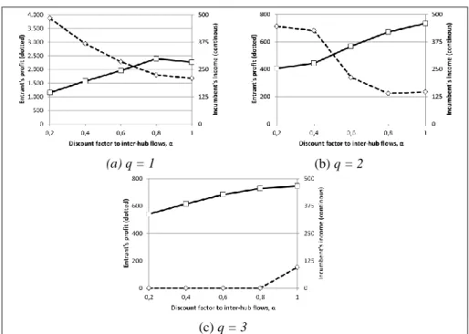
(44) 29. Figure 2-2 shows the results for these three scenarios. The profit earned by the entrant is shown on the left vertical axis of each graph, the income perceived by the incumbent on the right vertical axis, and the inter-hub discount factor (α) on the horizontal axis. We display the incumbent’s income (and not the profit) because the incumbent is supposed to have been in the market for a while, so its investment costs are sunk. Figure 2-2a shows the case in which the incumbent has only one hub located ( q  1 ) and charges a low margin (   0.05 ) over his costs, with customers having an intermediate sensitivity factor (   5.78 ). In this case, for lower interhub costs (lower values of α), the entrant can increase its customer capture and profit by opening more than one hub, taking advantage of the reduced inter-hub costs, which the incumbent, with only one hub, cannot. Figure 2-2b and Figure 2-2c show what happens when q = 2 and q = 3 (the incumbent has two and three open hubs, respectively). Please note the different scale for the entrant profit on these Figures, since now the entrant’s profit is significantly smaller than when q = 1, because the incumbent can take advantage of the inter-hub discounts, achieving a better competitive position and reducing the entrant’s capability of obtaining a higher profit. Figure 2-2c shows how, if the incumbent has a more extensive network, with more than two hubs, it is not convenient for the entrant to start operations in the same market, unless there are no inter-hub economies of scale at all. Our tests show that this situation does not change for different values of Θ. If the leader’s margin Δ increases, the entrant’s profit potentially grows and becomes less dependent on α, even if the incumbent has a larger network with several hubs. Naturally, the incumbent can easily change its margins, making the entrant’s option of competing in this market very risky. The effect of the margin charged by the incumbent on the entrant’s profit is shown in Figure 2-3, for.

(45) 30.   0.6 and   15.39 . The entrant’s profit Z is shown on the vertical axis, while the margin Δ is shown on the horizontal axis. Each series is associated with a different number of incumbent’s hubs, q. Note that the entrant’s profit increases almost linearly on Δ, especially for low values; but not on q. As before, there are situations in which it is not possible for a new competitor to enter the market ( q  5 and small margins, for example).. (a) q = 1. (b) q = 2. (c) q = 3. Figure 2-2. Entrant’s objective function value as a function of α, with Δ=0.05 and Θ = 5.78..

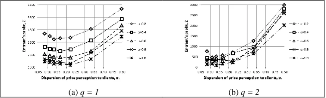
(46) 31. Figure 2-3. The effect of sensitivity to price differences on the entrant’s profit.. Figure 2-4 shows how the entrant’s profit varies as a function of the users’ sensitivity to price differences, Θ. We focus on the case in which the incumbent charges a small margin over its costs (Δ = 0.05), for different values of α. When q = 1 (Figure 2-4a), for high values of Θ, i.e. most of the customers choose the least expensive routes. In other words, there is little spread of customers among the different routes. Since the entrant can locate two or more hubs –taking advantage of inter-hub economies of scale– it can offer routes that are cheaper than those offered by the incumbent, obtaining a reasonable profit. As the value of Θ decreases, more customers are willing to pay higher prices, and the entrant’s advantage due to inter-hub economies of scale, as well as its profit, decreases. However, when customers’ sensitivity to price further decreases, the entrant can increase its prices, obtaining a higher profit. If q = 2, the market is more competitive, because the incumbent is already taking advantage of the inter-hub economies of scale. This is shown in Figure 2-4b. High and intermediate values of Θ put the entrant in a disadvantageous situation, particularly if the incumbent has optimized its hub locations and network. As Θ.

(47) 32. continues decreasing, customers are less sensitive and the entrant can increase its prices and profit.. (a) q = 1. (b) q = 2. Figure 2-4. Entrant’s objective function value as a function of σ, with Δ=0.05, for different values of α.. As intuitively expected, the larger the margin charged by the incumbent, the greater the entrant’s potential profit. Finally, note that curves are not monotonic, and in occasions they intersect each other. This is due to the fact that the genetic algorithm does not guarantee optimality of the solutions obtained.. 2.4.2. Optimal pricing decisions. The pricing problem is decomposable by OD pairs, each pair being an individual market. Every feasible route is a separate product in this market. In this subsection we will not consider the fixed costs of using arcs of the network, to do a fair comparison between both agents. From the entrant’s point of view, there are two possible scenarios: with and without (variable) cost advantage over the incumbent..