Identifying discrete choice models with multiple choice heuristics

Texto completo

(1)PONTIFICIA UNIVERSIDAD CATOLICA DE CHILE ESCUELA DE INGENIERIA. IDENTIFYING DISCRETE CHOICE MODELS WITH MULTIPLE CHOICE HEURISTICS. FELIPE A. GONZALEZ VALDES. Thesis submitted to the Office of Research and Graduate Studies in partial fulfilment of the requirements for the Degree of Doctor in Engineering Sciences Advisor: JUAN DE DIOS ORTUZAR SALAS. Santiago de Chile, June, 2018 Ó 2018, Felipe Antonio González Valdés.

(2)

(3) To all the people who dream of a fairer city. iii.

(4) ACKNOWLEDGMENTS. In first place, I would like to thank everyone that contributed somehow in allowing me to have the opportunity to participate in this program. Thanks Juan Enrique for convincing me to take this step. And to anyone that feels that contributed in my formation, thanks for helping me having the chance to develop myself. Furthermore, I would like to thank who was myself in the past; I do not know if nowadays I would be brave enough to embark in this five years journey. I would like to thank Alejandra, my partner, who has always been there to support me, hold me back, and make me focus on the important things. Thanks to her, I have kept (or even gain) the touch with reality. She has picked me up when I have failed. And probably, the most important thing, she was been my partner throughout this journey. Thanks to my supervisor Juan de Dios. He has always trusted in my capacities and skills, probably overestimating me. I would like to thank him for his attitude, even when he has been collapsed with his duties and overwhelming work load, he always finds time to help me. It has been an honour to work with Juan de Dios. Thanks for guide me to London, where I grew as a person. I would like to thank my friends in the Transport and Logistic Department. Some have been with me since the undergrad and some I have met them in the postgraduate program; to all of them, thanks. Because of you, I have survived an arid research project that at the beginning iv.

(5) of it, the applications where scarce. Thanks to you, I have finished my program with delay, but really enjoying the journey. Special thanks to Sebastián Muñoz, whose friendship was an important support. I thank my parents. To my father who has always guided me through my life. To my mother, whose unconditional support has been key in giving me the confidence to live calmed. To you both, thanks. I would like to thank Ben Heydecker. Thanks for believing in my project and receiving me in London, where I grew in a tremendous way. Moreover, your support and interest in this thesis meant important improvements and developments. Thanks Sebastián Raveau, who has always shown interest in my research and my findings. Thanks to you, this thesis has developed an applied wing. Furthermore, thanks for being a friend with whom I have transited in this journey. Thanks to my thesis committee. The rejection of my upgrade in the first instance allowed me to develop adequately my projects. Thanks for being so responsible in the task you have accepted. To my friends in the student centre. Thanks to you, I developed myself in the program in a sphere that I always dreamed. Thanks VIVE CAI. I would like to thank my out of Transport Department friends. Thanks Toby’s Club for bringing happiness to my journey; you have been there in the darkest hours. To my v.

(6) undergrad friends Catalina and Trinidad, you have always been proud of myself; now also I am. To my friend Concha, who has always overestimated me, at least now I deserve your best thoughts. To the people I met at London and Leeds. Because of you my friends, my stay at the United Kingdom was less hard. I hope to meet you again in life. Thanks to the researchers that have always had a good disposition towards my questions, like Ricardo Alvarez Daziano. Thanks to the researchers that have showed interest in my work, like Stephan Hess, and to David Palma for materializing this interest. Finally, if you feel somehow that contributed in my journey, thanks for being part of it.. vi.

(7) CONTENTS Acknowledgments ............................................................................................................ iv Contents .......................................................................................................................... vii List of tables ................................................................................................................... xiv List of figures .................................................................................................................. xix Resumen ......................................................................................................................... xxi Abstract ........................................................................................................................ xxiv 1.. 2.. Introduction...............................................................................................................1 1.1.. Objectives .................................................................................................................... 4. 1.2.. Hypotheses .................................................................................................................. 5. 1.3.. Methodology ............................................................................................................... 6. 1.4.. Scope of the Thesis ...................................................................................................... 7. 1.5.. Thesis Structure ........................................................................................................... 8. Review and Analysis of Literature ...........................................................................11 2.1.. Methods for Estimating Discrete Choice Models ....................................................... 11. vii.

(8) 2.1.1.. Maximum likelihood estimation ......................................................................... 11. 2.1.2.. Bayesian estimation ........................................................................................... 15. 2.2.. Choice Heuristics ........................................................................................................ 18. 2.2.1.. Random Utility Maximization (RUM) .................................................................. 21. 2.2.2.. Elimination by Aspects (EBA) .............................................................................. 23. 2.2.3.. Random Regret Minimization (RRM) .................................................................. 25. 2.2.4.. Lexicographic behaviour (LEX) ............................................................................ 28. 2.2.5.. Models for dealing with Prospect Theory behaviour ........................................... 29. 2.2.6.. Models of relative evaluation ............................................................................. 31. 2.2.7.. Hard two-step (HTS) heuristics ........................................................................... 33. 2.2.8.. Soft two-step (STS) heuristics ............................................................................. 36. 2.2.9.. Satisficing ........................................................................................................... 37. 2.3.. Techniques for Model Selection................................................................................. 38. 2.3.1.. Hypothesis tests ................................................................................................. 38. 2.3.2.. Information criteria ............................................................................................ 40. 2.3.3.. Out of sample validation .................................................................................... 45. viii.

(9) 2.3.4. 2.4.. 3.. Modelling Multiple Choice Heuristics ........................................................................ 50. Datasets Used in this Thesis ....................................................................................55 3.1.. Las Condes - CBD, San Miguel - CBD dataset .............................................................. 55. 3.1.1.. The dataset ........................................................................................................ 55. 3.1.2.. Creating fictitious choice contexts ...................................................................... 57. 3.2.. 4.. Use of techniques of model selection in this thesis ............................................. 49. Singapore Air Travel ................................................................................................... 60. Further Developments of Choice Heuristics ............................................................63 4.1.. Estimation of the Elimination by Aspects Model ....................................................... 63. 4.1.1.. Estimation of weights in the EBA model ............................................................. 64. 4.1.2.. Estimation of thresholds for continuous attributes ............................................. 73. 4.2.. The Stochastic Satisficing (SS) Choice Model.............................................................. 80. 4.2.1.. On Simon’s theory: principles and motivation .................................................... 84. 4.2.2.. The Stochastic Satisficing model ......................................................................... 87. 4.2.3.. Application to data ........................................................................................... 105. ix.

(10) 5.. 4.2.4.. Conclusions on the Stochastic Satisficing model ............................................... 115. 4.2.5.. Publication history ........................................................................................... 117. Theoretical Analysis of Identifiability of Latent Class Multiple Heuristic Models ..118 5.1.. 6.. Binary Case .............................................................................................................. 119. 5.1.1.. The balance of choice heuristics ....................................................................... 119. 5.1.2.. Examples of balance of heuristics ..................................................................... 126. 5.1.3.. Behavioural diversity of choice heuristics and identifiability ............................. 130. 5.2.. Multiple Heuristics Case........................................................................................... 131. 5.3.. Conclusions on the Theoretical Analysis of Identifiability ........................................ 136. 5.4.. Publication History................................................................................................... 137. Empirical Identification of Choice Heuristics at Sample Level ...............................138 6.1.. Empirical Identifiability of Two Heuristics Models ................................................... 139. 6.1.1.. Experimental design ......................................................................................... 139. 6.1.2.. Analysis of results............................................................................................. 144. 6.2.. Empirical Identifiability of Three Heuristics Model .................................................. 158. x.

(11) 7.. 6.2.1.. Experimental design ......................................................................................... 158. 6.2.2.. Analysis of results............................................................................................. 161. 6.3.. Conclusions of the Analysis of Empirical Identifiability ............................................ 167. 6.4.. Publication History................................................................................................... 169. identifying the Presence of Heterogeneous Discrete Choice Heuristics at an. Individual Level .............................................................................................................170 7.1.. The Mixed Heuristics Model .................................................................................... 172. 7.1.1.. The current approach ....................................................................................... 174. 7.1.2.. The proposed approach and its advantages ...................................................... 174. 7.2.. Testing the Mixed Heuristics Model with Synthetic Data......................................... 176. 7.2.1.. Experimental design ......................................................................................... 176. 7.2.2.. Analysis of results of the synthetic data experiment ......................................... 179. 7.3.. Searching for Heterogeneous Choice Heuristics in an Air Travel Context................. 183. 7.3.1.. Experiment design and estimation ................................................................... 183. 7.3.2.. Analysis of results............................................................................................. 185. 7.4.. Conclusions on the Mixed Heuristics Model ............................................................ 188. xi.

(12) 7.5.. 8.. Publication History................................................................................................... 190. Identification versus Forecasting: Comparing the Performance of Alternative. Multiple HeuristicS Models under Weak and Strong Identifiability ..............................191 8.1.. Experimental Design ................................................................................................ 192. 8.2.. Analysis of Results ................................................................................................... 194. 8.2.1.. Model identifiability ......................................................................................... 194. 8.2.1.. In sample techniques ....................................................................................... 199. 8.2.2.. Out of sample techniques................................................................................. 205. 8.3.. 9.. Conclusions on Identification versus Forecasting..................................................... 211. Conclusions............................................................................................................214. References.....................................................................................................................218 APPENDICES ..................................................................................................................240 Appendix A. Glossary of terms ...................................................................................241. Appendix B. Identification of the EBA model .............................................................242. Appendix C. Detailed results on Singapore travel models..........................................245. xii.

(13) Appendix D. Constants of the experiment of identifiability versus forecasting .........251. xiii.

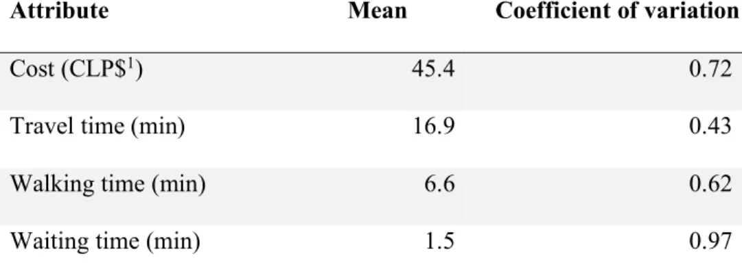
(14) LIST OF TABLES. Table 2-1 Organisation of choice heuristics with explicit choice sets. 20. Table 2-2 Organisation of choice heuristics with implicit choice sets. 20. Table 2-3 Studies reported in the literature using multiple choice heuristics. 53. Table 3-1 Mean and coefficient of variation of the alternative attributes. 56. Table 4-1 Aspects defining alternatives on example of the EBA formula. 64. Table 4-2 EBA weights for each aspect. 71. Table 4-3 Estimation time of EBA model with the analytical and simulation approaches 72 Table 4-4 Initial thresholds for the weight-threshold estimation. 77. Table 4-5 Optimal parameters for the fixed threshold EBA model. 77. Table 4-6 Estimation of thresholds and weights for the EBA model. 78. Table 4-7 Estimation of weights for the optimised thresholds of the EBA model. 78. Table 4-8 Log-likelihood of successive estimations of the EBA model. 79. Table 4-9 Satisficing choice elements, data limitations and simplifications. 90. xiv.

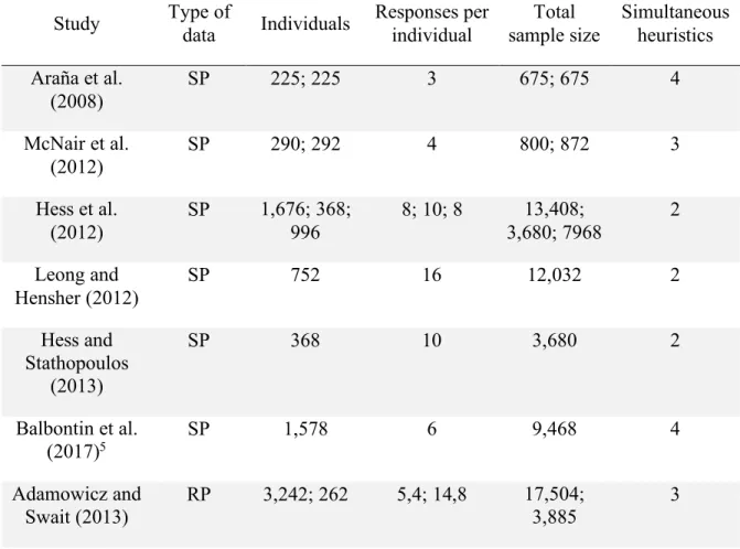
(15) Table 4-10 Parameters used for simulation. 107. Table 4-11 Satisficing and MNL performance in the simulated experiment. 112. Table 4-12 Satisficing model estimation results for real data. 113. Table 4-13 Random utility model estimation results for the real data. 115. Table 5-1 Chosen heuristic and alternatives in the balance examples. 126. Table 5-2 Multiple heuristic model example with strong balance. 127. Table 5-3 Multiple heuristic model example with weak balance. 128. Table 5-4 Multiple heuristic model example with no balance. 129. Table 6-1 Synthetic population latent class parameters. 142. Table 6-2 Choice heuristic simulation parameters. 143. Table 6-3 Identifiability results of RUM and RRM models (number of cases). 147. Table 6-4 Mean and t-test statistic against target value for RUM and RRM models. 149. Table 6-5 Identifiability results of RUM and EBA models. 150. Table 6-6 Mean of RUM parameter estimates and EBA log-weights together with t-test against target values Table 6-7 Identifiability results of RUM and SS models (10,000 DMs) xv. 151 153.

(16) Table 6-8 Identifiability results of RUM and SS models (20 and 40 thousand DMs). 154. Table 6-9 Identifiability results of RUM and SS models with 10,000 DMs and 7 alternatives per choice sets. 156. Table 6-10 Mean and t-test against target values of RUM or SS estimation (10,000 DMs) 157 Table 6-11 Three heuristic class membership function. 160. Table 6-12 Conditional probability of choosing each heuristic in the three heuristics experiment. 160. Table 6-13 Identifiability of the three heuristics case. 161. Table 6-14 Estimation results for RUM in the RUM-EBA-SS model. 163. Table 6-15 Estimation results for EBA in the RUM-EBA-SS model. 165. Table 6-16 Estimation results for SS in the RUM-EBA-SS model. 166. Table 7-1 Heuristic proportions in the simulated experiment. 177. Table 7-2 Simulation parameters for the synthetic population. 178. Table 7-3 LC and HMH success in identifying the chosen heuristic. 180. xvi.

(17) Table 7-4 Average estimation bias for the best MHM case: 5,000 total sample with 25 observations per individual. 182. Table 7-5 Non RUM probability and estimation fit of the LC and MHM models. 186. Table 8-1 Parameters for the 10,000 sample experiment with RRM-SS underlying heuristic 196 Table 8-2 Parameters for the 10,000 sample experiment with RUM-SS underlying heuristic 197 Table 8-3 Parameters for the 20,000 sample experiment with RRM-SS underlying heuristic 198 Table 8-4 Parameters for the 20,000 sample experiment with RUM-SS underlying heuristic 200 Table 8-5 Parameters for the 40,000 sample experiment with RRM-SS underlying heuristic 201 Table 8-6 Parameters for the 40,000 sample experiment with RUM-SS underlying heuristic 202 Table 8-7 Goodness of fit for the ten, twenty and forty thousand sample size experiments 204 Table 8-8 Errors type I and II of the in sample metric studied xvii. 205.

(18) Table 8-9 Cross validation results. 206. Table 8-10 Policies for response analysis. 207. Table 8-11 Likelihood difference of the cross validation and response analysis. 209. Table 8-12 Type I and Type II error probability for each response policy. 210. xviii.

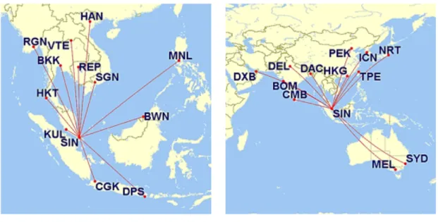
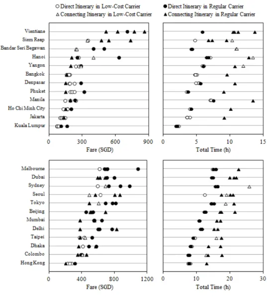
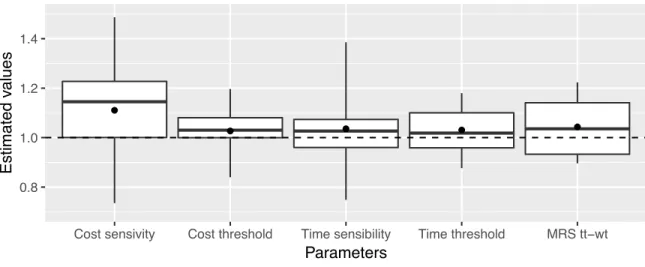
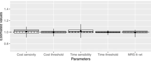
(19) LIST OF FIGURES. Figure 2-1 Trace plot of a Markov Chain. 17. Figure 2-2 Regret function for different scale parameters. 28. Figure 2-3 Classification of out of sample techniques. 46. Figure 2-4 Structure of a latent class model for multiple heuristics. 51. Figure 3-1 Choice set size distribution. 58. Figure 3-2 Trips considered in the Singapore air travel survey. 60. Figure 3-3 Attributes of Singapore air travel survey alternatives. 62. Figure 4-1 Distribution of estimation times for each approach. 73. Figure 4-2 EBA's log-likelihood versus a fictitious threshold. 75. Figure 4-3 Acceptability function versus different scale factors and attribute-threshold differences. 93. Figure 4-4 Indifference curves of two attributes of different acceptability functions. 104. Figure 4-5 Estimated parameters relative to targets in the 500 observations’ sample. 108. Figure 4-6 Estimated parameters relative to targets in the 1,000 observations’ sample. 108. xix.

(20) Figure 4-7 Estimated parameters relative to targets in the 5,000 observations’ sample. 109. Figure 4-8 Alternative specific constants relative to targets in the 500 observations’ sample 110 Figure 4-9 Alternative specific constants relative to targets in the 1,000 observations’ sample 110 Figure 4-10 Alternative specific constants relative to targets in the 5,000 observations’ sample. 111. Figure 6-1 Behavioural difference of RUM and RRM, SS, and EBA. xx. 145.

(21) PONTIFICIA UNIVERSIDAD CATOLICA DE CHILE ESCUELA DE INGENIERIA. IDENTIFICACION DE MODELOS DE ELECCION DISCRETA CONSIDERANDO MECANISMOS DE ELECCION HETEROGENEOS Tesis enviada a la Dirección de Investigación y Postgrado en cumplimiento parcial de los requisitos para el grado de Doctor en Ciencias de la Ingeniería. FELIPE A. GONZALEZ VALDES RESUMEN Entender y predecir el comportamiento de las personas es clave in diferentes áreas, tales como políticas públicas y marketing. Los modelos de elección discreta son una de las herramientas diseñadas para entender estos comportamientos. El núcleo de estos modelos es la heurística de elección; ella representa una forma en que se procesan las alternativas. Su correcto entendimiento es crucial para representar adecuadamente los comportamientos. Numerosas heurísticas se han propuesto en la literatura. Con el objetivo de categorizarlas y entender su relación, hemos creado un marco teórico que las analiza en tres dimensiones: evaluación absoluta/relativa, simplificación de alternativas y simplificación de atributos. De estas heurísticas, hemos seleccionado cuatro para participar en nuestros experimentos: Maximización de la Utilidad Aleatoria (RUM por su nombre en inglés), Minimización del Remordimiento Aleatorio (RRM), Eliminación por Aspectos (EBA) y Satisficing. xxi.

(22) Hemos desarrollado dos contribuciones respecto a Satisficing y EBA. Para Satisficing, construimos el modelo Stochastic Satisficing (SS), que es el primer modelo que implementa completamente la teoría usando datos típicamente disponibles. Para EBA, proponemos un enfoque analítico para acelerar su estimación. Entendiendo que en una población pueden coexistir distintas heurísticas, se han propuesto modelos con múltiples heurísticas. Lamentablemente, su estimación – que usa clases latentes- ha mostrado problemas de identificabilidad. Para entender este problema, hemos estudiado analíticamente la identificabilidad, concluyendo que está gobernada por la diferencia de comportamiento de las heurísticas en la muestra; finalmente, obtuvimos una métrica simple e interpretable para dicha diferencia. Habiendo estudiado la identificabilidad teóricamente, comprobamos sus alcances en la práctica. Estudiamos el impacto de distintas heurísticas, tamaños muestrales y grados de correlación entre los factores que afenta la elección de la heurística y la alternativa. Concluimos que, para nuestro contexto, RRM no es identificable de RUM, SS lo es para muestras grandes (40.000) y EBA siempre es identificable de RUM. Dada la posibilidad de identificar estos modelos, proponemos una metodología que, mediante nuestro Modelo de Heurísticas Mixtas (MHM), facilita la búsqueda de las heurísticas subyacentes y su formulación. El MHM es un modelo de clases latentes con función de pertenencia de clase mixta. Permite encontrar las heurísticas presentes con mayor. xxii.

(23) precisión que el modelo de clases latentes tradicional. Así, sin modelar la función de pertenencia de clase, las heurísticas subyacentes pueden ser encontradas y formuladas. Una vez que modelos candidatos son encontrados, se debe aplicar algún criterio para seleccionar al mejor. Mediante la experimentación con un par de modelos candidatos, concluimos que, si el objetivo es entender el fenómeno, entonces criterios sobre la base de estimación que penalicen débilmente los parámetros adicionales deberían ser usados. Si el objetivo es predecir, entonces se debieran preferir criterios sobre una base de validación. En esta tesis hemos mostrado que es factible estimar modelos con múltiples heurísticas. También, desarrollamos metodologías para encontrar los modelos más explicativos y seleccionar el más útil. Si bien, esta tesis disminuye la dificultad de estimar estos modelos, se requiere más investigación para obtener conclusiones generales. Miembros de la Comisión de Tesis Doctoral. Juan de Dios Ortúzar Salas Luis Ignacio Rizzi Campanella Ricardo Hurtubia González Cristián Angelo Guevara Cue Benjamin G. Heydecker Jorge Vásquez Pinillos. Santiago, Agosto, 2018 xxiii.

(24) PONTIFICIA UNIVERSIDAD CATOLICA DE CHILE ESCUELA DE INGENIERIA. IDENTIFYNG DISCRETE CHOICE MODELS WITH MULTIPLE CHOICE HEURISTICS Thesis submitted to the Office of Research and Graduate Studies in partial fulfilment of the requirements for the Degree of Doctor in Engineering Sciences by FELIPE A. GONZÁLEZ VALDÉS ABSTRACT Understanding and forecasting the behaviour of individuals is key in different realms of society such as public policy and marketing. Discrete choice models are an important econometric tool for understanding these behaviours. The kernel of a discrete choice model is its choice heuristic, which represents the way individuals process the alternatives. A correct representation of their heuristics is key to successfully represent their behaviour. Several heuristics have been proposed in the literature. We have created a framework that allows to organise them and understand their similarity across three dimensions: absolute/relative evaluation, simplification of attributes and simplification of alternatives. We have selected four heuristics for our experiments: Random Utility Maximization (RUM), Random Regret Minimization (RRM), Elimination by Aspects (EBA), and Satisficing. For the last two of these, we made a particular contribution. For Satisficing, we created the xxiv.

(25) Stochastic Satisficing (SS) model, which is the first model that wholly implements satisficing theory using normally available data. For EBA, we proposed an analytical approach to increase its estimation speed. Admitting that not every individual in a population may use the same heuristic, multiple heuristics models have been proposed in the literature. Unfortunately, their estimation using latent classes has given rise to identifiability issues. We studied the problem analytically under a maximum likelihood framework. We concluded that identifiability is closely related with the behavioural differences among the heuristics in the data; we obtained a readily and interpretable measure of this difference. We tested the theoretical findings in a quasi-real transport context. We simulated fictitious individuals choosing real alternatives under our three experimental dimensions. We concluded that, for our context, RRM was non-identifiable from RUM, SS was identifiable from RUM for the larger samples (40.000 individuals), and EBA was always identifiable. Given that it is possible to identify multiple heuristics, we proposed a methodology that, by using our Mixed Heuristics Model (MHM), facilitates finding the heuristics present in a sample and their formulation. The MHM is a latent class model with a mixed class membership function that allows to find the most likely used heuristics with higher accuracy than a non-random latent class model. This way, without modelling the class membership function, the underlying choice heuristics can be found and modelled with a traditional approach. xxv.

(26) Once several models are available, a criterion must be used to select the best one. We tested competing pairs of heuristics with different degree of identifiability. We concluded that if the objective is understanding the underlying phenomena, in-sample criteria that do not penalise heavily additional parameters should be used, promoting more explicative models. Conversely, if the objective is forecasting, out-of-sample validation might be the best approach to promote more robust models. Through our work, we showed that it is feasible to estimate multiple heuristics models. We also provide tools that allow finding the most explicative models and, among them, choose the most useful one. Therefore, after this thesis, the complexity surrounding the use of multiple heuristics models should decrease. Nonetheless, more research is needed to understand the degree of identifiability of these models in different contexts, so that general conclusions regarding the selection of heuristics can be obtained. Members of the Doctoral Thesis Committee: Juan de Dios Ortúzar Luis I. Rizzi Ricardo Hurtubia Cristián A. Guevara Benjamin G. Heydecker Jorge Vásquez. Santiago, August, 2018 xxvi.

(27) 1 1. INTRODUCTION. Understanding and forecasting the decision of individuals is essential in different realms of society. For public policy, for example, it is necessary to value people’s preferences and predict their reaction towards policies affecting their behaviour. Alike, but in the private sphere, in most markets it is important to understand consumers’ choices for designing new products and foresee their reaction towards different companies’ marketing strategies. One of the available techniques for studying people’s preferences and forecasting their behaviour is the use of econometric models. Discrete choice modelling is an econometric tool designed to model the responses of decision makers (DMs) when confronting discrete choice sets. In principle, every output obtained from a discrete set of possible outcomes may be modelled using this tool. These models are particularly useful for representing people’s choices from these sets because of their behavioural interpretation of the individual. Thus, discrete choice models have been widely used to model people’s preferences in different contexts such as the purchase of items (Fader and McAlister, 1990; Adamowicz and Swait, 2013; Beck et al., 2013; Hensher et al., 2013; Palma et al., 2016), housing and location decisions (Martínez et al., 2009; Greene et al., 2017), opinion toward public policy (Araña et al., 2008), and transport mode and route choice (Vovsha, 1997; Ortuzar and Willumsen, 2011). The kernel of an econometric model is its functional form, which is assumed by the analyst to represent the phenomenon. In discrete choice models, the functional form represents a.

(28) 2 choice heuristic, which is a representation of a plausible way of choosing. Initially, only simple behaviours could be correctly modelled –as we detail in Chapter 2– but later, different models have been developed to treat increasingly complex phenomena. Among the complexities faced, one is how to model populations with behaviours of a different nature. Several choice heuristics have been proposed that explains different kind of behaviour. These choice heuristics have been materialized, for example, in the random utility maximization – RUM – model (Lancaster, 1966; McFadden, 1973), the elimination by aspects – EBA – model (Tversky, 1972a, 1972b), and the Satisficing model (Simon, 1955) as the most iconic ones. Another issue is that within a given choice heuristic some decisions may be more complex to model. For example, the popular RUM model’s basic formulation assumes independent and homoscedastic errors and cross-sectional data. More complex versions of this model enables to work with correlated alternatives, panel data, heteroscedasticity, and taste variations (Ortuzar and Willumsen, 2011). A final complexity –that is the target of this thesis– is modelling a population where DMs may use different choice heuristics. In the presence of multiple choice heuristics, a model with a single choice heuristic could misunderstand the phenomenon and fail in prediction. Among the several proposed heuristics in the literature, RUM is the most widely used. Numerous reasons could explain its popularity such as the concordance with classical microeconomic theory, a set of well-developed and desirable properties, and a logical representation of DMs. Despite its popularity, in reality, the high psychological burden.

(29) 3 implied in using RUM in complex decisions could trigger the use of different choice heuristics by DMs. Indeed, behavioural decision theory suggests that the way DMs choose is shaped by the interaction of their cognitive capabilities, personal goals, decision complexities, and the characteristics of the task (Newell and Simon, 1972; Bettman, 1979; Peterson et al., 1979; Denstadli et al., 2012). Therefore, the same context may trigger different heuristics in different DMs. Some attempts have been previously made to model multiple choice heuristics (Araña et al., 2008; Hess et al., 2012; McNair et al., 2012; Adamowicz and Swait, 2013). When trying to characterize the decision of using a choice heuristic, identifiability problems have arisen (Leong and Hensher, 2012b; Hess and Stathopoulos, 2013). All studies found in the literature have tried to model real data, which has given few sparkles about the reason for the non-identifiability problem. This thesis tackles this problem by studying this phenomenon theoretically, by first analytically exploring the properties of the main modelling approach and then, empirically by using a controlled simulated environment given by the choice heuristics, proportions, and variables affecting decisions. Among the several edges of the problem, this study aims to identify whether it is possible to identify different choice heuristics or the conditions that enable such identification. Once identifiability is attained, how to choose the different choice heuristic present in a single model from a wide variety of options is analysed. Finally, we address how to choose a model among several competing ones under weak and strong identifiability estimations..

(30) 4 1.1. Objectives. Our general objective is to study the modelling of a population endowed with multiple choice heuristics. As stated previously, the current state of the art has not been able to properly characterize DMs’ decision processes nor demonstrate the reasons for such a failure. Thus, this thesis intends to give answers to these problems. Given the failure of previous authors to identify explicative models for the selection of choice heuristic, the first main objective is related to the feasibility of identifying such models and may be stated as follows. a) Analyse if it is possible to identify the choice heuristics used by a population and understand the conditions that enable their identification. Given the identification at a population level, several ways to analyse it at an individual level may be proposed which are detailed in this thesis. Then the second main objective is to: b) Analyse if it is possible to identify –probabilistically— the choice heuristics being used by a decision maker. If the first and second objective are accomplished, a useful model that interprets DMs’ behaviour at the population and individual levels will be obtained. Nonetheless, as identifiability issues are frequent, it is possible that several groups of heuristics can interpret the choices with similar fit performance. Therefore, our last main objective is to: c) Analyse which statistical techniques are useful for selecting the most useful model depending of the objective: understand the underlying behaviour or forecast..

(31) 5 For the conclusions to be as general as possible, the findings must be analysed with different sample sizes, number and proportions of choices heuristics, and responses per decision maker.. 1.2. Hypotheses. To study the above main objectives, we will test the following hypotheses: a) It is possible to identify the different choice heuristic used by DMs even if these consider the same attributes. Therefore, identifiability is accomplished just by the different interpretation that heuristics give to alternatives’ attributes. b) For finite sample sizes, the probability of using a heuristic will be recovered – probabilistically and to a reasonable extent—both at the population level and at the individual level. This implies, that the model will be able to identify the probability that each individual has of using each choice heuristic. c) The higher the number of observations per decision maker, the higher the accuracy of the estimation of individual probabilities. d) When models with several choice heuristics are available, in-sample techniques may systematically fail to identify the real underlying model. Conversely, out-of-sample techniques will identify correctly the real choice heuristic..

(32) 6 1.3. Methodology. Given the objectives of the thesis and the hypotheses considered, most of the analyses in this thesis are empirical. Nevertheless, to be able to analyse the results, first a theoretical framework is developed. The theoretical findings enable us to better understand the dynamics of the model and, therefore, adequately interpret the findings obtained in the subsequent empirical experiments. To develop this framework, an analysis of the estimated model is made: we study the optimum first order condition in a maximum likelihood context and the conditions that enable us to obtain a useful covariance matrix. Once the theoretical framework is developed, we test the hypotheses empirically; for this, it is required to have control of the choice heuristics. Therefore, we focus mainly in the use of synthetic populations. A synthetic population creates a testing environment to understand the model’s properties and the impact of the controlled variables in them. Indeed, to test the properties of models in finite samples, the use of synthetic populations is frequently used (e.g. Godoy and Ortuzar, 2008; Raveau et al., 2010; Daly et al., 2012). We vary the experimental conditions and analyse the results of the estimated models under these changes; for example, we consider different sample sizes, choice heuristics and correlation structures. To create the synthetic data, first a fictitious population is created, which behaves according to the desired rules. The fictitious DMs are represented by a set of parameters and available choice heuristics. In each experiment, the set of plausible parameters are based on a real dataset, but modified for the intended purpose..

(33) 7 Once the synthetic population is created, it is given a realistic choice set from which DMs choose. With the objective of having conclusions closely aligned to reality, quasi-real choice sets are used (i.e. real choice scenarios but presented to the fictitious DMs). These choice sets are obtained through random sampling of complete choice sets from a real dataset. Detail about these choice sets are given in Chapter 3. Finally, to show the applicability of the developed methodologies and model’s analysis, existing real dataset are also used. Here, it is not intended to make a deep analysis of the phenomena, but only to show a real application.. 1.4. Scope of the Thesis. The definitions of choice heuristics in the literature do not present important variations, but the limits of what split a heuristic into two different ones is blur. Under our interpretation, certain phenomena that affect the sensitivity of DMs are considered by certain authors as standalone heuristics; we do not differentiate these from the utility maximisation principle and these will not be investigated further. Some authors consider hysteresis and habit as choice heuristics (Adamowicz and Swait, 2013). Other authors consider the phenomenon in which DMs build their preferences along the experiment as a stand-alone heuristic (Hensher and Collins, 2011; Balbontin et al., 2017). Similarly, several choice models have been developed to specifically account for prospect theory (Kahneman and Tversky, 1979). This thesis does not work with prospect theory directly, but makes use of some choice heuristics that could indirectly account for it; the same is the case of modelling certain specific effects.

(34) 8 such as the decoy effect (Fukushi, 2015; Guevara and Fukushi, 2016). In conclusion, all these phenomena are considered within a choice heuristic, rather than standalone mechanisms. Even though we develop several theoretical analyses, this thesis focuses on analysing the multiple-choice heuristics’ problem in an empirical way. Therefore, although the empirical analysis is done as broad as possible in an attempt to obtain the most general conclusions, some of the conclusions attained are not generalizable for every choice dataset. We do not intend to characterise the reason or variables affecting the selection of the choice heuristics of DMs in real experiments. We rather study the model’s capacity to capture these phenomena –if existent at all– and understand the model’s behaviour.. 1.5. Thesis Structure. This thesis starts with an analysis of the literature, which is summarised in the following points: 1. First, we analyse two model estimation methods: maximum likelihood estimation and Bayesian estimation. Advantages of these two methods are explored, and both are used throughout the thesis. 2. We analyse different choice heuristics coming from different fields of study such as transport engineering, marketing, and psychology; in every case the most representative choice heuristics are selected..

(35) 9 3. Techniques for model selection are deeply analysed. We study hypothesis test developed in classical statistics, information criteria coming from information theory, and we end by analysing out of sample validation techniques. 4. Finally, we discuss the experience reported in the literature regarding the modelling of multiple choice heuristics. We use two datasets in this thesis. With the aim of not having to describe them in each chapter, we analyse them in Chapter 3. Moreover, we detail there the way the datasets are used to create pseudo-synthetic scenarios. After the literature analysis, we identified potential contributions regarding two heuristics. Therefore, in Chapter 4 we further developed an important contribution regarding the Satisficing heuristic (Simon, 1955) and a smaller one in relation to the Elimination by Aspects heuristics (Tversky, 1972a, 1972b). In Chapter 5, we conduct the theoretical analysis of the multiple heuristics model. First, we analyse a binary case that helps to enlighten the underlying phenomena; later we generalise it to the multivariate case. In both cases, we start by analysing the optimum first order conditions on the likelihood function. Then, we explore the second order conditions and their relationship to the covariance matrix. In Chapter 6, we start the empirical analysis of multiple heuristics in this thesis. We analyse the identifiability of a latent class multiple heuristics model at the population level. Here we explore several dimensions that may affect model identifiability. Within a two heuristics.

(36) 10 model we analyse the type of choice heuristics involved in the model, sample size, number of alternatives in the choice set, and the proportion of each heuristic in the sample. We end this chapter by analysing a three heuristics case. Chapter 7 is based on the findings of the previous chapter. Here, we analyse the identifiability of those heuristics where identifiability was more probable at an individual level. We finally apply the findings to a real sample. In Chapter 8, we attain our last objective: we analyse the case where different pairs of heuristics can represent the same in-sample behaviour. We analyse in sample and out of sample indicators in cases where weak and strong identifiability is achieved and discuss their use. Finally, conclusions of this thesis are addressed in Chapter 9. We analyse the main findings and its implications for choice modelling. We also discuss the limitations of this study and how it may affect the results. We hypothesise about the impact of the variation on the imposed experimental conditions. Finally, we end by addressing different avenues that this thesis has opened for future research..

(37) 11 2. REVIEW AND ANALYSIS OF LITERATURE. In this chapter we analyse three main topics. First, estimation techniques, particularly those used in this thesis (maximum likelihood estimation and Bayesian estimation). Then, we describe several choice heuristics and organise them in a form suitable for discussion. Finally, we study techniques for model selection.. 2.1. Methods for Estimating Discrete Choice Models. In this thesis, we attempt to estimate models of which identification is not guaranteed; therefore, the estimation technique chosen must consider this issue. We examine two estimation techniques: maximum likelihood estimation, which is the most popular alternative in transport engineering, and Bayesian estimation, which is interesting because there is no maximization problem involved. Both are explained as follows.. 2.1.1. Maximum likelihood estimation. In maximum likelihood estimation, we assume that the vector of outputs 𝑥 and model parameters 𝜃 have a joint density function 𝑓(𝑥, 𝜃) given by (2.1). In it, 𝑓 represents the model. Pr(𝑥, 𝜃) = 𝑓(𝑥, 𝜃). (2.1).

(38) 12 The likelihood function measures the plausibility that the parameter 𝜃 of a model acquires a certain value in light of the data (2.2). ℒ (𝜃|𝑥) = 𝑓(𝑥|𝜃 ) = Pr(𝑥|𝜃). (2.2). Specifically, the likelihood function describes the probability of occurrence of the observed outcome 𝑥 conditional on a model structure and model parameters 𝜃. The maximum likelihood estimation tries to find the model parameters that maximise the observed outcome (2.2). If all 𝑖 observations are independent, then (2.2) is reduced to (2.3).. ℒ (𝜃|𝑥) = - Pr(𝑥. |𝜃). (2.3). .. Given that the multiplied term in (2.3) is a probability –which ∈ [0,1]– and that usually many DMs are considered, it is numerically hard to maximise (2.3) due to its small magnitude. Then, the expression maximised is the logarithm of the likelihood or log-likelihood given by (2.4).. 𝑙(𝜃|𝑥) = 6 log(𝑃𝑟(𝑥|𝜃 )). (2.4). .. If the model is correctly specified, the model parameters distribute asymptotically Normal (Ortuzar and Willumsen, chap. 8, 2011; Train, chap. 8, 2009), as in: >. 𝛽= → 𝑁(𝛽, −𝑯CD ). (2.5).

(39) 13 In (2.5), 𝑯 represent the hessian matrix of the log-likelihood function as stated in (2.6). The negative of H is also called the information matrix (Ortuzar and Willumsen, 2011, chap. 7; Train, 2009, chap. 8). When the model is not correctly specified the Hessian matrix in (2.6) is replaced by the robust Hessian matrix (Train, 2009, chap. 8).. 𝑯=. 𝜕 F 𝑙 (𝜃 ) 𝜕𝜃 F. (2.6). Frequently, the maximum likelihood can hardly be calculated analytically and numerical maximisation is needed. This kind of optimisation is suitable for single heuristic models, like those in Chapter 4. Unfortunately, it can pose a problem for weakly identifiable models, as those being characterised in Chapters 5 to 8. Throughout this thesis, we assess the degree of identifiability of the models. In maximum likelihood, non-identifiability is detected by means of a non-invertible hessian or negative standard deviation estimates. However, there are several reasons that could explain these phenomena: i) poor asymptotic behaviour of the estimates (2.5), ii) numerical approximation algorithms are not at the optimal point, and iii) the model is, indeed, non-identifiable. Even though the first two problems can be tackled, they are non-dismissible. To estimate the models via maximum likelihood, the R software (R Core Team, 2016) with the Maxlik package (Henningsen and Toomet, 2011) are used in this research. In the Maxlik package –as well as in other packages–, all the optimisers calculate the robust hessian matrix. Most of the available optimization methods are algorithms that work on a continuous space.

(40) 14 solution; while one of the methods, Simulation Annealing, works in a non-continuous space solution. The algorithms for non-continuous space optimisation are normally not suitable for maximum likelihood estimation. Preliminary simulations performed by us indicate that although Simulation Annealing fails in finding the optima, the solutions provided are acceptable. Two problems with this algorithm are that the “optimal point” identified changes from estimation to estimation and, because the point is suboptimal, the hessian matrix may be non-invertible. The latter problem implies an impossibility of obtaining a covariance matrix for the estimates. Yet, if the space of the likelihood is non-continuous, like in the estimation of thresholds in an Elimination by Aspects model, the only available method in this package is Simulation Annealing. The algorithms for continuous space optimisation are normally more suitable than noncontinuous space algorithms. However, they tend to be captured in local optima, which is a frequent phenomenon in latent class models, which are the main models used in this thesis. Then, maximum likelihood poses two problems in the context studied in this thesis. First, the impossibility of the inversion of the hessian matrix or the presence of negative standard deviation estimates cannot be uniquely linked to the non-identifiability of the model as a cause. And second, the most suitable algorithms for maximum likelihood tend to be captured by local optima. Therefore, an alternative estimation procedure is considered as an option for multiple heuristic models..

(41) 15 2.1.2. Bayesian estimation. Bayesian estimation identifies the most probable distribution of the parameters or posterior distribution in light of the data given a distribution of plausible values or prior. It is based on the Bayes theorem expressed in (2.7).. Pr(𝜃|𝑦) =. Pr(𝜃) Pr(𝑦|𝜃 ) Pr (𝑦). (2.7). The first component Pr(𝜃) is a probability distribution of the parameters; its density function incorporates all available knowledge or prior belief. The second element Pr(𝑦|𝜃 ) is the likelihood function, as stated in (2.2), which relates the probability of generating the data under the model and parameters. The last component Pr (𝑦) is the data density and is usually omitted since the model can be calculated with (2.8). Pr(𝜃|𝑦) ∝ Pr(𝜃) Pr(𝑦|𝜃). (2.8). Despite the existence of simple cases where the convolution of the likelihood and the prior have a closed form –in this case known as conjugate prior–, in most cases (2.8) cannot be calculated analytically (Gelman et al., 2013, cap. 12). Normally, to obtain useful statistics such as mean and variance or the empirical shape of the posterior, numerical integration is needed. Several techniques for calculating this convolution exists, such as gridapproximation, maximum a posteriori, and Markov Chain Monte Carlo (McElreath, 2012). The latter is the most general technique and is the one used in this thesis..

(42) 16 Markov Chain Monte Carlo (MCMC) is a stochastic method for numerical integration (Gelman et al., 2013). This technique samples from the desired distribution (Pr(𝜃|𝑦)) to obtain an approximation of the parameter distribution. There are several algorithms that implement MCMC, such as Metropolis Hastings, Hamiltonian sampling, and Gibbs sampling. In this thesis, we use Gibbs sampling1 as implemented in the JAGS software (Plummer, 2003) connected to R through the RJags package (Plummer, 2016). Gibbs sampling sequentially samples one parameter of the model conditional on the last values sampled for rest of the parameters (Gelman et al., chap. 11, 2013). Therefore, the parameter distribution depends exclusively on the current value of the rest of the parameters and not upon its history; hence, the sequence of sampled parameters is a Markov chain. The sampler sequentially obtains observations for each parameter of the model until the desired number of iterations or convergence is reached. For the Gibbs sampler –or any other sampler–to be able to approximate (2.7), the Markov chain must be in a stationary state. Depending on the structure of the Markov chain and the initial points, different iterations must be performed before the chain reaches a high joint density function point, which is usually named burn-out period (Godoy and Ortuzar, 2008).. 1. We also tested the STAN software (Stan Development Team, 2015) that implements Hamiltonian sampling.. For simple probability functions, STAN is faster than JAGS; however, if every individual has a structurally different probability function, like in the EBA model, the compilation time can be extremely large..

(43) 17 Once the parameters are in the high density function point, all sampled values may be used (Kass et al., 1998). To analyse convergence, several tools may be used. Even though semi-automatic tools exist, the manual inspection of the Markov chains is recommended (Lunn et al., 2012). Convergence is analysed using a trace plot of the estimates and a density graph of the parameters. The trace plot of a parameter shows the value sampled for it in each iteration. Two examples are presented in Figure 2-1. Figure 2-1 Trace plot of a Markov Chain. The trace plot is useful to determine whether the estimates of the Markov chain are stable in mean and variance. The left panel represents a parameter that does not have a stable mean; whereas the right panel shows parameter with stable mean and variance. A stable variance is represented by a non-varying dispersion of the trace plot. Shocks within the trace plot are expected, since low density events should be also represented, but no tendency should be obtained. The density graph of the parameters plots the approximate density function obtained by sampling. Given the structure simulated in this thesis with unique underlying “real”.

(44) 18 parameters in each simulation, we expect a soft and unimodal density function (i.e. with only one peak). If the density function is not soft, then more sampling is needed. If the density function is not unimodal, then the Markov chain has not reached convergence or has a mixture of convergence and non-convergence sampling.. 2.2. Choice Heuristics. The kernel of a discrete choice model is its choice heuristic, that is the procedure that DMs are supposed to follow to choose an alternative from a choice set. In other words, the choice heuristic is the set of rules that links certain sensitivities or parameters to a specific choice. To represent different behaviours, different heuristics have been proposed in the literature. Indeed, some heuristics try to represent a specific psychological theory (Simon, 1955; Kahneman and Tversky, 1979), while others represent different degrees of rationality (Chorus et al., 2008; McFadden, 1973). In the literature, the terms of heuristic and choice model have been used normally as equivalent terms. Even though this is correct when a single heuristic exists, when multiple heuristics are embedded in the same model, a distinction is needed. In this thesis, and consistent with some literature (e.g. Cantillo and Ortúzar, 2005; Kivetz et al., 2004), the heuristic will be taken as the specific set of rules or mechanisms that DMs follow to choose, while the model, is a mathematical representation of one or more choice heuristics..

(45) 19 We analyse several choice heuristics that have been proposed and organise them using three criteria. Even though not all choice heuristics present in the literature are analysed, an extensive number of them is considered. The first criterion is whether the choice heuristic evaluates alternatives in a comparative (relative evaluation) or in an absolute (absolute evaluation) fashion. Heuristics in the former group are contextually dependant and generally try to apply some concepts of Prospect theory (Tversky and Kahneman, 1991). Heuristics in the latter group are economically rational and exhibit the property of independence of irrelevant alternatives. The second criterion analyses if all alternatives’ attributes are evaluated (total evaluation) or if only a subset of them (limited evaluation) is considered. Heuristics in the limited evaluation cluster implement strategies that operate in contexts where a total evaluation strategy would involve high cognitive burden due to the number of attributes involved. The last criterion is designed to verify if the individual chooses applying several processes or a single straightforward one. Implicit choice set heuristics or two-stage heuristics first reduce the size of the choice set (i.e. screens alternatives) and later chooses with an explicit choice set heuristic. An explicit choice set heuristic selects an alternative from the choice set using a single procedure. Moreover, even though any explicit choice set heuristic can be transformed into an implicit choice set heuristic by adding a screening stage, to the best of our knowledge, no relative evaluation two-stage choice heuristic has been proposed. The choice heuristics presented are organised according to these criteria in Tables 2-1 and 2-2. These tables enable to visualise the kind and degree of similarity between the analysed.

(46) 20 heuristics and, furthermore, offer a framework to analyse/organise other choice heuristics. This framework allows us to select a subset of choice heuristics to test in the experiments. Table 2-1 Organisation of choice heuristics with explicit choice sets. Explicit choice set. Total evaluation. Limited evaluation. Absolute. EBA RUM. evaluation. LEX RAM LA. MCD. RUM-RRM Relative. RRM. evaluation. CC. Table 2-2 Organisation of choice heuristics with implicit choice sets Implicit choice set. Absolute evaluation. Relative evaluation. Total evaluation. STS. Limited evaluation. HTS. Satisficing.

(47) 21 Finally, the following conventions will be used in this thesis. First, the modeller will be referred to as female, and the decision makers as males. Second, because the choice heuristics come from different bodies of knowledge (e.g. marketing, psychology, statistics and engineering), the nomenclature used is not straightforward and is stated in Appendix A.. 2.2.1. Random Utility Maximization (RUM). Random Utility Maximization (RUM) is a choice heuristic where DMs choose the alternative that maximise their utility. The utility of a given alternative 𝑖 for individual 𝑞 (𝑈K. ) is a construct used by individuals to summarise all the characteristics of an alternative into a single figure of merit. When applied, the utility maximization problem (or consumer problem) is solved and an indirect utility function is obtained, which is usually the expression estimated (for further details see McFadden,1981). The modeller assumes that there is a part of the utility that she can identify (𝑉K. ) –which is frequently linear and additive in parameters– while the other part is considered a stochastic error (𝜖K. ) as in (2.9). 𝑈K. = 𝑉K. + 𝜖K.. (2.9). Depending on the distribution of the error terms, the model obtained varies. A Normal error term generates a Probit model (Daganzo, 1979). Independent and identical distributed Gumbel errors generate the Multinomial Logit (MNL) model (McFadden, 1973), which has been for many years the most popular formulation (2.10):.

(48) 22 𝜖. ~𝐺𝑢𝑚𝑏𝑒𝑙(0, 𝜎 F ) 𝑃K. = 𝜆=. exp (𝜆 · 𝑉K. ) ∑\∈] exp (𝜆 · 𝑉K\ ). (2.10). 𝜋 𝜎√6. Because the MNL model has several assumptions that are easily violated (e.g. homoscedasticity and independence of observations and errors), several alternative models have been proposed. A more flexible generalisation of the MNL, the nested logit (Williams, 1977; Daly and Zachary, 1978), works with partially correlated alternatives. A further but less popular improvement is the cross-correlated or cross-nested logit (Vovsha, 1997; Bhat, 1998; Ben-Akiva and Bierlaire, 1999). Furthermore, computing development has enabled the estimation of even more flexible models like the mixed logit model (Cardell and Reddy, 1977; Train, 1998). The mixed logit model enables a general covariance structure (Train, 2009) and can approximate any discrete choice model derived from RUM as closely as one pleases (McFadden and Train, 2000). Developments over the MNL model have not only addressed the error term. Modifications of the MNL’s utility function have been applied also, for example to create the dogit model (Gaundry and Dagenais, 1979), which allows to handle captives users. Further improvements in the modelling of non-measurable (latent) variables have been also some important developments (Ben-Akiva et al., 2002, 2012; Raveau et al., 2010). Finally, latest development of the RUM heuristic allows to model DMs considering the simultaneous.

(49) 23 decision of choosing a discrete alternative and, conditional on it, evaluate a continuous consumption level (Bhat, 2005, 2008; Pinjari and Bhat, 2010; Calastri et al., 2017b, 2017a). Even though the MNL model requires strong assumptions, given that it is the most popular and simple model, it is the one used that will be used in this thesis. Thus, from now on the MNL model and the RUM choice heuristic will be used unequivocally.. 2.2.2. Elimination by Aspects (EBA). Elimination by Aspects –EBA– (Tversky, 1972b, 1972a) is a choice heuristic applicable in complex situations where DMs face an overwhelming amount of information. EBA is a nonindependent random utility model (Tversky, 1972a) that sequentially discards alternatives based on their attributes. Even though in its general form the EBA is able to model a diversity of situations, having as special cases the MNL, the Nested Logit model, and the Cross Nested Logit model (Kohli and Jedidi, 2015, 2017; Aribarg et al., 2017), in this thesis we consider that heuristics derived from random utility theory as stand-alone heuristics differ from EBA. In EBA, alternatives are completely described by aspects, defined as discrete desirable2 characteristics that are directly mapped from the alternative’s attributes. If the attribute associated to an aspect is discrete, then, a discrete set of aspects directly describes the attributes. However, if the attribute is continuous, there is no straightforward representation. 2. Tversky (1972b) postulates that an alternative model could consider an heuristic with undesirable attributes. where regret is involved. However, this formulation is out of the scope of this thesis..

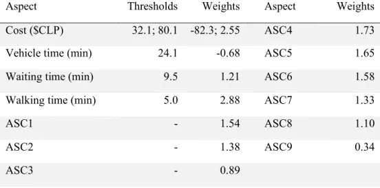
(50) 24 of the aspects. The most common representation considers a threshold that divides the attribute into acceptable (or desirable) and unacceptable (or undesirable). Unfortunately, the methods to estimate such threshold are scarce and are further addressed in Section 4.1. In the EBA heuristic, DMs are supposed to choose an aspect from the set of available aspects and eliminate all alternatives that do not have the it. The process continues until only one alternative is available, which is then chosen. The inspection order, or ranking of aspects, could be deterministically determined for the individual. However, to accommodate different decision profiles and uncertainty, the modeller assumes that DMs choose stochastically the inspected attribute. Therefore, the stochastic nature of the model lies in the stochasticity associated with the inspection order. The aspects are the only elements involved in the decision process. The importance of each aspect is given by a positive continuous variable 𝑤 ∈ 𝑊 named weight, that is positively correlated with the probability of choosing the aspect. The most common formulation of EBA selects one aspect with a probability proportional to the weight of the available aspects in the current choice set (2.11). To freely3 estimate the weight (i.e. unconstrained in ℝ), the log-weight (𝛼) is normally estimated as in (2.12).. 3. This is needed in maximum likelihood estimation since the estimators distribute asymptotic Normal.. Additionally, it is desirable in Bayesian estimation in order to have a higher variety of priors available..

(51) 25 𝑃. =. 𝑤. ∑∀\ ∈ fgf.hfihjk 𝑤\. wm = exp(𝛼n ). (2.11). (2.12). Different formulations of the aspects and the probability of selecting them generate different types of EBA models. The Hierarchical EBA heuristic, or PRETREE, is used to model the selection of aspects that are not independent (Tversky and Sattath, 1979). The Elimination by Dimensions heuristic (Gensch and Ghose, 1992) and Elimination by Cut-offs (Manrai and Sinha, 1989) try to tackle the problem of EBA’s thresholds on continuous attributes. Even though the EBA can accommodate several behaviours, only the most common version –and the most popular one– will be used (2.11) here and will be identified unequivocally as EBA.. 2.2.3. Random Regret Minimization (RRM). Random Regret Minimization –RRM– (Chorus et al., 2008) is a heuristic where DMs value alternatives relatively. It is based on the concept of anticipated regret, that is, the feeling triggered when the individual imagines how would have been the situation if he had taken another choice (Simonson, 1992). Indeed, the relationship between the anticipated regret and choice is a well-studied problem in psychology (e.g. Zeelenberg, 1999; Zeelenberg and Pieters, 2007)..

(52) 26 The first formulation of the RRM model (2.13) is a direct interpretation of the economic principle of minimising the maximum loss (Savage, 1951). If the error term is Gumbel distributed, the model adopts the logit model structure (2.14). min 𝑅. = min max 𝑅.\ + 𝜖. .. .. .t\. (2.13) = min max u6 𝑚𝑎𝑥 w0, 𝛽x y𝑥\x − 𝑥.x z{| + 𝜖. .. .t\. x. 𝑃. =. exp (−𝜆𝑅. ) ∑∀\∈} exp (−𝜆𝑅\ ). (2.14). Even though (2.13) exhibits a simple structure, model estimation is not straightforward due to the 𝑚𝑎𝑥 operator. Then, typically an approximate function is used (Chorus, 2010), which is shown in (2.15). This is the most popular version of the RRM model, also known as RRlog (Jang et al., 2017).. 𝑅. ≈ 6 6 ln w1 + 𝑒𝑥𝑝 w𝛽x y𝑥\x − 𝑥.x z{{ ∀\∈}t. ∀n∈€. (2.15). Several other versions of the RRM model have been proposed, one of them, the µ-RRM (van Cranenburgh et al., 2015), enables to further exploit the flexibility of the model (2.16). The RRlog model is not scale-invariant; hence, the scale may be estimated. The µ-RRM exploits such feature and estimates the scale at the expense of additional parameters. Even though, several other random regret models have been proposed, such as the generalized-random regret model (Chorus, 2014) or the pure-random regret model (van Cranenburgh et al., 2015), they will not be further analysed since they do not represent a significant –or any–.

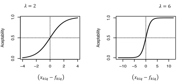
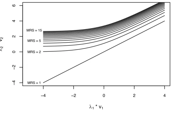
(53) 27 improvement over the µ-RRM model and only enable further understanding of the regret function.. 𝑅. ≈ 6 6 𝜇x ln ‚1 + 𝑒𝑥𝑝 ƒ ∀\∈}t. ∀n∈€. 𝛽x y𝑥 − 𝑥.x z„… 𝜇x \x. (2.16). The µ-RRM has two variables per attribute-regret function which allows to change the degree of regret associated to each attribute. The 𝜇 parameter controls the shape of the regret and the 𝛽 parameter controls its magnitude. The behaviour of the 𝜇 parameter is shown in Figure 2-2. The blue line represents the traditional RRM model. The red lines, for which the shape parameter is indicated, represent the two most extreme cases where the 𝜇 parameter takes the higher and smaller values. For high values, the 𝜇-RRM model exhibit a behaviour where the penalisation of the losses compared to the gains is not extreme (in the RUM model the penalisation is null). On the other hand, for small values the model exhibits a high profundity of regret (van Cranenburgh et al., 2015), where the penalisation of the losses are extreme and the valuation of the gains are non-existent. Finally, the black line denotes an intermediate behaviour between the higher value of the shape parameter and RRM..

(54) 28. 6 4. mu = 2.5. 2. Regret. 8. 10. Figure 2-2 Regret function for different scale parameters. 0. mu = 0.1 −15. −10. −5. 0. 5. 10. 15. Regretted attribute. The RRM has become popular in several domains. Applications are mainly found in transport, dealing with route choice (Leong and Hensher, 2012a; Chorus and Bierlaire, 2013), vehicle purchase (Beck et al., 2013), searching of parking space (van Cranenburgh et al., 2015), manoeuvre in car accidents (Kaplan and Prato, 2012), and transport mode (Chorus, 2010). Other applications can be found in health economics (Boeri et al., 2013) and marketing, to analyse online dating (Chorus and Rose, 2012).. 2.2.4. Lexicographic behaviour (LEX). A Lexicographic choice heuristic privileges a single attribute over the rest. Only when the differences over the sought attribute are not noticeable, another attribute may be considered (Tversky, 1969). It has been argued that complex choices could trigger this choice heuristic (Ortuzar and Willumsen, 2011), and it has even been reported in simple decision tasks (Tversky et al., 1988). This choice heuristic has the particularity that no utility function can.

(55) 29 accommodate it (Debreu, 1954) and in some specific context it can outperform compensatory structures (e.g. Jedidi and Kohli, 2008). The LEX choice heuristic is not intended to model all choice situations, thus, applications are not extensive. Moreover, distinguishing lexicographic behaviour from compensatory structures is not straightforward, since the response pattern of LEX could also be formed by compensatory responses (Saelensminde, 2006). It can be argued that a lexicographic behaviour is a reduced version of an EBA heuristic. The EBA heuristic categorises alternatives into desirable aspects, therefore, if the only sought aspect is if the alternative has the best value of the analysed attribute, then, EBA is consistent with lexicographic behaviour. Hence, LEX may be interpreted as an extreme version of the EBA heuristic. Thus, only EBA will be used for experimentation in this thesis.. 2.2.5. Models for dealing with Prospect Theory behaviour. Prospect theory departs from the classic rational economical behaviour by anchoring in three key elements: (i) preferences are context-dependent, (ii) losses loom larger than gains, and (iii) DMs may perceive biased probabilities. The theory assumes that although DMs are utility maximisers, they perceive attributes subjectively. In sections 1.4 and 2.2 we have defined the limits of a choice heuristic. Prospect theory heuristics are in the blur limit between being contained in the RUM paradigm and being stand-alone. Although we consider that DMs following prospect theory behaviour are still utility maximisers, we consider this separately given its importance..

(56) 30 There are a family of models that try to capture the principles of Prospect theory (Kahneman and Tversky, 1979). Among the concepts applied, we describe the ones that focus on loss aversion (i.e. gains are valued different than losses). Gains and losses are compared against a reference; different reference points and utility functions gives birth to different models. Most of these models keep the RUM structure; indeed, they could be interpreted as RUM models with a different utility function. However, they are analysed as a different choice heuristic since they value alternatives relative to a reference point.. 2.2.5.1.. Loss Aversion (LA). The loss aversion heuristic (Tversky and Kahneman, 1991) values gains differently than losses compared to the statuo quo. The utility function is piece-wise defined linear and additive (2.17):. 𝑉. = 𝛽† + 6 ‡ x. 𝛽x (𝑥.x − ‰‰‰‰‰), 𝑥ˆx (𝛽x + 𝜆x )(𝑥.x − ‰‰‰‰‰), 𝑥ˆx. 𝑥.x ≥ 𝑥\x 𝑥.x < 𝑥\x. (2.17). In (2.17), one branch represents the gain domain and the other the loss domain. If the attribute is desirable, the first branch represents gains with respect to the status quo valued at a 𝛽x rate; whereas, the other branch, represents the loss domain that is penalised higher through the loss aversion parameter (𝜆x ). If the attribute is undesirable the relationship is inverse..

(57) 31 In the LA model, the relationship between the RUM heuristic and Prospect Theory is evident: the latter provides further insights about the way that DMs value attributes, but do not challenge the principle of utility maximisation.. 2.2.5.2.. Contextual Concavity (CC). The CC heuristic (Kivetz et al., 2004) implements the concept of context dependence and loss aversion. It values each attribute against the best one available in the choice set (2.18). Ž•. 𝑈. = 𝛽† + 6 ‚𝛽n Œ𝑥.x − max 𝑥\x •… x. \. + 𝜖.. (2.18). In (2.18) the 𝜙 parameter generates a concavity or convexity in the utility function depending of its value. When the model is concave, i.e. 𝜙 ∈ (0,1), losses are valued more than gains. The max operator induces context dependence and positions the concavity point. Again, as in the LA model, the relationship between RUM and Prospect Theory is evident.. 2.2.6. Models of relative evaluation. The objective of the following heuristics is to evaluate alternatives relatively. DMs build a representation of the alternative based on the alternative performance compared to other alternatives. The individual evaluates the ratio of gains and losses of the various alternatives considered. Among several formulations that model this feature, there are two that have been recently tested in transport research: the Relative Advantage Maximisation model and the Majority of Confirming Dimensions model..

(58) 32 2.2.6.1.. Relative Advantage Maximisation (RAM). RAM (Tversky and Simonson, 1993) attempts to value context independent and context dependent features into a single unit of merit (2.19). Context independent features are modelled as a RUM-like structures (𝑉. ), whereas context dependent features are modelled as a relative measure of advantage (𝐴x ) and disadvantages (𝐷x ) over other options (2.20). 𝑈. = 𝛽g 𝑉. + 𝛽“ 𝑅.} + 𝜖.. 𝑅.} = 6 𝑅.\ = 6 6 ∀\ t.. ∀\ t. x. 𝐴x (𝑖, 𝑗) 𝐴x (𝑖, 𝑗) + 𝐷x (𝑖, 𝑗). (2.19). (2.20). Equation (2.20) indicates how the relative performance of an alternative is linked to relative advantages and disadvantages. Tversky and Simonson (1993) suggests defining advantages and disadvantages asymmetrically, so that disadvantages are more valued than advantages. Even though this definition aligns with Prospect Theory (Kahneman and Tversky, 1979), no statistical evidence supports such proposal for this particular model yet (Kivetz et al., 2004). Finally, Equation (2.21) indicates the relationship between the attributes of the compared alternatives and the corresponding advantage: 𝛽 (𝑥 − 𝑥\x ), 𝐴x (𝑖, 𝑗) = • n .x 0,. 𝛽x (𝑥.x − 𝑥\x ) > 𝜏 x 𝑜𝑡ℎ𝑒𝑟 𝑐𝑎𝑠𝑒. (2.21). Specifically, 𝛽n values a desirable difference of an attribute of the selected alternative (𝑖) compared to another one (𝑗). The variable 𝜏 corresponds to a minimum perception threshold..