Chapter II
Hypothesis testing
…...
..
…...
Objetive
Chapter
Developing the methodology of
hypothesis testing to analyze
differences and make decisions,
determine the risks involved in
making such decisions if we rely
solely on information from the
probability sample, and
the
2.1 Introducción
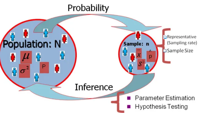
Inferential statistical methods are a way to extract conclusions about a population, the data obtained from a probability sample. Statistical Inference involves two main types of techniques: Parameter Estimation and Hypothesis Testing. Whatever the technique used, the overall purpose is to use data from a probability sample to extract conclusions about a population.
Hypothesis testing is very important in the scientific community and is necessary for advancing theories and ideas. Hypothesis tests are very useful and application in economics. An important component of the total quality management (TQM) is the use of Statistics and Statistical thinking in continuous improvement and in decision making. As Businesses have recognized the importance of Statistics, they have increasingly questioned the statistical education of business school graduates. Statistics play a vital role in a wide variety of business decisions today, from planning and interpreting market research and economic data to developing work volume forecasts.
The following figure 2.1 shows the process of inferential statistics:
Figure 2.1 Process of inferential statistics
2.2 Hypothesis Test
A statistical hypothesis is an assumption on one or more populations that may be true or not. The statistical hypotheses can be compared with information extracted from the samples and whether they are accepted as if rejected can make a mistake. Since in practice not know if the decision is correct or not, we must choose contrasts that minimize the probability of error of type I and II. However, this is not possible because these probabilities are complementary sense, as when one increases the other decreases. Therefore, the criterion used is to set the significance level, choosing from all tests (statistical tests) possible, with a significance level that makes possible the risk or, which is, maximizes the power.
Purpose of hypothesis testing
The purpose of hypothesis testing is to determine whether there is enough statistical evidence in favor of a certain belief about a parameter.
Example: Is there statistical evidence in a random sample of potential customers that support the hypothesis that more than 10% of the potential customers will buy a new product?
The assumption made with intent to reject the null hypothesis is called and is denoted by Ho. Reject Ho implies accepting an alternative hypothesis (Ha).
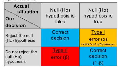
Two types of errors may occur when deciding whether to reject H0 based on the statistic value.
Type I error ( ): Reject the null (Ho) hypothesis when it is true. Type II error ( ): Do not reject the null (H0) when it is false.
Realize, that a small p-value (or observed level of significance) suggests that the alternative hypothesis is true, but does not guarantee it is true.
Actual
situation
Our
decision
Null (Ho)
hypothesis is
false
Null (Ho)
hypothesis is
true
Reject the null (Ho) hypothesis
Correct
decision
Type I
error (α)
Called Level of Significance
Do not reject the null (Ho) hypothesis
Type II
error (β)
Correct
decision
(1-β)
Figure 2.2. Error Type
Note: do not reject the null hypothesis or Fail to Reject null hypothesis
Details to note:
and are inversely related.
Only both can be decreased by increasing the sample size "n".
Steps in Hypothesis Testing
1. Making Assumptions and Meeting Test Requirements Model: Random sampling
Level of measurement is interval-ratio
Sampling distribution is normal (we can be sure that this assumption is satisfied by using large samples. (Central Limit Theorem)
Specify the population value of interest
If you have two or more groups check assumption about homogeneity 2. Formulate the appropriate null and alternative hypothesis
Null Hypothesis, Ho: States the assumption (numerical) to be tested. This hypothesis is assumed to be true, and the collected data will be analyzed to see if it is contradictory to the null hypothesis.
Research Hypothesis
“"The monthly average of the cell phone bill that the AUCA student spends is less than 5,000 Rwf"”
Example of the Null Hypothesis:
The average monthly expense that the AUCA student invests in using the telephone is at least five thousand Rwf.
Null hypothesis always contains “=” , “≤” or “³” sign May or may not be rejected
Alternative hypothesis never contains the “=” , “≤” or “³” sign May or may not be accepted
Is generally the hypothesis that is believed (or needs to be supported) by the researcher.
Practice: for the following examples give the null hypothesis and the alternative hypothesis
• The mean age of the students enrolled in evening classes at a certain college is greater than 26 years. • The mean weight of packages shipped on Air Express during the past month was less than 36.7 lb. • The mean life of fluorescent light bulbs is at least 1600 hours.
• Is there statistical evidence in a random sample of potential customers, which support the hypothesis that more than 10% of the potential customers will purchase a new product?
• You want to show that people find the new design for a recliner chair more comfortable than the old design.
3. Specify the desired level of significance (a). The probability of rejecting the null hypothesis when it is true. Is designated by a , (the Greek letter alpha). Sometimes called the level of risk.
Typical values are .01, .05, or .10, but any value between 0 and 1.00 is possible. Is selected by the researcher at the beginning (usually when you take the sample size) Provides the critical value (probabilistic values) of the test.
4. Select and computing the Test Statistic to use and Establishing the Critical Region (it depends on the hypothesis raised) For use the statistic test is necessary see the assumptions about type of data (numerical or categorical), sampling method (random), population distribution (e.g., normal), sample size (large enough?).
There are many test statistics, In this chapter, we use ‘Z’ or ‘t’ distribution (solving the equation), and the resultant value will be referred to as Z (obtained) or t (obtained) in order to differentiate the test statistic from the critical region. For example if we test hypothesis about μ:
5. Making a Decision and Interpreting the Result of the Test Decision and interpret the result with P-value or Sig.:
There is a popular procedure for considering the test of the null hypothesis. The most widely accepted cutoff point is 0.05.
If the P-value or Sig. is smaller than the significance level, Ho is rejected. If it is lager than the significance level, Ho is not rejected.
< .05 the test is said to be “significant at the .05 level”. (If the p-value is smaller than the significant level, Ho is rejected)
If the P-value is larger than the significant level, we fail to reject Ho or Ho is not rejected (then, Ho is not necessarily true, but it is plausible).
Figure 2.3. Making Decision with Sig. (P-value)
2.2.1 Hypothesis when Population Standard Deviation is Unknown
When we unknown the population Standard Deviation, we must use test based on the Student’s t distribution. The Student’s t distribution depends on the degrees of freedom “n-1”. In addition, the Student’s t distribution becomes close to the normal distribution as the sample size increases. To write the null hypothesis we have 3 alternatives approach, this depends on the research question:
Ho: Ho: Ho:
Ha: Ha: Ha:
Statistic is “t” Student:
Where:
is the simple mean
is the hypothesized population s is the sample standard deviation
n is the number of observation in the sample
There are actually many different t distributions. The particular form of the t distribution is determined by its degrees of freedom. The degrees of freedom refer to the number of independent observations in a set of data.
When estimating a mean score or a proportion from a single sample, the number of independent observations is equal to the sample size minus one. Hence, the distribution of the t statistic from samples of size 12 would be described by a t distribution having 12-1=11 degrees of freedom. Similarly, a t distribution having 15 degrees of freedom would be used with a sample of size 16.
Degrees of Freedom (df = n-1)
Assumptions
As a parametric procedure (a procedure which estimates unknown parameters), the one sample t-test makes several assumptions. Although t-tests are quite robust, it is good practice to evaluate the degree of deviation from these assumptions in order to assess the quality of the results. The one sample t-test has four main assumptions:
• The dependent variable must be continuous (interval/ratio). • The observations are independent of one another.
• The dependent variable should be approximately normally distributed. • The dependent variable should not contain any outliers.
Example 1- Kigali Height
The manager of the Kigali Height shopping center wants to calculate the average amount spent on each customer's purchases. A sample of 12 clients reveals the next amount spent.
48.16 42.22 46.82 51.45 23.78 41.86 54.86 37.92 52.64 48.59 50.82 46.94
a. What is the best estimate of the population mean? Determine a 95% confidence interval. Interpret the result. b. Would it be reasonable to conclude that the population mean is $50? What about $60?
Solution
a. Confidence interval
Margin of error =
= 5.3364
The endpoints of the confidence interval are between 40.17 and 50.85. It is reasonable to conclude that the population mean is in that interval. The value of $60 is not in the confidence interval. Hence, we conclude that the population mean is unlikely to be $60
b. The null hypothesis (which we reject) is:
We set "a priori" the significance level of a = 0.05
Degrees of freedom: df = n-1, then in our example n=12 and df = 11
t
(,
n-1)=
t
(0.05, 11) =2.20 (statistic table) Statistic:Decision rule: Reject the null hypothesis if the compute “t” is into the critical region or do not reject null hypothesis if “t calculate” is into no critical region:
Making a decision and interpreting the results:
The computed t of -1.852 lies in the no critical area, therefore we cannot reject the null hypothesis or the sample results do not allow us to reject Ho. We conclude that the population mean is not different from $50.
Now, we will work with the same example using the statistical software and check that the same results are obtained:
Steps for requesting a hypothesis test in SPSS
Analyze <Compare Means <One-Sample T Test <Follow the steps as shown in the figure below sample mean ( =45.51) population mean (μ =50)
SPSS output (recommendation: work by formulas and checks if it is the same results). One-Sample Statistics
N Mean Std. Deviation Std. Error Mean Amount spent per customer 12 45.5050 8.39890 2.42455
Interpretation: The average amount spent per customer is 45.51 and standard deviation is the variability around mean is 8.399 dollar.
One-Sample Test
Test Value = 50 t df Sig. (2-tailed) Mean Difference
95% Confidence Interval of the Difference
Lower Upper Amount spent per
customer -1.854 11 .091 -4.49500 -9.8314 .8414
We observe that the formula t = -1.854, is the same value calculated with the formula.
Interpretation: We cannot reject null hypothesis because the p-value or Sig. is .091 is more than a = 0.05, and conclude that the population mean is not significant different from $50.
Note 1: The value of ‘p’ or Sig gives us the SPSS default is bilateral (2-tailed), if you need to transform for unilateral: For example: Sig. 2 tailed= 0.091, them 1 tailed = 0.091/2 = 0.0455.
2.3 Hypothesis test for mean difference, if the samples are obtained from normally distributed populations with known or unknown population variances (independent)
A common research situation is to test for the significance of the difference between two populations. We develop procedures for testing the differences between two population means or proportion and for testing variances. The process for comparing two populations begins with an investigator forming a hypothesis about the nature of the two populations and the difference between their means or proportions. The hypothesis is stated clearly as involving two options concerning the difference, and then a decision is made based on the results of a statistic computed from random samples of data from the two populations.
Steps of a hypothesis test for independent samples
Step 1 Formulate the appropriate null and alternative hypothesis (You have 3 alternatives that you can use, this is according to the problem)
Ho: Ho: Ho:
The statistical work is the expression:
Step 4 Making a Decision and Interpreting the Result of the Test. Comparing the test statistic with the critical region. Take your decision according the following rules:
If the result is from SPSS or other software you take your decision with Sig. If Sig. < .05 you reject null hypothesis. If Sig is more than 5%, do not reject null hypothesis.
And interpret the result according the question in the problem and take your decision and your conclusion.
Making Assumptions and Meeting Test Requirements
Remember that for proper use of the distribution "t" or normal distribution "Z", the data must satisfy the following assumptions:
Assume that the random samples are independent Level of measurement is interval-ratio
Randomness: samples were selected using a probabilistic method. Otherwise inference is not applied.
Normality: the variables of analysis, in both populations are normally distributed. (for this verification through graphics: Boxplot, histogram with normal curve, Normal Q-Q plot. Or tests such as: Shapiro-Wilk, KS, etc.). If not satisfy these conditions do using a nonparametric test or you transform the variable.
Homogeneity of variances: the population variances should not be different. That is: , To verify this assumption, perform the test of(Levene test, F, etc.). If the assumption is not assumed use a nonparametric test. When samples are very unequal are more likely to violate this assumption.
Example 2
A cigarette maker analyzes two different brands for determining the nicotine content. A sample was taken of each brand and got the following results (in milligrams).
Brand A: 24 26 25 22 23
Brand B: 27 28 25 29 26
Do the above results indicate that there is a difference in the average content of nicotine in both brands?
Solution
Ho: Ha:
Step using SPSS (Create data file)
Enter the data in SPSS, with the variable “Nicotine” takes up one column, and the “Brand” variable for identifying whether the nicotine data was from brand A or brand B subject takes up another column.
The “Nicotine” is considered as the dependent variable, response or outcome variable, and the “Brand” variable is the independent or factor variable. The two variables should be created in the way as seen in the data editor on the right. The Brand variable takes on two possible values, 1 or 2. The value “1” for brand A, and the value “2” for brand B.
When the data is completed, follow the steps shown on the next slide.
Output from SPSS
Interpretation: the report shows the descriptive statistics, the average content of nicotine of Brand A is lower than the average of Brand B, and standard deviation for both are similar; but we do not know if this observed difference is significant.
So we ask the t test for independent samples, which we gives t = -3.00. Looking at the next Sig. (2-tailed) the value is .017, lower than proposed.
Making a Decision and Interpreting the Test Result: We would reject the null hypothesis because the p-value or Sig. = .017 is less than a (.05), therefore at level of significance of 5% we can say the results indicate that there is a statistically significant difference in the average content of nicotine in both brands, i.e. Brand A content less nicotine than Brand B.
Basic assumptions:
Assumption of normality. To check if the variable is normally distributed, follow the steps below in the SPSS:
The diagram below shows a variety of different box plot shapes and positions.
Some general observations about box plots:
About variability: The Box plot of 2, 3 and 4 show homogeneity, that is, they are symmetric distributions. However box plot 1 shows an asymmetric distribution (left skewed), i.e. data tend to be concentrated towards the top of the distribution and extend leftward. In the context (about marks), the majority marks or views, etc. is concentrated in a higher score and lowest score are more dispersed.
The box plot is comparatively short - see example (2). This suggests that overall students have a high level of agreement with each other.
One box plot is much higher or lower than another – compare (3) and (4) – This could suggest a difference between groups. For example, the box plot for (4) may be lower than the equivalent plot for (3).
Obvious differences between box plots – see boxes plots (1) and (2), (1) and (3), or (2) and (4). Any obvious difference between box plots for comparative groups is worthy of further investigation.
The 4 sections of the box plot are uneven in size – See box plot (1). This shows that many students have similar views at certain parts of the scale, but in other parts of the scale students are more variable in their views. The long upper whisker in the example means that students’ views are varied amongst the most positive quartile group, and very similar for the least positive quartile group.
Same median, different distribution – See boxes plots (1), (2), and (3). The medians (which generally will be close to the average) are all at the same level. However the box plots in these examples show very different distributions of views. It always important to consider the pattern of the whole distribution of responses in a box plot.
Hypothesis test to determine normality
Ho: The variable follows a normal distribution Ha: Variable does not follow a normal distribution
Tests of Normality
Cigarette Brand
Kolmogorov-Smirnova Shapiro-Wilk
Statistic df Sig. Statistic df Sig.
Nicotine Brand A 0.136 5 .200* 0.987 5 0.967
Brand B 0.136 5 .200* 0.987 5 0.967
a. Lilliefors Significance Correction
Making a Decision and Interpreting the Result of the Test
We observed Shapiro-Wilk statistic given that the samples are small (Kolmogorov-Smirnov use for big sample)
The p-values (Sig.) Brand A: Sig, 967 Brand B: Sig, 967
From Shapiro-Wilk for test of normality, Sig are greater than 0.05 (Sig.=.967), therefore we don’t reject null hypothesis, which imply that it is acceptable to assume that the average content of nicotine distributions for Brand A and Brand B populations are both normal (or bell-shaped).
Through the Levene test can see if this assumption very important to compare groups met.
The report of SPSS gives without asking
Ho: The variances are equal or equal variances assumed Ha: Equal variances not assumed
Decision: The p-value or (Sig.= 1.00) provides the Levene test is greater than 5%, and then we cannot reject null hypothesis and conclude that equal variances assumed.
Example 3:
An analyst in a department store wants to evaluate a recent promotion of credit cards. For this, 500 cardholders were randomly selected. Half received an ad that promotes a reduced interest rate on purchases made over the next three months, and the other half received a standard seasonal ad.
For this example uses the file creditpromo.sav from SPSS To begin the analysis, from the menus choose:
Analyze > Compare Means > Independent> ► Select $ spent during promotional period as the test variable► Select Type of mail insert received as the grouping variable► Click Define Groups.
Running the Analysis
SPSS Output
Group Statistics
Type of mail insert received N Mean Std. Deviation
Std. Error Mean
$ spent during promotional period
Standard 250 1566.3890 346.67305 21.92553
New Promotion 250 1637.5000 356.70317 22.55989
The Descriptive table displays the sample size, mean, standard deviation, and standard error of mean for both groups. On average, customers who received the interest-rate promotion charged about $71.11 more than the comparison group, and they vary a little more around their average.
The procedure produces two tests of the difference between the two groups. One test assumes that the variances of the two groups are equal.
The Levene statistic tests this assumption about homogeneity of variances:
The “t” column displays the observed t statistic for each sample, calculated as the ratio of the difference between sample means divided by the standard error of the difference (t = -2.26).
The df column displays degrees of freedom (498). For the independent samples t test, this equals the total number of cases in both samples minus 2.
The column labeled Sig. (2-tailed) displays a probability from the t distribution with 498 degrees of freedom (Sig = .024). The Mean Difference (-71.11095) is obtained by subtracting the sample mean for group 2 (the New Promotion group) from the sample mean for group 1.
Making a Decision and Interpreting the Test Result. Since the significance value of the test is less than 0.05(Sig = .024) we reject the null hypothesis, therefore you can safely conclude that the average of 71.11 dollars more spent by cardholders receiving the reduced interest rate is not due to chance alone. The store will now consider extending the offer to all credit customers.
2.4 Hypothesis test for the difference in population means (paired or related samples)
One of the most common experimental designs is the "pre-post or before and after" design. A study of this type often consists of two measurements taken on the same subject, one before and one after the introduction of a treatment or a stimulus. The basic idea is simple. If the treatment had no effect, the average difference between the measurements is equal to 0 and the null hypothesis holds. On the other hand, if the treatment did have an effect (intended or unintended!), the average difference is not 0 and the null hypothesis is rejected.
For example, if we give training to a company employee and we want to know whether or not the training had any impact on the efficiency of the employee, we could use the paired sample test. We collect data from the employee on a five scale rating, before the training and after the training. By using the paired sample t-test, we can statistically conclude whether or not training has improved the efficiency of the employee.
Steps of a Hypothesis test for paired comparisons or related
Step 1 Formulate the appropriate null and alternative hypothesis
Ho: Ho: Ho:
Ha: Ha: Ha:
Step 2 Level significance = (0.01, 0.05, 0.10)
Step 3 Determine the rejection region with critical value (It depends on the hypothesis)
Step 4 Compute the test statistics
, d = x – y When de population variance is Unknown
Where:
= Assumed average difference of the population = The average difference of the sample
= Standard deviation of the sample difference results n = sample size
Assumptions:
The assumptions underlying the repeated samples t-test are similar to the one-sample t-test but refer to the set of difference scores.
1. The observations are randomness and independent of each other 2. The dependent variable is measured on an interval scale
3. The differences
(
di
)
are normally distributed in the population. `d = arithmetic mean of the differencesSd = standard deviation of the difference
Step 5 Compare the critical value with experimental value; which is obtained by replacing the data of the problem in Step 4 or if the result is from SPSS or other software you take your decision with Sig < .05 you reject null hypothesis. If Sig is more than 5%, do not reject null hypothesis.
Step 6 Making a Decision and Interpreting the Result of the Test: check if Sig < .05 you reject null hypothesis. If Sig is more than 5%, do not reject null hypothesis, and give a conclusion according to the decision and responding to the accepted hypothesis.
It is also possible to estimate the mean difference in paired data. The formula used for this estimation.
Confidence Interval:
Example 4
Advertisements by fitness Center in Amahoro Studium claim that completing of physical training will result in losing weight. A random sample of ten recent participants showed the following weights before and after completing physical training. At the .05 significance level, can we conclude the participants
lost weight?
Ha:
Significance level: = 0.05
=
Making a Decision and Interpreting the Result of the Test
The experimental value t = 3.151> ttabulate = 2.26, therefore the experimental value is in the critical region, and we conclude at level of significance of 5% that the physical training was effective with respect to decrease the weight of participants.
Report on the statistical software SPSS 23.0
Variables are created as shown in the report 1° database
2° Process (order the t-test analysis for related samples)
3° Report
Paired Samples Statistics
Pair 1 Weight_Before 173.4000 10 28.23001 8.92711 Weight_After 165.3000 10 21.37522 6.75944
The report shows the descriptive statistics, the average weight being (before) is more than the average after implementing the physical training, but do not know whether this difference observed is significant.
So we ask the t test for related samples, which we gives t = 3.15. Looking at the Next, Sig. (2-tailed) the value is .012, lower than proposed.
Decision rule: If Sig <0.05, we reject Ho, therefore at level of significance of 5% we can say that the training program was effective with respect to reducing participants' weight.
Review problems of chapter
Follow the procedures covered in this chapter to generate appropriate to answer the following questions:
1. What is the purpose of a statistical hypothesis?
2. What is a significant level? How does a researcher choose a significance level? 3. List the steps in the hypothesis-testing procedure.
4. The following simple information shows the number of defective units
produced on the day shift and the
afternoon shift for a sample of four day last month.
Day
1 2 3 4
Day shift 10 12 15 19
Afternoon shift 8 9 12 15
At the .05 significance level, can we conclude there are more defects produced on the day shift?
Answer: (Test statistic =1.192, and Sig =.278), also interpret descriptive statistics
5. A group of patients is measured total cholesterol levels of a sample of eight patients before and after participating in a diet exercise program. Can we conclude that the program had a positive impact? (Before, after)
Patient Before After
1 201 200
2 231 236
3 221 216
4 260 233
5 228 224
6 237 216
7 326 296
8 235 195
Answer: (Test statistic =2.678, and Critical value = 0.032)
6. In 2014, consumer reports gave the following prices for a sample of 18
cell phones:
600 300 289 499 615 279 475 425 445
N Mean Std. Deviation Std. Error Mean
Price 18 422.3889 128.09194 30.19156
Interpret each statistic of the table above:______________________________________________________________
One-Sample Test
Test Value = 350
t df Sig. (2-tailed)
Mean Differenc
e
95% Confidence Interval of the Difference
Lower Upper
Price 2.398 17 0.028 72.389 8.6903 136.0875
Test statistic:_____________ Sig:_____________
Making a Decision and Interpreting the Result of the Test:_________________________________________
Testing the assumption of normality
Tests of Normality
Kolmogorov-Smirnova Shapiro-Wilk
Statistic df Sig. Statistic Df Sig.
Price .117 18 .200* .922 18 .141
*. This is a lower bound of the true significance. a. Lilliefors Significance Correction
Ho: Ha:
Test statistic:_____________ Sig:_____________
Making a Decision and Interpreting the Result of the Test:_________________________________________
Interpretation:____________________________________________________________________________
7. A firm is to buy a fleet of cars for use by its salesmen and wishes to chose between two alternative models, A and B. it places an advertisement in a local paper offering 20 liters of petrol free to anyone who has bought a new car of either model in the last year. The offer is conditional on being willing to answer a questionnaire and to note how far the car goes (fuel consumption)
, under typical driving conditions, on the free petrol supplied. The following
data were obtained.
Km driven on 20 liters of petrol
Model A 187 218 173 235
Model B 157 198 154 184
202 174 146 173
Assuming these data to be random samples from two normal populations, test whether the populations mean may be assumed equal. List good and bad features of experimental design and suggest how you think it could be improved.
a) Conduct the appropriate statistical test of your hypothesis, using a .05 statistical significance level. b) Interpret the following SPSS computer output for the t test:
Group Statistics
Model N Mean Std. Deviation Std. Error Mean Km Model A 4 203.2500 28.31225 14.15612
Model B 8 173.5000 20.46600 7.23582
b.1 Interpret:_________________________________________________________________________________________
Independent Samples Test
Levene's Test for Equality
of Variances t-test for Equality of Means F Sig. t Df
Sig. (2-tailed) Mean Difference Std. Error Difference Km Equal variances
assumed 1.244 .291 2.103 10 .062 29.750 14.147 Equal variances
not assumed 1.871 4.637 .125 29.750 15.898
b.2. Test statistic:_____________ Sig:_____________
Making a Decision and Interpreting the Result of the Test:_________________________________________
b.3 Basic assumptions for Homogeneity
See the results of the Levene test for homogeneity of variance in the table above.
Ho: Ha
Test statistic:_____________ Sig:_____________
Making a Decision and Interpreting the Result:__________________________________________________
b.4 Testing the assumption of normality
Ho: Ha:
Test statistic:_____________ Sig:_____________
*. This is a lower bound of the true significance. a. Lilliefors Significance Correction
b.5 Interpret the following graphs:
8. The manufacturer of an MP3 player wanted to know whether a 10% reduction in price is enough to increase the sales of its product. To investigate, the owner randomly selected eight outlets and sold the MP3 player at the reduced price. At seven randomly selected outlets, the MP3 player was sold at the regular price. Reported below is the number of units sold last month at the sampled outlets. At the .05 significance level, can the manufacturer conclude that the price reduction resulted in an increase in sales?
Regular price 138 121 88 115 141 125 96
Reduced price 128 134 152 135 114 106 112 120
Answer: (Test statistic = -.819, and Critical value = 0.428)
9. Bucyana Gerard is vice president for human resources for a large manufacturing company. In recent years, he has noticed an increase in absenteeism that the thinks is related to the general health of the employees. Four years ago, in an attempt to improve the situation, he began a fitness program in which employees exercise during the lunch hour. To evaluate the program, he selected a random sample of eight participants and found the number of days each was absent in the six months before the exercise program began and in the last six month. At the .05 significance level, can he conclude that the number of absences has declined?
Days of absenteeism of employees
Employee Before After
1 6 5
2 6 2
3 7 1
4 7 3
5 4 3
6 3 6
7 5 3