Optimization of the savonius wind turbine using a genetic algorithm

Texto completo

(1)INSTITUTO TECNOLÓGICO Y DE ESTUDIOS SUPERIORES DE MONTERREY CAMPUS MONTERREY DIVISIÓN DE INGENIERÍA Y ARQUITECTURA PROGRAMA DE GRADUADOS EN INGENIERÍA. Optimization of the Savonius wind turbine using a genetic algorithm. TESIS. PRESENTADA COMO REQUISITO PARCIAL PARA OBTENER EL GRADO DE. MAESTRO EN CIENCIAS ESPECIALIDAD EN SISTEMAS DE MANUFACTURA. POR: CÉSAR HUMBERTO VILLARREAL LEAL. MONTERREY, N.L.. DICIEMBRE DE 2008.

(2) INSTITUTO TECNOLÓGICO Y DE ESTUDIOS SUPERIORES DE MONTERREY CAMPUS MONTERREY DIVISIÓN DE INGENIERÍA Y ARQUITECTURA PROGRAMA DE GRADUADOS EN INGENIERÍA Los miembros del comité de tesis recomendamos que el presente proyecto de tesis presentado por el Ing. César Humberto Villarreal Leal sea aceptado como requisito parcial para obtener el grado académico de: Maestro en Ciencias en Sistemas de Manufactura Especialidad en Diseño del Producto Comité de Tesis:. ______________________ Dr. Noel León Rovira Asesor. ____________________ Dr. Eduardo Uresti Charre Sinodal. ____________________ Dr. Armando Llamas Terrés Sinodal. ____________________ Dr. Martín Bremer Bremer Sinodal. Aprobado:. ____________________________ Dr. Joaquín Acevedo Mascarúa Director del Programa de Graduados en Ingeniería MONTERREY, N.L.. DICIEMBRE DE 2008. ii.

(3) Agradecimientos A mis papás Magda y César, gracias por la formación que me dieron y el ejemplo que me siguen dando. A Denisse por ser mi mejor amiga, por su apoyo y ayuda para escribir esta tesis. A mis hermanas Magda y Lorena, por su apoyo. A mi asesor Dr. Noel León por mostrarme las herramientas usadas en la presente tesis. A mis sinodales Dr. Armando Llamas, Dr. Eduardo Uresti y Dr. Martín Bremer por sus consejos, aportaciones e interés. A todos aquellos que de alguna forma contribuyeron a la realización de esta tesis.. iii.

(4) Executive summary This Thesis presents a methodology for an automated optimization of the rotor of a Savonius vertical axis wind turbine. This optimization was performed using an automated process integrated in a multidisciplinary design optimization software. In it, a genetic algorithm was in charge of the optimization of the selected variables. In this case the variables were the rotor profile shape, diameter and tip speed ratio of the wind turbine. This rotor's variations were evaluated by calculating its power coefficient (CP) using computational fluid dynamics (CFD). There were performed three optimizations. The first was single objective in order to maximize the CP, this was accomplished by performing modifications to the shape of the rotor profile. The second was multi objective in order to maximize the CP and minimize the difference of it in the unsteady CFD analysis (CPdif). The previous was achieved by making variations to the rotor's shape profile, size and TSR. The third optimization was singleobjective (maximizing the CP) and it involved performing the same variations as the second optimization. Keywords: Vertical axis wind turbine, Savonius, shape optimization, power coefficient, computational fluid dynamics, genetic algorithm.. iv.

(5) Table of contents 1. Introduction 1.1. Objective 1.2. Hypothesis 1.3. Justification. 1 2 2 2. 2. Theoretical background 2.1. Wind power 2.1.1. Wind turbines 2.1.2. Efficiency 2.1.3. Evolution of the Savonius wind turbine 2.1.3.1. Savonius rotor 2.1.3.2. Benesh rotor 2.1.3.3. Rahai rotor 2.1.3.4. Hybrid wind turbines 2.1.4. Market overview 2.2. Computer aided design 2.3. Computer aided engineering 2.3.1. Mesh 2.3.2. Computational fluid dynamics 2.4. Genetic algorithms. 3 3 4 6 8 9 10 10 13 13 15 17 18 21 24. 3. Methodology 3.1. Strategies for the integration of the optimization process 3.1.1. CAD 3.1.2. Meshing 3.1.3. CFD 3.1.4. Reading the results. 28 28 29 35 39 51. v.

(6) 3.1.5. Optimization algorithm 3.1.6. Integration in MDO software. 52 56. 4. Results 4.1. Single-objective shape optimization 4.2. Multi-objective shape, diameter and TSR optimization 4.3. Single-objective shape, diameter and TSR optimization. 62 62 67 77. 5. Recommendations 5.1. Further design optimizations. 5.2. Optimization technique. 5.3. Additional profile variations. 5.4. Hybridization. 5.5. Concentration stator. 5.6. Multidisciplinary optimization. 5.7. Optimization process integration. 5.8. Hardware.. 84 84 85 85 86 88 88 89 89. 6. Conclusions. 91. References. 93. Appendix A - Files OPTIMIZATION.desc CQ-SAVONIUS VIEW-FLUENT. 96 96 105 105. Appendix B - Results First optimization process Second optimization process Third optimization process. 106 106 111 117. vi.

(7) List of figures Figure 1.. Wind turbines.. 4. Figure 2.. Typical profile of a Savonius WT rotor.. 5. Figure 3.. CP according to the TSR for the most common WT’s.. 7. Figure 4.. a) Savonius wind turbine b)Helical Savonius wind turbine, c) Savonius rotor profile.. 9. Figure 5.. Benesh rotor shape.. 10. Figure 6.. Benesh rotor shape.. 10. Figure 7.. Rahai rotor shape.. 11. Figure 8.. Shape variations made by Rahai.. 11. Figure 9.. Initial (Benesh 1988) and optimized profile.. 11. Figure 10. CP comparison for the Rahai, Benesh 1998 and Savonius rotors.. 12. Figure 11. 2D Steady CFD analysis of a Rahai rotor with 48% of overlap ratio.. 12. Figure 12. Combination of Savonius-Darrieus rotors, Becker at left and traditional combination at center and right.. 13. Figure 13. Growth of U.S. small wind market.. 14. Figure 14. U.S. market: On-grid Vs. Off-grid.. 15. Figure 15. 2D and 3D part modeled on a CAD software.. 16. Figure 16. Modifications to a parametrized model.. 16. Figure 17. Quadratic b-spline (left) and quadratic interpolation b-spline (right).. 17. Figure 18. Modifications to a parametrized model created with splines.. 17. Figure 19. Most common element types.. 19. Figure 20. Examples of a 2D and 3D mesh.. 19. Figure 21. Comparison of unstructured (left) and structured (right) meshes.. 20. vii.

(8) Figure 22. Boundary layer.. 20. Figure 23. CFD total pressure contour.. 23. Figure 24. CFD velocity vectors.. 23. Figure 25. Genotype representation with two variables.. 25. Figure 26. Diagram of a genetic algorithm.. 27. Figure 27. Parametrized interpolation B-spline used to model one blade of the rotor.. 29. Figure 28. 2D Savonius rotor modeling and possible rotor modifications.. 30. Figure 29. Rotor diameter modification maintaining the sweep area.. 31. Figure 30. Search space for a specific range for the variables using polar coordinate system.. 31. Figure 31. Rotor shape modification.. 32. Figure 32. Fluid zone mesh and rotor mesh with detailed boundary conditions.. 35. Figure 33. Detailed view of the mesh.. 36. Figure 34. CP convergence analyzing with and without interpolation.. 40. Figure 35. Examples of interpolation of the Benesh 1988 results to other rotors.. 40. Figure 36. Comparison between wind tunnel tests and CFD analysis of a Savonius WT.. 42. Figure 37. CP convergence for the Savonius, Benesh 1988 and Benesh 1996 rotors at TSR=1.. 43. Figure 38. CP convergence for the Rahai rotor at TSR=1.5.. 43. Figure 39. Turbulent intensity contour for the Savonius, Benesh 1988 and Benesh 1996 and Rahai rotors at TSR=1.. 44. Figure 40. Velocity magnitude (left) and turbulence intensity (right) contours at different angles.. 51. Figure 41. Optimization plan advisor inside iSIGHT 8.. 53. Figure 42. Parameters for the neighborhood cultivation genetic algorithm.. 55. Figure 43. Parameters for the non-dominated sorting genetic algorithm.. 55. Figure 44. iSIGHT 8 user interface.. 56. Figure 45. Variables and constants.. 57. Figure 46. Files needed in order to start the optimization process.. 57. Figure 47. iSIGHT 8 process integration.. 57. Figure 48. COUNTER panel.. 58 viii.

(9) Figure 49. Integration of Excel in iSIGHT 8.. 60. Figure 50. Files created on the iteration 1 before the DELETE task.. 61. Figure 51. Files created at the end of the iteration 3.. 61. Figure 52. First optimization objective.. 63. Figure 53. First optimization variables (10) with their ranges.. 63. Figure 54. CP convergence on the first optimization.. 64. Figure 55. Best performance rotors profiles of the first optimization. 65. Figure 56. Turbulence intensity contours for the DI321.. 66. Figure 57. Second optimization objectives with weight.. 67. Figure 58. Pareto front with different weight for the variable CP.. 68. Figure 59. Average and unsteady CP for the first optimization's DI’s 197 and 321.. 68. Figure 60. Comparison of rotor’s profile for the DI 321 (left) and 197 (right).. 69. Figure 61. Second optimization variables (12) with their ranges.. 70. Figure 62. Ranges for the variables on the last (left) and present (right) optimization.. 70. Figure 63. CP obtained in every design iteration of the second optimization.. 71. Figure 64. Objective and penalty for every design iteration of the second optimization.. 72. Figure 65. Pareto front of the second optimization.. 72. Figure 66. Best performance rotors profiles of the second optimization.. 74. Figure 67. Rotor’s profiles with the highest CP values of the second optimization.. 74. Figure 68. CP variation over the TSR on the second optimization.. 75. Figure 69. CPdif according to the TSR on the second optimization.. 75. Figure 70. CP variation over the diameter variable on the second optimization.. 76. Figure 71. CPdif according to the diameter on the second optimization.. 76. Figure 72. Average and unsteady CP for the second optimization’s DI’s 278 and 355.. 77. Figure 73. Third optimization variables (12) with their ranges.. 78. Figure 74. Ranges for the variables and initial individual used on the current optimization.. 78. Figure 75. CP obtained in every design iteration of the third optimization.. 79. Figure 76. Best performance rotors profiles of the third optimization.. 80. ix.

(10) Figure 77. Pareto front of the third optimization.. 81. Figure 78. CP variation over the TSR on the third optimization.. 81. Figure 79. CP variation over the diameter variable on the third optimization.. 82. Figure 80. Average and unsteady CP for the DI 386 (third optimization) and DI 278 (second optimization).. 82. Figure 81. Turbulence intensity contours for the DI’s 278 (2nd Optimization) and 386 (3rd Optimization).. 83. Figure 82. Proposed rotor profile variations.. 86. Figure 83. PacWind Alpha, Darrieus and Lenz rotor’s profiles.. 86. Figure 84. Hybridization of the Savonius and Darrieus rotors.. 87. Figure 85. Example of a Savonius-Darrieus hybridization.. 87. Figure 86. Concentration stator added to the Savonius rotor.. 88. x.

(11) List of tables Table 1. Savonius rotor CP improvements.. 8. Table 2. Representation of genotype, phenotype and fitness.. 25. Table 3. Values for the angles and lengths.. 32. Table 4. CP at different TSR calculated using CFD.. 43. Table 5. CP differences between wind tunnel tests and CFD analysis.. 44. Table 6. Best performance individuals of the first optimization.. 65. Table 7. Values of the variables between the iteration 200 to 420.. 66. Table 8. Best performance individuals of the second optimization.. 73. Table 9. Individuals with the highest CP value.. 73. Table 10. Best performance individuals of the third optimization.. 79. xi.

(12) Nomenclature !: tip speed ratio ": density (kg/m3) #: angular velocity of the rotor (rad/s) A: sweep area of the wind turbine (m2) CP: power coefficient CPdif: Difference between the highest and lowest value of the CP in one CFD analysis CQ: torque coefficient d: wind turbine rotor diameter (m) Ek: kinetic energy (J) H: height of the wind turbine rotor (m) m: mass (kg) P: power (W) Q: torque (Nm) r: wind turbine rotor radius V: wind velocity (m/s). xii.

(13) Acronyms CAD: Computer aided design CAE: Computer aided engineering CFD: Computational fluid dynamics GA: Genetic algorithm HAWT: Horizontal axis wind turbine MDO: Multidisciplinary design optimization TS: Time step TSS: Time step size TSR: Tip speed ratio VAWT: Vertical axis wind turbine WT: Wind turbine. xiii.

(14) Chapter 1. Introduction The importance of the development of new renewable technologies to generate electricity have impulsed the development of the wind turbines. Actually, in the market exists a great variety of design of this kind of devices. Those designs have certain characteristics that make them suitable for different uses. The characteristics of the helical Savonius vertical axis wind turbine (VAWT) have shown excellent capabilities for the urban media, such as the ability to extract power from turbulent winds and the generation of less noise and vibrations. Nevertheless its positive characteristics, the efficiency of this kind of wind turbine is behind the traditional horizontal axis wind turbines (HAWT). For that reason it is important to develop a Savonius VAWT with a superior efficiency (power coefficient, CP). As the shape of the rotor its the responsible of capturing the kinetic energy of the wind and convert it into mechanical energy, it must be modified in order to increase the CP of the wind turbine. For that reason this investigation focused in the optimization of the shape of the blades of the rotor. This optimization involved the rotor profile shape, diameter and working velocity of it (tip speed ratio or TSR). In order to do that, a process was created. In it, the rotor shape was modified and the CP was calculated using computational fluid dynamics (CFD) in an automated way. All of this automated process was directed by a genetic algorithm who was in charge of the search of an optimal shape. This investigation is divided in 6 Chapters. The second consists in the theoretical background in which wind energy, computer aided design (CAD), computer aided engineering (CAE) tools (such as CFD) and genetic algorithms concepts are described. Then, in the third chapter the methodology is mentioned. In it, the automation strategies are 1.

(15) presented and the optimization process is described. Then, in the fourth chapter the results of different design optimizations are shown. After that, in the fifth chapter some recommendations are presented and finally in the sixth chapter the conclusions are exposed.. 1.1. Objective The present investigation would look to improve the performance of a Savonius wind turbine for urban environments. This improvement will focus in two objectives, maximize the CP and minimize the difference of CP that its present when this kind of wind turbine rotates.. 1.2. Hypothesis It is possible to develop a Savonius wind turbine with superior performance modifying the rotor’s shape, size, and the working velocity (TSR) at which the wind turbine operates. The rotor’s shape can me modeled using splines in order to have more variation freedom. The modified wind turbine can be found using a genetic algorithm that can iterate several designs in which the parameters variates until the objective is achieved. This process can be automated and can be integrated using a computer to avoid CP testing with real models in wind tunnels which are highly time and money consuming.. 1.3. Justification Due to the manufacturing restrictions, the previous improvements of the Savonius CP has been made using only basic shapes that involve lines and arcs. Those shape optimizations can be improved using splines because they offer a superior possibility of variation than the combination of lines and arcs. With the actual manufacturing processes it is possible to make wind turbine rotors using the shapes created with splines. A couple of possible manufacturing processes' is injection molding of polymers or thermoforming. Using this technology we can manufacture very complicated shapes and the costs can be significantly dropped when they are produced at large scale. This is an opportunity worth of exploring, considering the numerous advantages that this kind of wind turbine represent.. 2.

(16) Chapter 2. Theoretical background This chapter presents the theoretical background in which this investigation takes place. First, there’s a description of the concepts that sustain the subject of wind energy. Then, a background of computer aided design and engineering is explained. Finally, important information about genetic algorithms is mentioned.. 2.1. Wind power The wind is a source of renewable energy that has been used by several ancient cultures to pump water and grind grain. Now, this resource is used to produce electricity using wind mills also called wind turbines (WT). This devices are capable of extracting power from the wind and there are different kinds of WT’s that are going to be described on the next section. To define the total power of the wind, first it is needed to understand the kinetic energy of the wind that is expressed by equation 1. This expression defines that the kinetic energy is the half of the mass times the square velocity of the wind.. 1 As the energy transfered in time is equal to power, the mass from the last equation can be changed to mass flow as shown in the equation 2.. 2. 3.

(17) Chapter 2. Theoretical background This chapter presents the theoretical background in which this investigation takes place. First, there’s a description of the concepts that sustain the subject of wind energy. Then, a background of computer aided design and engineering is explained. Finally, important information about genetic algorithms is mentioned.. 2.1. Wind power The wind is a source of renewable energy that has been used by several ancient cultures to pump water and grind grain. Now, this resource is used to produce electricity using wind mills also called wind turbines (WT). This devices are capable of extracting power from the wind and there are different kinds of WT’s that are going to be described on the next section. To define the total power of the wind, first it is needed to understand the kinetic energy of the wind that is expressed by equation 1. This expression defines that the kinetic energy is the half of the mass times the square velocity of the wind.. 1 As the energy transfered in time is equal to power, the mass from the last equation can be changed to mass flow as shown in the equation 2.. 2. 3.

(18) Due that the mass flow is equal to the volumetric flow times the density, 3 The total power of the wind can be expressed as follows,. 4 2.1.1. Wind turbines There are different kinds of turbines to capture the power of the wind, some of them are shown in the Figure 1. The most common are the horizontal axis wind turbines (HAWT), the Darrieus WT and the Savonius WT. Every one of those WT had evolve to generate the variations shown in the same Figure.. 1. 2. 3. 4. 5. 6. 7. 8. 9.. Traditional HAWT Shrouded HAWT Jet HAWT Multi-rotor HAWT Darrieus Helical Darrieus Darrieus H Helical Darrieus H Savonius. 10. Helical Savonius 11. Helium Savonius 12. Savonius-Darrieus combination 13. Lenz 14. PacWind Alpha 15. SRI 16. AES energie 17. Building VAWT. Figure 1. Wind turbines. [generated by the author according to different internet sources]. 4.

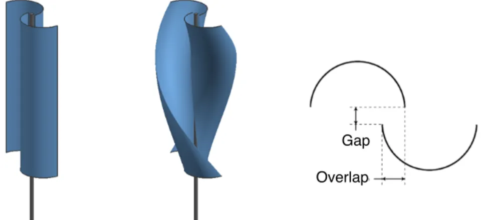
(19) This investigations focuses on the Savonius WT. This kind of device was invented by a Finnish engineer called Sigurd J. Savonius in 1922 and it was patented in 1926. It is classified as a vertical axis wind turbine (VAWT) although it can be installed horizontally or diagonally also. Aerodynamically its principle is based on the difference of the drag force that the wind exerts over the two blades whose profile its similar to an “S” (See Figure 2). The force difference is generated because when the air gets in contact with the blades one of those is concave and the other is convex according to the wind direction. This cause an effect that will try to move both blades in different directions but because the force exerted over the concave blade is superior that the force exerted over the convex blade the rotor will rotate.. Wind. Figure 2. Typical profile of a Savonius WT rotor.. The change of the rotor shape according to the wind direction when the rotor is in movement will cause a cyclic load. In order to avoid that kind of behavior it was developed the helical Savonius. With the helical shape it is assure that a constant load will be applied to the electric generator, the vibration will be eliminated and the WT will be able to start with any wind direction. The helical Savonius presents advantages over the HAWT that makes them capable to be installed on urban media. Some of the advantages are the following:. -. It doesn’t generate noise because the velocity of rotation doesn’t exceed the wind velocity.. -. It doesn’t generate vibrations because of its helical shape and this allows them to be installed on buildings.. -. It is safe with the animal life because its blades seems like solid objects. It doesn’t need to be oriented to the wind (omni-directional) It can generate electricity with turbulent winds due to its omni-directional capacity. Starts at 1 to 3 m/s (10.8 km/hr, 7.75 MPH).. 5.

(20) -. Low maintenance as consequence of its low working speed and its few mobile parts. It can be manufactured with low cost materials and processes It can be installed in any position (but only the vertical is omni-directional). Attractive design. It can be installed on places with low average speeds as 4.5m/s (excellent for urban media).. On the other hand, the disadvantages are:. -. Less efficient than the HAWT. The helical model has a complicated geometry. The general idea is that this is an obsolete technology. The actual market offers this kind of device at very high prices.. This characteristics point to the opportunity areas of this technology, and here is where it can be researched to offer a superior product for the society. From those points, the low efficiency according to the HAWT will be the focus on the present investigation. 2.1.2. Efficiency The efficiency or CP of a WT is defined as the total power extracted by the device over the total power of the wind, as expressed on the equation 5.. 5 As the power of the wind can be expressed with the equation 4 and the power of a rotating body is equal to the torque times its angular velocity, the equation 6 can be expressed as follows.. 6 As the optimization of the CP is the main objective of this investigation, in this section it is shown the main improvements made to the Savonius WT according to this characteristic since the beginning of this technology. On the Figure 3 it is shown the CP of the most common types of WT’s in which this parameter variates according to the TSR. This is because each wind turbine has an optimum working velocity, this velocity is called tip speed ratio (TSR or !) and it is the relative. 6.

(21) velocity of the tip of the blade according to the wind velocity regarding to the equation 7. For the Savonius WT the TSR is around 0.8 to 1.. 7. Figure 3. CP according to the TSR for the most common WT’s. [Becker, 2006]. On the last Figure it is clear that the Savonius rises at a maximum CP over 30% compared with the 45% of the HAWT’s. In the same Figure, a theoretical limit called the Betz’ law is shown. This limit was determined in 1919, and it affirms that the device can extract a maximum of 59.26% of the wind energy.. 8 It must be clear that the limit shown in Figure 3 shows the Betz limit for propeller type WT, so this diminishing of the CPmax at lower TSR is only for HAWT’s. The Betz law supports the fact that the WT needs to take energy from the wind, this involves taking out velocity from it. So if you take velocity from it, the mass flow rate over the WT rotor will decrease and this will impact negatively in the power output. So there is a tradeoff between the velocity taken out from the air and the mass that passes through the rotor. This tradeoff is satisfied at its optimum point when the wind velocity at the outlet is 1/3 times the velocity of the inlet and these reaches the CPmax shown on Equation 8.. 7.

(22) As an example, the power of a 10m/s wind that passes through an area of 1m2 has approximately a power of 612.5 watts. From this total power of the wind, if the most efficient WT is built, it will be able of extracting only 363 watts according to the Betz law. 2.1.3. Evolution of the Savonius wind turbine It is known that in order to maximize the CP it is needed to modify the shape of the rotor because it is the responsible of capturing the kinetic energy of the wind and convert it into mechanical energy. For that reason the profile of the rotor is the principal point of interest, while the diameter may be a factor that can improve the performance. In order to improve the efficiency of the Savonius WT there have been different investigations. All of this investigations have focused in shapes using profiles with a constant thickness in order to make them easy to manufacture. In the Table 1 are shown the principal improvements made to the CP modifying the rotor profile. Table 1. Savonius rotor CP improvements.* Rotor. Patent date. Savonius. Benesh. *. TSR. CP. Reference. 0.85. ~26.5. Blackwell 1977*. 0.85-1.15. ~27. Moutsoglou 1995*. NA. 33. US Pat. 4,784,568. 0.85-1.15. ~29.5. Moutsoglou 1995*. Profile Shape. 1926. 1988. Benesh. 1996. NA. 37. US Pat. 5,494,407. Rahai. 2008. 1.45. >40. US Pat. 7,393,177. Wind tunnel test. 8.

(23) 2.1.3.1. Savonius rotor The typical Savonius rotor consists in two semicircular buckets and has been improved on a couple of investigations. These projects claim that they have obtained shapes with superior CP’s. The first formal research in this field was made by Blackwell in 1977. The improvement consisted in the creation of several one meter diameter wind turbines with two and three buckets and different overlaps. This investigation carried out by the prestigious SANDIA laboratories concluded that the optimum ratio overlap/diameter was between 0.1 and 0.15 reaching a CP of approximately 26.5%. One research was made by Valdès and Ramamonjisoa (2006) in which the optimal shape was obtained using an algorithm that modified the shape of the device. This shape modification was limited to semicircular blades in order to manufacture them with oil drums. On this investigation the design variants for improving the CP were evaluated with a mathematical model that described the behavior of this WT. Another research was made by Menet and Bourabaa (2003). They made variations to the overlap/diameter ratio in order to increase the CP. The CP on that investigation was obtained through a CFD analysis which is not detailed in the publication. The range of values evaluated for the ratio was 0.1 to 0.5 and they concluded that the optimum performance was obtained at a ratio overlap/diameter of 0.242.. Gap Overlap. Figure 4. a) Savonius wind turbine b)Helical Savonius wind turbine, c) Savonius rotor profile.. 9.

(24) 2.1.3.2. Benesh rotor Alvin H. Benesh developed two rotors with superior performance than the existing technologies at those times. The first was developed in july of 1987 and the patent 4,784,568 was released on november of 1988. In the patent, Benesh claims that its rotor reaches a CP of 33%.. Figure 5. Benesh rotor shape. [Benesh, 1988]. The second design was developed in december of 1994 and in february of 1996, the patent 5,494,407 was released. In that document, the rotor shown in the Figure 6 was presented and according to Benesh, it could achieve a CP of 37%.. Figure 6. Benesh rotor shape. [Benesh, 1996]. 2.1.3.3. Rahai rotor This model is the newest development in the modification of a Savonius rotor. It was developed by Hamid R. Rahai in november of 2005 and the patent 7,393,177 was released on july of 2008. The rotor shape is presented in the Figure 7.. 10.

(25) Figure 7. Rahai rotor shape. [Rahai, 2008]. This investigation consisted in an optimization of the Benesh (1988 Patent) profile, modifying it through the use of Hicks-Henne functions. The strategy of shape modification produced shapes as the ones shown in the Figure 8. It should be noted that Rahai also added one factor to the shape modification that is not shown in that Figure; that is the overlap. Those shapes were then evaluated using a computational fluid dynamics (CFD) 2D steady analysis.. Figure 8. Shape variations made by Rahai. [Rahai, 2008]. The optimization process was carried out implementing a non-linear sequential quadratic programming scheme using a multidisciplinary design optimization (MDO) software. In this case the MDO software used was iSIGHT. This process was completely automated and the result is compared with the initial design in the following Figure.. Figure 9. Initial (Benesh 1988) and optimized profile. [Rahai, 2008]. 11.

(26) The results are changed when the overlap ratio is reduced to zero. The maximum power coefficient for the optimized blade is more than 0.4 for the mean velocities of 6.8 and 9.75 m/sec and about 0.4 In for the mean10, velocity of 8.0 m/sec. These thanwith 30% improvements figure Rahai compares thevalues CP ofareitsmore rotor Benesh’s 1988 CP and the CP of the over the power coefficient of the Benesh airfoil. The rise in the power coefficients extends to a tip speed ratioSavonius of 1.6, before it starts decrease.mention These results consistent with at ourwhich numerical rotor. It todoesn’t the are wind velocity it was evaluated but it does analysis and indicate that the optimized blade can sustain power generation up to a much higher the values for the Benesh and Savonius rotor where obtained by Moutsoglou and tip speed ratiosay than that the Benesh or Savonius airfoils.. Weng. (a). (b) Savonius Benesh 6.80 m/sec 8.00 m/sec 9.75 m/sec. 0.5. Savonius Benesh 6.80 m/sec 8.00 m/sec 9.75 m/sec. 0.4. Power Coefficient, Cp. Power Coefficient, Cp. 0.4. 0.3. 0.3. 0.2. 0.2. 0.1. 0.1 0.0 0.0. 0.2. 0.4. 0.6. 0.8. 1.0. 1.2. 1.4. 1.6. 1.8. 0.2. 2.0. 0.4. 0.6. 0.8. 1.0. 1.2. 1.4. 1.6. 1.8. 2.0. 2.2. Tip Speed Ratio, !. Tip Speed Ratio, !. Figure 10. CP comparison for the Rahai, Benesh 1998 and Savonius rotors. [Rahai, 2008]. Figure 15. Variation of power coefficient at different velocities for blades without the slot at (a) 48% blade overlap and (b) zero blade overlap.. The optimized rotor has the shape specified on Figure 7. It is worth mentioning that it is (a). (b). only the blade’s shape and it must be added the overlap. In this case the zero overlap design Savonius was the one with better performance. Benesh. 0.5. 6.80 m/sec 8.00 m/sec 9.75 m/sec. Power Coefficient, Cp. 0.4. On Figure 11 it is shown one of the 2D steady CFD analysis. It is a velocity contour of the optimized blade with an overlap of 48%.. 0.3. 0.2. 0.1. 0.0 0.2. 0.4. 0.6. 0.8. 1.0. 1.2. 1.4. 1.6. 1.8. 2.0. 2.2. Tip Speed Ratio, !. Figure 16. Variation of power coefficient at different velocities for blades with the spanwise slots at (a) 48% blade overlap and (b) zero blade overlap.. When the spanwise slots are in place, for the 48% overlap condition, the increase in the power coefficient of the optimized blades is not as significant as before. The maximum power. Figure 11. 2D Steady CFD analysis of a Rahai rotor with 48% of overlap ratio. [Rahai, 2005] 23. With this results it can be concluded that the optimized rotor can generate electricity Figure 14. Velocity Contours for the two-blade system at 15 degrees angle of attack. rotating at higher angular speed than the rest of the Savonius rotors. The patent declares that rotor cannumerical achieve studies a CP superior to 40% at a TSRsingle of 1.5. Thisshould results must be taken The this results of the indicate that the optimized blade produce higher torque than the baseline blade. However, the presence of the spanwise slot results in with discretion given that they don’t present neither wind tunnel tests nor any of their CFD larger flow separation regions and loss of momentum which should result in reduced torque and analysis parameters. Furthermore the CFD analysis was performed steady and due to the lower performances.. nature of the Savonius rotor, it must be evaluated as unsteady.. For the optimized two-blade configuration with the large overlap the flow does not completely encompass the whole blades as it did for the single blade and thus should not have significant improvements in the overall drag force. For the two-blade configuration, improvement is expected when the overlap percentage is significantly reduced. For experimental study, the focus was on the performances of the optimized two-blade configuration with and without the spanwise slots at zero and 48% overlap conditions.. 12.

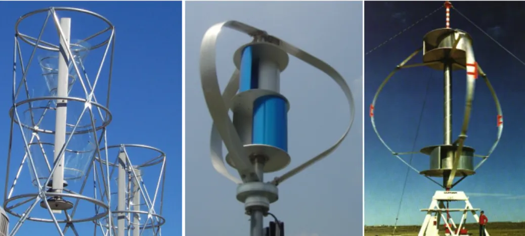
(27) 2.1.3.4. Hybrid wind turbines Another Savonius wind turbine has been developed using a combination of two different VAWT’s. This development has two different origins. The first development was made some decades ago, in order to assist the Darrieus WT on the starting given it could not start by itself. The second development appeared as an intent to improve the CP of the Savonius WT. It was invented by William S. Becker and the patent was released on november of 2006. He declared that his hybrid VAWT could reach a CP higher that 30% at TSR around 2 (See Figure 3). This means that the working velocity is higher than any of the previous Savonius rotors.. Figure 12. Combination of Savonius-Darrieus rotors, Becker at left and traditional combination at center and right. [generated by the author according to different internet sources]. 2.1.4. Market overview The necessity to electrify zones that don’t have access to the electric grid have impulsed the presence of different kinds of devices that take advantage of alternative sources of energy such as low scale wind and solar energy systems between 50 and 2000 watts. This needs have created a new niche market that has been filled with products especially designed to meet the necessities of this kind of lone places. Those devices include wind turbines, photovoltaic cells and solar boilers and are now considered as mature products. On the other hand, the development of that kind of devices, the rising of the fossil fuel prices, and the growing interest of the people to reduce their impact in the environment has created a new market opportunity that include urbanization's with access to the electric grid. This new consumers can be connected to both their renewable energy devices and to the electric grid to consume electricity from it when the devices aren’t taking energy from the wind or/and sun. This kind of grid/device connection can reduce a big percentage of the. 13.

(28) monthly electricity bill and at the same time it reduces the negative impact to the environment. This new market has created new companies that offer a wide variety of small HAWT but on the last years, there are arising some VAWT that have better characteristics to make them suitable for the urban media. According to the American Wind Energy Association (AWEA), the U.S. small wind turbine market grew 14% and deployed 9.7 MW of new capacity on 2007. This small WT market consists of devices with a capacity bellow 100 kW and an average of approximately 1 kW. On the Figure 13 it is clear that in the year 2005 the sales went down in an alarming rate. That is explained because in California -the principal consumer of this kind of technologythe incentives for small wind systems decreased dramatically in 2004.. Figure 13. Growth of U.S. small wind market. [AWEA, 2008]. The application of incentives on this kind of technology increases the demand for this products. According to AWEA, “In its current (and historic) state without a federal-level incentive to assist consumers purchase small wind systems, the U.S. market continues to grow an estimated 14-25% annually. Grid-connected, residential-scale systems 1-10kW in capacity constitute the fastest growing market segment.[...] The advent of a 30% federal Investment Tax Credit could lead to an estimated 40-50% annual growth, similar to that experienced by the U.S. solar photovoltaic (PV) industry with the. 14.

(29) 2005 creation of such a credit. AWEA, its allies, and industry are actively advocating for legislation that would create a 30% credit for turbines 100kW and under.” (AWEA; 2008: 3) On Figure 14 the increase on the sales of on-grid WT’s with capacities greater than 1kW is visible and it gives us very important information of the tendency of the market.. Figure 14. U.S. market: On-grid Vs. Off-grid. [AWEA, 2008]. 2.2. Computer aided design The computer aided design (CAD), is a software that is primarily used on the engineering, design and architecture industry. The main function of this tool is to aid the design and elaboration of technical drawings of products. This software is capable of modeling 2D and 3D drawings, surfaces and solids that virtually represents products or parts of them. The 2D model creation is commonly driven by basic shapes as lines and arcs that are placed together in a plane. On the other hand to create 3D solids, different kind of features like extrusions, revolves or sweeps are applied to the mentioned basic shapes. Then those solids are detailed with features like rounds, chamfers, boolean operations, among others. The next Figure exemplifies a 2D and a 3D model.. 15.

(30) 2005 creation of such a credit. AWEA, its allies, and industry are actively advocating for legislation that would create a 30% credit for turbines 100kW and under.” (AWEA; 2008: 3) On Figure 14 the increase on the sales of on-grid WT’s with capacities greater than 1kW is visible and it gives us very important information of the tendency of the market.. Figure 14. U.S. market: On-grid Vs. Off-grid. [AWEA, 2008]. 2.2. Computer aided design The computer aided design (CAD), is a software that is primarily used on the engineering, design and architecture industry. The main function of this tool is to aid the design and elaboration of technical drawings of products. This software is capable of modeling 2D and 3D drawings, surfaces and solids that virtually represents products or parts of them. The 2D model creation is commonly driven by basic shapes as lines and arcs that are placed together in a plane. On the other hand to create 3D solids, different kind of features like extrusions, revolves or sweeps are applied to the mentioned basic shapes. Then those solids are detailed with features like rounds, chamfers, boolean operations, among others. The next Figure exemplifies a 2D and a 3D model.. 15.

(31) Figure 15. 2D and 3D part modeled on a CAD software.. The dimensions and positions of the lines and arcs mentioned on the last paragraph can be defined by parameters with values that can be changed. This changes of values generates modifications to the model and can be defined in order to facilitate the model modification. This kind of technique is called parametric modeling. It can be useful to modify models but the possibilities are limited by the parameters defined at the moment of the creation of the model. On Figure 16 it is illustrated a parametric model with different parameter values. In it the height, radius and thickness of the handle where modified.. Figure 16. Modifications to a parametrized model.. Another kind of shape that can substitute the lines and arcs is commonly called spline. This shape is a curve defined piecewise by polynomials and its correct name is B-spline which is a generalization of the Bézier curve. It is created by adding control points that define the position of the curve. From this points only the first and the last are in contact with the curve, the other points only serve as “magnets” that attracts the curve in a smooth way as seen on Figure 17. The smoothness of the curve can be modified by changing the degree of the B-spline. This degree can be set as linear, quadratic, cubic, or greater, but it needs to have a degree smaller than the number of control points on the curve. There is another approach called interpolation B-spline. This technique differs from the simple B-spline because with this approach all the control points are in contact with the Bspline curve. This difference can be observed on Figure 17 and makes it superior in the CAD parametric modeling.. 16.

(32) Figure 17. Quadratic b-spline (left) and quadratic interpolation b-spline (right).. The parametric modeling using B-splines can offer superior possibilities when trying to modify a model. On Figure 18 is shown a model made with B-splines that has been modified. Such modifications can produce shapes that a combination of circles and lines never could generate.. Figure 18. Modifications to a parametrized model created with splines. [Cueva, 2006]. 2.3. Computer aided engineering This technology is another of the computer aided field (CAx). It is a tool that helps the engineering teams to simulate, analyze, and manufacture products virtually. This can save money and time to the development of new products because it decrease errors and helps to design robust products and processes. The CAE includes areas like Finite Element Analysis (FEA), Computational Fluid Dynamics (CFD) and Multibody Systems.. 17.

(33) Figure 17. Quadratic b-spline (left) and quadratic interpolation b-spline (right).. The parametric modeling using B-splines can offer superior possibilities when trying to modify a model. On Figure 18 is shown a model made with B-splines that has been modified. Such modifications can produce shapes that a combination of circles and lines never could generate.. Figure 18. Modifications to a parametrized model created with splines. [Cueva, 2006]. 2.3. Computer aided engineering This technology is another of the computer aided field (CAx). It is a tool that helps the engineering teams to simulate, analyze, and manufacture products virtually. This can save money and time to the development of new products because it decrease errors and helps to design robust products and processes. The CAE includes areas like Finite Element Analysis (FEA), Computational Fluid Dynamics (CFD) and Multibody Systems.. 17.

(34) To use a CAE software it is needed to follow three steps, the first is the pre-processing, the second is the analysis solver and the third is the post-processing. On the pre-processing stage the virtual model is defined and discretized dividing it in small sections or elements. The group of elements is defined as a mesh. Then the initial and boundary conditions are set. This conditions are the forces applied to the model, material properties, movement of parts, among others. Finally the solver is defined. This involves the selection of equations of motion, turbulence, species, among others. The second stage involves the analysis of the model defined on the first stage. This stage can be highly demanding with the workstation. Some analysis are restricted to very powerful computers. On the third stage the results are analyzed using visualization and plotting tools. This tools can show the loads, power, energy, temperature or whatever the engineer is analyzing. 2.3.1. Mesh As the previous section mentioned, the mesh is the discretization of the model that is being analyzed. That force us to create a detailed mesh to obtain an accurate representation of the model in order to obtain good results. Depending on the model, every mesh is composed by several 2D and/or 3D elements. Every element is defined by nodes positioned on each vertex and the second order elements have one more node positioned on the center of every edge. On the Figure 19 are illustrated the most common types of elements. The first column illustrates 2D elements, the first two are called triangular (tri) and quadrangular (quad), the next two are are defined as second order tri and second order quad. The second column shows tetrahedral (tet), pyramid, pentahedral (also called wedges and triangular prisms) and hexahedral (hex) elements. On the third column can be observed the same as in the second column but defined as second order. It can be notice that the second order elements has more nodes, this generates more precise results but also it demands a more powerful computer to solve it.. 18.

(35) element configuration tells HyperMesh how to draw, store, and work with the element. The element type allows you to define multiple analysis elements for each HyperMesh element.. Element Configuration The element configuration defines the physical geometry (i.e., quad, hex) of the element. Element configurations include:. Figure 19. Most common element types. [Altair Engineering, 2007] Altair Engineering. HyperMesh 8.0 User’s Guide 27 Proprietary Information of Altair Engineering. To create a mesh first it is needed to define the size, number or density of elements desired on each edge. Then the surfaces are meshed with tri, quad or mixed elements according to the mesh of the edges. The next step (only for 3D models) is to mesh the solids using any kind of elements, this mesh is created according to the surfaces mesh. On the Figure 20 can be seen a representation of a 2D tri mesh and a 3D hex mesh.. Figure 20. Examples of a 2D and 3D mesh. [Fluent, 2006]. The mesh creation is made automatically by the software according to the defined mesh size. This automatic process is very simple when using tri/tet elements but in the case of the quad/hex it can be very time consuming and require some experience. The reason of continuing using this kind of elements is its superior accuracy over the rest kind of elements. According to Fluent,. 19.

(36) “For simple geometries quad/hex meshes can provide high quality solutions with fewer cells than a comparable tri/tet mesh. [...] For complex geometries, quad/hex meshes show no numerical advantage, and you can save meshing effort by using a tri/tet mesh.” (Fluent; 2001: 2-9) There are two kinds of mesh according to the elements distribution on the model, the unstructured or paved and the structured or mapped (Shown in Figure 21).. Figure 21. Comparison of unstructured (left) and structured (right) meshes. [ANSYS, 2007]. The unstructured mesh is the most easy to create. It is made defining only the density or size of the elements on every face of the model and is generated automatically with any kind of elements. On the other hand the structured mesh is a more accurate way of discretizing the models but it is considerably more difficult to create. It can be created with any kind of elements but mainly it is used with quad and hex. Due to the difficulty of meshing this kind of elements the meshing process commonly fails and require some changes in the mesh size or a different meshing approach. On CFD analysis is common to find another characteristic in the elements. It is a more detailed mesh that is placed on the edges that has a interaction between solids and fluids. It is called boundary layer and it is created to generate more accurate results in the zones with fluid/solid interaction where the laminar/turbulent transition flows should appear.. Figure 22. Boundary layer. [Fluent, 2006]. 20.

(37) 2.3.2. Computational fluid dynamics This tool is used to model and measure the flow of fluids. To this flow it can be added heat, mass transfer, phase changes, chemical reactions and interaction with moving solids in order to accurately represent the analyzed system or device. The CFD codes are based on two main aspects, the physical modeling and the numerical methods. The physical model translate the information of the analyzed system or device contained on the mesh into a set of equations that relate the governing equations of mass, momentum (Navier-Stokes equations) and energy conservation (thermodynamics 1st law). There are different approaches to compute this task. The most used methods are finite volume method (FVM), finite difference method and finite element method. From this approaches the FVM is the most widely used in commercial CFD software such as: Fluent, STAR-CD, CFX, OpenFOAM, Phoenics, FloWorks, Numeca, among others. When this task finishes it process ti creates a set of partial differential equations that needs to be solved. The numerical method is in charge of solving that differential equations. To complete that task the numerical method first needs to transform each differential term into an algebraic relation. This transformation can be done with different techniques for every set of equations. The momentum or Navier-Stokes equations are typically solved using SIMPLE, SIMPLER, SIMPLEC or PISO methods. For other terms such as turbulence, convection, etcetera, there are methods such as first order upwind, second order upwind and QUICK. The transformation of the differential equations creates a linear system of equations that can be solved using iterative methods. Typical direct methods cannot be used because they are computationally expensive, inefficient for large sparse matrices and the non-linearity of the coefficient of the system’s matrix forces to use iterative methods. This iterative method compute the results of the CFD analysis until it converges, another way saying it, is that it will compare the results of the new computation with the results of the las computation and when the error stays lower than the user defined value, the solution is reached. When the analysis is time dependent it must be added one more consideration, the time. The CFD analysis can be steady when the flow reaches a point where the solution converges or unsteady when the fluid never reaches a steadiness and it can be caused by the creation of vortexes or because the physical model involves solids in movement or cyclic. 21.

(38) flows. For the unsteady analysis the term of time should be added to the conservation equations. This forces us to discretize it and it can be done as first or second order. The unsteady analysis consist in an analysis that will be computed several times. The separation in time of every one of those analysis is defined as time step size (TSS) and it will consist in as many time steps (TS) as needed, usually until a cyclic result that doesn’t change is observed. The pre-processing stage of a common CFD analysis consists in the following steps:. -. Import the mesh file. Solver selection: this step consist in the selection of the type of analysis, discretization. -. method for the time and conservation equations, turbulence models. Operating conditions: Conditions such as gravity, operating temperature and operating. -. pressure. Boundary conditions: The conditions of the physical model are set in this step. Pressure inlet, velocity inlet, pressure outlet, velocity outlet, outflow, mass flow inlet, fan, wall, symmetry, porous media and radiator are some of the possible boundary conditions.. -. Initial conditions: This conditions are a initial guess of the results that the analysis is going to generate. Usually it is defined as a velocity, pressure and turbulence intensity that is assigned to the surfaces and solids, but there is another approach defined as interpolation. This approach consist in taking the results from another similar solved. -. analysis that can be a more close initial guess and can save computation time. Residuals: Here the user select the accuracy of the results by defining the acceptable. -. value for the residuals. Solve: In this step the the number of iterations is defined for steady analysis and the TSS, TS and number of iterations for each time steps is defined for unsteady analysis.. After the convergence is reached. The user can obtain the results as an image with contours, vectors or as a plot. Some of possible results that can be computed are pressure, total pressure, dynamic pressure, density, velocity magnitude, density, temperature, turbulence intensity, among others. On the Figures 23 and 24 it is observed the resultant total pressure contour and velocity vectors for the analysis of a 2D blower.. 22.

(39) Figure 23. CFD total pressure contour. [Fluent, 2006]. Figure 24. CFD velocity vectors. [Fluent, 2006]. Some other considerations must be defined when a CFD analysis is performed. One of them is the compressibility of the fluid that can be neglected when the Mach number (M) in the system is much less than 1 (M<0.1). Another consideration is the type of flow that is going to be analyzed, it can be inviscid, laminar of turbulent. The turbulence is a fluid flow that seems to be random and chaotic in 3 dimensions and it is very difficult to accurately modeling it. There are different models to describe this kind of phenomena such as Spalart-Allmaras, k-$ Standard, k-$ RNG, k-$ Realizable, k-# Standard, k-# SST, Reynolds stress, detached eddy simulation and large eddy simulation. From these models only the Splarat-Allmaras, k-$, k-# and Reynolds stress method can be applied in 2D simulations in the most common commercial CFD codes. From these models the k-$ is the simplest of the “complete models” and according to Fluent, “The standard k-% model in FLUENT falls within this class of turbulence model and has become the workhorse of practical engineering flow calculations in the time since it was proposed by Launder and Spalding. Robustness, economy, and. 23.

(40) reasonable accuracy for a wide range of turbulent flows explain its popularity in industrial flow and heat transfer simulations.” (Fluent; 2006: 12-12) The standard k-$ model has been modified to improve its performance in different flow conditions. From those developments, the Realizable k-$ model “provide superior performance for flows involving rotation, boundary layers under strong adverse pressure gradients, separation, and recirculation” mentioned Fluent (2006).. 2.4. Genetic algorithms A genetic algorithm (GA) is a searching technique based on the evolution of species and genetics. From the evolution of the species, the GA’s has taken the techniques of selection according to fitness, crossover (also called recombination or hybridization) and mutation. From the genetics field, the GA’s use the codification of the chromosome (also called genotype) as basis to code in strings the search space of a problem. Therefore the search can be performed modifying the chromosomes until the objective is reached. As mentioned, the genotype is expressed as a string of genes that are represented with numbers (0001011101) in any numeral basis although the most common is the binary representation. This genotype can be translated to some characteristics called phenotype. An analogy to this can be that some person has certain gene o group of genes into its chromosome that represents green eyes, this representation of the genotype is defined as the phenotype. On Table 2 it is presented a representation of the genotype, phenotype and fitness. In this Table is shown a binary genotype on the first column that is translated to its phenotype form which in this case is the value for the variable x. This translation is made by converting the binary number value to decimal. Then the fitness is calculated with a specified function, simulation or analysis, which in this case is the equation 9. 9. 24.

(41) reasonable accuracy for a wide range of turbulent flows explain its popularity in industrial flow and heat transfer simulations.” (Fluent; 2006: 12-12) The standard k-$ model has been modified to improve its performance in different flow conditions. From those developments, the Realizable k-$ model “provide superior performance for flows involving rotation, boundary layers under strong adverse pressure gradients, separation, and recirculation” mentioned Fluent (2006).. 2.4. Genetic algorithms A genetic algorithm (GA) is a searching technique based on the evolution of species and genetics. From the evolution of the species, the GA’s has taken the techniques of selection according to fitness, crossover (also called recombination or hybridization) and mutation. From the genetics field, the GA’s use the codification of the chromosome (also called genotype) as basis to code in strings the search space of a problem. Therefore the search can be performed modifying the chromosomes until the objective is reached. As mentioned, the genotype is expressed as a string of genes that are represented with numbers (0001011101) in any numeral basis although the most common is the binary representation. This genotype can be translated to some characteristics called phenotype. An analogy to this can be that some person has certain gene o group of genes into its chromosome that represents green eyes, this representation of the genotype is defined as the phenotype. On Table 2 it is presented a representation of the genotype, phenotype and fitness. In this Table is shown a binary genotype on the first column that is translated to its phenotype form which in this case is the value for the variable x. This translation is made by converting the binary number value to decimal. Then the fitness is calculated with a specified function, simulation or analysis, which in this case is the equation 9. 9. 24.

(42) Table 2. Representation of genotype, phenotype and fitness.. Genotype or Chromosome. Phenotype or Variable value. Fitness or Evaluation. 10101. 21. 96.23. 00110. 6. 14.69. 10001. 17. 70.09. The genotypes can represent more than one variable. The example shown in the Figure 25 represents a 10 bits genotype formed by two variables, each one with a length of 5 genes. Each of this group represents a variable that can be decoded changing it numeral basis from binary to decimal. In this example the variable x ( 0 1 0 1 0 ) represents a decimal value of 10, and the variable y ( 1 1 0 0 1 ) represents a value of 25. As the length of both sets of genes are 5, each of this variables can represent 31 (25-1) possible of combinations. x. y. 0101011001 Figure 25. Genotype representation with two variables.. Supposing that a GA is trying to obtain the values for x and y that maximize the equation 10 using the genotype defined on the last Figure. It can be concluded that the variable x will have 31 possible values to search for an optimum between 0 and 2 and the variable y will have the same 31 possible values between 0 and 1.. 10 So for the variable x the genotype 00000 will represent the value 0 and the genotype 11111 will represent the value 2. The values between this limits will be obtained when changing the value of the genotype in it binary basis and it will represent 31 values between them. The process of a GA can be explained with the next steps, and it can be observed on the Figure 26. 1. Genotypical representation selection: The first step to implement a GA is to select the type of codification of the genotype. In order to complete this task, it is needed to define the numeral basis, number of variables and length of genes for every variable. The length. 25.

(43) of every coded variable needs to be defined with enough resolution in order to achieve the optimization task. 2. Initial population generation: It must be defined the number of individuals for the initial population and its values. By default this is defined randomly, but they can be defined manually. 3. Individual evaluation: Once the population is ready, the evaluation takes place. Depending on the problem, the evaluation can be an equation, simulation on CAE software or any situation that offers an evaluation of the fitness. 4. Reproduction: This task divides in three stages that are inspirited in the evolution of species. It is a very important step because in it takes place the creation of new individuals. a. Selection: In this stage the individuals with better fitness according to the objective are selected to breed a new generation of individuals. b. Crossover: Here the selected individuals on the last stage are placed in pairs and then their genotypes are crossed using a crossover operator. This operator cuts each genotype in a random gene and then changes the sections after the cut from one individual to the other. This process generates two child's from two parents. The occurrence of this process can be present in every set of parents but also it can be defined to occur with a defined probability. c. Mutation: This operator consist in randomly change the value of the bits inside a genotype. It is used with a low probability of occurrence in order to generate “errors” in some individuals. This has the propose to avoid local optima by preventing similar genotypes becoming to similar to each other. 5. The steps 3 and 4 repeats until the GA reaches the objective.. 26.

(44) Selection of genotype representation Initial population generation Evaluation of phenotypes. Selection Crossover Mutation. Solution. Reproduction. Termination criteria. New generation. Figure 26. Diagram of a genetic algorithm. [Arcos, 2006]. 27.

(45) Chapter 3. Methodology On this chapter, the methodology used for the optimization of the Savonius rotor is presented. It consists in the automation of the optimization process aided by multidisciplinary design optimization (MDO) software. The optimization consists in the improvement of the wind turbine performance modifying the shape of the rotor profile and the TSR. Inside the MDO environment are different types of optimization algorithms that can be chosen. Among these, a genetic algorithm was selected to direct the automated design optimization process. In this automated process, different kinds of softwares were involved to carrie out different tasks. First, a CAD software is needed to modify the shape of the Savonius rotor, then a meshing software discretize the geometry created with the CAD system. After that, a 2D CFD analysis is carried out to calculate the CP of the shape. At the end of this process, the GA inside the MDO software analyzes the results of the generation of individuals and generates the child’s that will be analyzed on the next generation.. 3.1. Strategies for the integration of the optimization process The mentioned process is simple, but it needs the knowledge of CAD, CAE such as mesh software and CFD and MDO software. Also it requires the ability of integrating all of this softwares using automating strategies such as macros, journals and DOS script. In this section the strategies used for the setup of the automated process are presented. First, the modification of the model in CAD is described. Then, the mesh technique used is analyzed. This is followed by the CFD analysis and the process of reading the results.. 28.

(46) Chapter 3. Methodology On this chapter, the methodology used for the optimization of the Savonius rotor is presented. It consists in the automation of the optimization process aided by multidisciplinary design optimization (MDO) software. The optimization consists in the improvement of the wind turbine performance modifying the shape of the rotor profile and the TSR. Inside the MDO environment are different types of optimization algorithms that can be chosen. Among these, a genetic algorithm was selected to direct the automated design optimization process. In this automated process, different kinds of softwares were involved to carrie out different tasks. First, a CAD software is needed to modify the shape of the Savonius rotor, then a meshing software discretize the geometry created with the CAD system. After that, a 2D CFD analysis is carried out to calculate the CP of the shape. At the end of this process, the GA inside the MDO software analyzes the results of the generation of individuals and generates the child’s that will be analyzed on the next generation.. 3.1. Strategies for the integration of the optimization process The mentioned process is simple, but it needs the knowledge of CAD, CAE such as mesh software and CFD and MDO software. Also it requires the ability of integrating all of this softwares using automating strategies such as macros, journals and DOS script. In this section the strategies used for the setup of the automated process are presented. First, the modification of the model in CAD is described. Then, the mesh technique used is analyzed. This is followed by the CFD analysis and the process of reading the results.. 28.

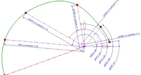
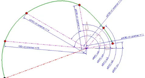
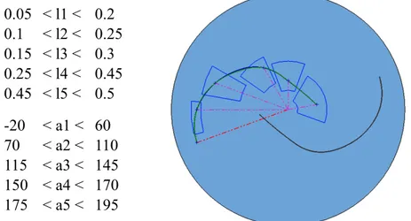
(47) Finally the GA used is described and the integration of the whole process in the MDO software is discussed. All of this tasks automated by macros and journals must be able of analyzing different rotors shapes and at different TSR. For that reason, the variables of the design shape and the operation conditions such as the TSR must be introduced to the macros and journals of every design iteration. In order to do that, the MDO software is capable of editing the macros and journals adding this variables in the correct position of the text. 3.1.1. CAD For the modification of shape propose, first a parametric 2D model of the Savonius rotor was created using the commercial software Unigraphics NX5. As it needed to have enough flexibility to generate a big space of search it was decided to create it using interpolation Bsplines. This curve was created using six control points that could be moved changing its position using a polar coordinate system as seen on Figure 27. From this control points only the black one was fixed, the other five points was defined as variables. The angles were named from a1 to a5 and the lengths were defined from l1 to l5. The lengths were defined as a proportion of the diameter, so in case of a diameter length change their values also change to form the same shape. This strategy is useful if the GA used the diameter as a variable to optimize because using certain values of l1...l5 with different diameter values the shape will have the same appearance but with different size.. Figure 27. Parametrized interpolation B-spline used to model one blade of the rotor.. 29.

(48) Finally the GA used is described and the integration of the whole process in the MDO software is discussed. All of this tasks automated by macros and journals must be able of analyzing different rotors shapes and at different TSR. For that reason, the variables of the design shape and the operation conditions such as the TSR must be introduced to the macros and journals of every design iteration. In order to do that, the MDO software is capable of editing the macros and journals adding this variables in the correct position of the text. 3.1.1. CAD For the modification of shape propose, first a parametric 2D model of the Savonius rotor was created using the commercial software Unigraphics NX5. As it needed to have enough flexibility to generate a big space of search it was decided to create it using interpolation Bsplines. This curve was created using six control points that could be moved changing its position using a polar coordinate system as seen on Figure 27. From this control points only the black one was fixed, the other five points was defined as variables. The angles were named from a1 to a5 and the lengths were defined from l1 to l5. The lengths were defined as a proportion of the diameter, so in case of a diameter length change their values also change to form the same shape. This strategy is useful if the GA used the diameter as a variable to optimize because using certain values of l1...l5 with different diameter values the shape will have the same appearance but with different size.. Figure 27. Parametrized interpolation B-spline used to model one blade of the rotor.. 29.

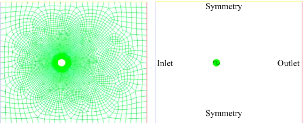
(49) The next step in the model generation is to apply a thickness to the curve created before and round it on the extremes using a radius equal to the half of the thickness so that the shape had tangent edges. This thickness can also be used as a variable in the optimization process. The next step was to generate a rotated copy and positioned it at 180 degrees to create the second blade of the rotor. After the rotor was defined, the next step was to determine the fluid zone that was going to be analyzed with CFD. This zone needed to be divided in two surfaces. The first is the rotor zone: it needed to have a circular shape with the rotor centered in it, also it needed to have a space between the tip of the blades and the edge of the surface. A 10% of the rotor diameter was used as the separation mentioned before. The second zone was the fluid around the rotor. This zone was needed in order to avoid tunnel effects that concentrate the fluid, which are negative in the analysis and must be avoided. Cochran et al in 2004 used a fluid zone with a size of 10 turbine diameters for each direction. For this zone, ti was increased the size in the direction to the outlet (right) in order to minimize the influence of the boundary condition of the outlet (Pressure=0). On the next Figure it can be observed the two zones and three rotor modifications of the traditional Savonius with overlap.. Figure 28. 2D Savonius rotor modeling and possible rotor modifications.. Nevertheless the analysis is 2D, the diameter changes can be translated as shapes modifications observer on the Figure 29.. 30.

(50) Figure 29. Rotor diameter modification maintaining the sweep area.. The polar coordinate system proposed has advantages over the cartesian system because it is easier to assign ranges to the variables that avoid the overlap of the points. On Figure 30, an example of the search space for every control point is illustrated. In it can be seen at left the range for every variable and at right the area delimited by those ranges. 0.05 0.1 0.15 0.25 0.45. < l1 < < l2 < < l3 < < l4 < < l5 <. 0.2 0.25 0.3 0.45 0.5. -20 70 115 150 175. < a1 < < a2 < < a3 < < a4 < < a5 <. 60 110 145 170 195. Figure 30. Search space for a specific range for the variables using polar coordinate system.. This kind of modeling is suitable to match the main optimized Savonius rotors presented on the theoretical background. In Figure 31 are presented different rotors created using the variables values detailed on Table 3. This rotors match the shapes of the Savonius, Benesh 1988 and Benesh 1996 rotors.. 31.

(51) Figure 31. Rotor shape modification. Table 3. Values for the angles and lengths.. Variable. Savonius. Benesh 1988. Benesh 1996. number. Angle. Length. Angle. Length. Angle. Length. 1. 20. 0.0625. 25. 0.1519. 2. 0.228. 2. 107. 0.17. 90. 0.105. 153. 0.31. 3. 136. 0.3. 140. 0.18. 158. 0.39. 4. 159. 0.405. 170. 0.4. 165. 0.44. 5. 180. 0.475. 185. 0.48. 180. 0.49. For the automation of this step of the optimization process, the Savonius 2D model was modified using a macro. This macro was created using the user interface of the CAD system. Then it was edited and the word COUNTER (gray marked in the macro code) was added to the file names that the macro ask the CAD software to export. When the MDO starts a design optimization process, it will modify this word with the design iteration number that the GA is performing. At the end of the process, all of the design iterations will be placed in the folder Analysis. As this macro is going to be edited, it will be named template_CAD.macro and after the MDO software edits it, its name will change to CAD.macro and will be stored in the Analysis folder. The macro automatically opens the 2D model detailed before named ROTOR.prt. Then the variables are imported to the model using an external file called DIMENSIONS.exp. This file includes the variables that the GA are optimizing, and the MDO software can edit this file including the values of each variable on every design iteration. Using this technique it is possible to modify the CAD model according to the GA individuals. The next step is to export the shape as a parasolid file with the name rotor.x_t, then is exported an image of the. 32.

(52) rotor such as the ones presented on the Figure 30 with the name rotor-COUNTERCAD.png and the file is saved as rotor-COUNTER-CAD.prt.. -. File: template_DIMENSIONS.exp l1= l2= l3= l4= l5= a1= a2= a3= a4= a5=. -. File: template_CAD.macro NX 5.0.0.25 Macro File: C:\MDO\Analysis\CAD.macro Macro Version 7.50 Macro List Language and Codeset: english 17 Created by pc on Sat Sep 15 19:00:34 2007 Part Name Display Style: $FILENAME Selection Parameters 1 2 0.216535 1 Display Parameters 1.000000 7.913386 2.834646 -1.000000 -0.358209 1.000000 0.358209 ***************** RESET MENU, 0, UG_FILE_OPEN UG_GATEWAY_MAIN_MENUBAR ! FILE_DIALOG_BEGIN 0, ! filebox with tools_data FILE_DIALOG_UPDATE 2 FOCUS CHANGE IN 1 FOCUS CHANGE OUT 1 FOCUS CHANGE IN 1 FILE_DIALOG_END FILE_BOX -2, c:\MDO\ROTOR.prt C:\MDO\*.PRT 0 ! Open Part File SET_VALUE: 0 ! FSB item WINDOW RESIZE 1.000000 9.379921 6.742126 -1.000000 -0.718783 1.000000 0.718783 WINDOW RESIZE 1.000000 9.379921 6.446850 -1.000000 -0.687303 1.000000 0.687303 DIALOG_BEGIN "Persistent Dialog" 7200 ! Persistent BEG_ITEM 0 (1 BOOL 7200) = 0 ! Detailed View DIALOG_PERSISTENT_END 7200 DIALOG_BEGIN "Persistent Dialog" 7201 ! Persistent BEG_ITEM 0 (1 BOOL 7201) = 0 ! Detailed View DIALOG_PERSISTENT_END 7201 DIALOG_BEGIN "Persistent Dialog" 7202 ! Persistent DIALOG_PERSISTENT_END 7202 WINDOW RESIZE 1.000000 9.379921 6.112205 -1.000000 -0.651626 1.000000 0.651626 WINDOW RESIZE 1.000000 9.379921 5.777559 -1.000000 -0.615950 1.000000 0.615950 FOCUS CHANGE IN 1 MENU, 0, UG_INSERT_DLEXPRESSION UG_GATEWAY_MAIN_MENUBAR ! ASK_ITEM 1 (1 OPTM 0) = 1 ! Named ASK_ITEM 19 (1 STRN 0) = "" ! DIALOG_BEGIN "Expressions" 0 ! DA1 BEG_ITEM 1 (1 OPTM 0) = 1 ! Named BEG_ITEM 2 (0 COMB 0) = "" ! BEG_ITEM 11 (1 OPTM 0) = 0 ! Number BEG_ITEM 12 (1 OPTM 0) = 2 ! Length BEG_ITEM 13 (1 OPTM 0) = 1 ! mm BEG_ITEM 19 (1 STRN 0) = "" ! BEG_ITEM 1376256 (1 STRN 0) = "" ! BEG_ITEM 28 (1 OPTT 0) = 0 0 ! Measure Distance BEG_ITEM 33 (1 OPTT 0) = 0 0 ! New Requirement EVENT FOCUS_OUT 0 0, 19, 0, 0, 0! ASK_ITEM 19 (1 STRN 0) = "" ! ASK_ITEM 1376256 (1 STRN 0) = "" ! ASK_ITEM 19 (1 STRN 0) = "" ! EVENT ACTIVATE 0 0, 6, 0, 0, 0! <DLC> Import Expressions from File. 33.

(53) FILE_BOX -2, C:\MDO\Analysis\DIMENSIONS.exp C:\MDO\Analysis\*.EXP 0 ! Import Expressions File SET_VALUE: 0 ! FSB item ASK_ITEM 1 (1 OPTM 0) = 1 ! Named OK 0 0 ! OK Callback ASK_ITEM 1376256 (1 STRN 0) = "" ! ASK_ITEM 1 (1 OPTM 0) = 1 ! Named ASK_ITEM 12 (1 OPTM 0) = 2 ! Length ASK_ITEM 13 (1 OPTM 0) = 1 ! mm END_ITEM 1 (1 OPTM 0) = 1 ! Named END_ITEM 2 (0 COMB 0) = "" ! END_ITEM 11 (1 OPTM 0) = 0 ! Number END_ITEM 12 (1 OPTM 0) = 2 ! Length END_ITEM 13 (1 OPTM 0) = 1 ! mm END_ITEM 19 (1 STRN 0) = "" ! END_ITEM 1376256 (1 STRN 0) = "" ! END_ITEM 28 (1 OPTT 0) = 0 0 ! Measure Distance END_ITEM 33 (1 OPTT 0) = 0 0 ! New Requirement DIALOG_END -2, 0 ! Expressions: OK FOCUS CHANGE IN 1 MENU, 0, UG_FILE_SAVE_AS UG_GATEWAY_MAIN_MENUBAR ! FILE_DIALOG_BEGIN 0, ! filebox with tools_data FILE_DIALOG_UPDATE 2 FOCUS CHANGE IN 1 FOCUS CHANGE OUT 1 FOCUS CHANGE IN 1 FILE_DIALOG_END FILE_BOX -2, C:\MDO\Analysis\rotor-COUNTER-CAD.prt C:\MDO\Analysis\*.PRT 0 ! Save Part File As FOCUS CHANGE OUT 1 FOCUS CHANGE OUT 1 FOCUS CHANGE IN 1 MENU, 0, UG_VIEW_POPUP_ORIENT_TOP UG_GATEWAY_VIEW_POPUP ! MENU, 0, UG_FILE_EXPORT_PNG UG_GATEWAY_MAIN_MENUBAR ! DIALOG_BEGIN "PNG Image File" 0 ! ExSpecial BEG_ITEM 0 (1 WIDE 0) = "rotor-COUNTER.png" ! PNG File BEG_ITEM 3 (1 BOOL 0) = 0 ! Use White Background EVENT VALUE_CHANGED -50 0, 3, 0, 0, 0! Use White Background ASK_ITEM 3 (1 BOOL 0) = 1 ! Use White Background EVENT ACTIVATE -50 0, 1, 0, 0, 0! Browse... ASK_ITEM 0 (1 WIDE 0) = "rotor-COUNTER.png" ! PNG File FILE_BOX -2, C:\MDO\Analysis\rotor-COUNTER-CAD.png C:\MDO\Analysis\*.PNG 0 ! PNG Image File ASK_ITEM 0 (1 WIDE 0) = "C:\MDO\Analysis\rotor-COUNTER-CAD.png" ! PNG File END_ITEM 0 (1 WIDE 0) = "C:\MDO\Analysis\rotor-COUNTER-CAD.png" ! PNG File END_ITEM 3 (1 BOOL 0) = 1 ! Use White Background DIALOG_END -2, 0 ! PNG Image File: OK FOCUS CHANGE IN 1 MENU, 0, UG_FILE_EXPORT_PARASOLID UG_GATEWAY_MAIN_MENUBAR ! DIALOG_BEGIN "Export Parasolid" 0 ! DA2 BEG_ITEM 0 (1 WIDE 0) = "" ! Name BEG_ITEM 3 (1 OPTM 0) = 0 ! 18.0 - NX 5.0 FOCUS CHANGE IN 1 FOCUS CHANGE IN 1 CURSOR_EVENT 1001 3,1,100 ! single_pt, mb1/0+0, U_Sel_sngl (T+:0+0) CPOS -151.916524701874,369.838160136286,0 END_ITEM 0 (1 WIDE 0) = "" ! Name END_ITEM 3 (1 OPTM 0) = 0 ! 18.0 - NX 5.0 DIALOG_END -2, 0 ! Export Parasolid: OK FOCUS CHANGE IN 1 FOCUS CHANGE IN 1 FOCUS CHANGE OUT 1 FOCUS CHANGE IN 1 FILE_BOX -2, C:\MDO\Analysis\rotor C:\MDO\Analysis\*.X_T 0 ! Export Parasolid MENU, 0, UG_FILE_SAVE_PART UG_GATEWAY_MAIN_MENUBAR ! MENU, 0, UG_FILE_QUIT UG_GATEWAY_MAIN_MENUBAR !. 34.