Position location estimation in ad hoc networks using a dead reckoning approach

Texto completo

(1)Instituto Tecnológico y de Estudios Superiores de Monterrey Campus Monterrey Escuela de Tecnologı́as de Información y Electrónica Programa de Graduados. Position Location Estimation in Ad-Hoc Networks using a Dead Reckoning Approach. Thesis Presented as a partial fulfillment of the requirements for the degree of Master of Science Electronic Engineering Major in Telecommunications. Lic. Oziel Hernández Salgado Monterrey, N.L. May 2006.

(2)

(3) c Oziel Hernández Salgado, 2006 °.

(4)

(5) Instituto Tecnológico y de Estudios Superiores de Monterrey Campus Monterrey Escuela de Tecnologı́as de Información y Electrónica Programa de Graduados The members of the thesis committee hereby approve of the thesis of Oziel Hernández Salgado in partial fulfillment of the requirements for the degree of Master of Science in. Electronic Engineering Major in Telecommunications Thesis Committee. David Muñoz Rodrı́guez, Ph.D. Advisor. Frantz Bouchereau Lara, Ph.D. Advisor. Ramón Rodrı́guez Dagnino, Ph.D. Synodal. Approved. David Garza Salazar, Ph.D. Director of the Graduate Program. May 2006.

(6)

(7) To my son Zuriel Abraham and my spouse Aracely, Thank you for all the happiness and encouragement you are giving me.. vii.

(8)

(9) Acknowledgments. To my parents Irma and Assael, thank you very much for all the help you gave me. To my brothers Aida, Paul and Uriel and to Guadalupe and Ricardo. To Dr. Frantz and Dr. Muñoz for all your help and guidance in this work. To my Synodal Dr. Ramón Rodrı́guez Dagnino for the revision of this work. To all my classmates at CET. ix.

(10)

(11) Abstract. Classical multilateration techniques for position estimation assume direct connectivity between land reference nodes and a node whose location we want to estimate, but in the case of ad-hoc networking position location schemes use pair-wise range and angle of arrival estimates made between all the nodes and their neighbors. In ad-hoc networks, devices are not required to be in range of fixed Access Points like in common cellular systems, instead, a few known-location devices in the network allow the remaining devices to calculate their location using a method called Dead Reckoning that is the process of estimating location based solely on consecutive distance and direction of travel estimates parting from the last known position. The distance vectors between each base station and the node of interest calculated using dead reckoning are different from the real distance due to the error created by the environmental conditions and by the hardware used to estimate the angle of arrival and time of arrival. This work presents a Maximum Likelihood estimator and its performance is compared versus a Linearized Weighted Least Squares estimator previously proposed in [1] assuming that the resultant error from the dead reckoning method has a M-Erlang distribution (exponentially distributed multipath interarrival times) and the availability of angle of arrival and time of arrival information at every node in the network. In addition we derive the Cramer-Rao Bound for the maximum likelihood estimator in order to evaluate the performance of the proposed method with respect to the number of available access points, time of arrival estimation accuracy and node density.. xi.

(12)

(13) Abstract. Las técnicas clásicas de multilateralización para la estimación de la posición asumen conectividad directa entre los nodos fijos de referencia y el nodo al cual se desea estimar su posición, pero en el caso de las redes ad-hoc los esquemas de localización utilizan mediciones entre pares de nodos, es decir entre todos los nodos y sus vecinos. En las redes ad-hoc, los nodos no necesitan estar en el área de alcance de las estaciones base como sucede en el sistema telefónico celular, sino que algunos nodos que conocen su posición permiten a los demás calcular su posición utilizando un método llamada Reconocimiento Muerto que es el proceso de estimar la posición basado solamente en la distancia y la dirección partiendo desde la última posición conocida. Los vectores de distancia calculados entre cada estación base y el nodo de interés usando reconocimiento muerto son diferentes al vector de distancia real debido al error creado por las condiciones del ambiente de comunicación y por el hardware utilizado en los nodos de la red para estimar el ángulo y el tiempo de arribo. Este trabajo presenta un estimador de Máxima Verosimilitud y su desempeño es comparado contra otro de Mı̀nimos Cuadrados propuesto previamente en [1] asumiendo que el error resultante del método de reconocimiento muerto tiene una distribución M-Erlang (tiempos de arribo de multitrayectoria distribuidos exponencialmente) y el conocimiento del ángulo de arribo y tiempo de arribo en cada nodo de la red. Además se deriva la Cota de Cramer-Rao para el estimador de máxima verosimilitud con el objetivo de evaluar el desempeño del método propuesto con respecto del número de puntos de acceso disponibles, precisión de la estimación del tiempo de arribo y la densidad de los nodos en la red.. xiii.

(14) xiv.

(15) Contents Dedicatory. vii. Acknowledgments. ix. Abstract. xi. Abstract. xiii. List of Figures. xvii. Chapter 1 Introduction 1.1 Objective . . . . . . 1.2 Justification . . . . . 1.3 Contribution . . . . . 1.4 Thesis Organization .. . . . .. . . . .. . . . .. . . . .. . . . .. . . . .. . . . .. Chapter 2 Background 2.1 Classification of Position Location 2.1.1 Centralized Algorithms . . 2.1.2 Distributed Algorithms . . 2.2 Dead Reckoning Scheme . . . . . 2.2.1 Time of Arrival . . . . . . 2.2.2 Angle of Arrival . . . . . .. . . . .. . . . .. . . . .. . . . .. . . . .. . . . .. . . . .. Algorithms . . . . . . . . . . . . . . . . . . . . . . . . . . . . . . . . . . .. . . . .. . . . . . .. . . . .. . . . . . .. . . . .. . . . . . .. Chapter 3 Model Description 3.1 Problem Description . . . . . . . . . . . . . . . . . 3.2 Error Distribution of the DR scheme . . . . . . . . 3.3 Position Estimators . . . . . . . . . . . . . . . . . . 3.3.1 Maximum Likelihood Estimators . . . . . . 3.3.2 Initialization of the NR-ML Algorithm . . . 3.3.3 Least Squares Estimators . . . . . . . . . . . 3.3.4 Cramer-Rao Bound for Position Estimators xv. . . . .. . . . . . .. . . . . . . .. . . . .. . . . . . .. . . . . . . .. . . . .. . . . . . .. . . . . . . .. . . . .. . . . . . .. . . . . . . .. . . . .. . . . . . .. . . . . . . .. . . . .. . . . . . .. . . . . . . .. . . . .. . . . . . .. . . . . . . .. . . . .. . . . . . .. . . . . . . .. . . . .. . . . . . .. . . . . . . .. . . . .. . . . . . .. . . . . . . .. . . . .. . . . . . .. . . . . . . .. . . . .. . . . . . .. . . . . . . .. . . . .. 1 2 2 2 3. . . . . . .. 5 6 7 7 8 8 10. . . . . . . .. 13 13 15 22 22 24 25 27.

(16) xvi. Chapter 4 Numerical Results 4.1 Simulation Scenario Description . . . . . 4.2 Bias of the NR-ML estimator . . . . . . 4.3 MSE and CRB of the NR-ML estimator 4.4 NR-ML versus LWLS estimators results 4.5 Deviation from the M-Erlang model . . .. CONTENTS. . . . . .. 29 29 30 32 37 40. Chapter 5 Conclusions and Further Research 5.1 Conclusions . . . . . . . . . . . . . . . . . . . . . . . . . . . . . . . . . . . 5.2 Future Research . . . . . . . . . . . . . . . . . . . . . . . . . . . . . . . . .. 43 43 43. Glossary. 45. Bibliography. 47. Vita. 51. . . . . .. . . . . .. . . . . .. . . . . .. . . . . .. . . . . .. . . . . .. . . . . .. . . . . .. . . . . .. . . . . .. . . . . .. . . . . .. . . . . .. . . . . .. . . . . .. . . . . .. . . . . ..

(17) List of Figures 3.1 3.2 3.3 3.4 3.5 3.6 3.7 3.8 3.9 3.10 3.11. Dead Reckoning scheme for the estimation of position of a node of interest. 13 Scheme for the i-th hop in the DRP. . . . . . . . . . . . . . . . . . . . . . 14 PP-plots to compare the exact M-Erlang(λ) density, σspread = 0, M = 10 . 18 PP-plots to compare the exact M-Erlang(λ) density, σspread = 5, M = 10 . 18 PP-plots to compare the exact M-Erlang(λ) density, σspread = 15, M = 10 . 19 PP-plots to compare the exact M-Erlang(λ) density, σspread = 30, M = 10 . 19 Kolmogorov-Smirnov test versus σspread and σηα , M = 3 . . . . . . . . . . 20 Kolmogorov-Smirnov test versus σspread and σηα , M = 10 . . . . . . . . . . 20 ∗ ∗ Likelihood function versus x and y, N = 9, xtrue = 0, ytrue = 0, λtrue =1, M = 10. 24 ∗ Likelihood function versus x and y, N = 9, x∗true = 0, ytrue = 0, λtrue =8, M = 10. 25 ∗ ∗ Likelihood function versus λ , N = 9, xtrue = 0, ytrue = 0, M = 10. . . . . 26. 4.1 4.2 4.3 4.4 4.5 4.6 4.7 4.8 4.9 4.10 4.11 4.12. Bias of estimates of x (E{x̂ − x∗ }) for different λ values. . . . . . . . . . . Bias of estimates of y (E{ŷ − y ∗ }) for different λ values. . . . . . . . . . . Normalized MSE and CRB for position estimates when λ is known. . . . . Normalized MSE and CRB for position estimates when λ is unknown. . . . Normalized MSE and CRB for position estimates when λ is known, M = 3. Normalized MSE and CRB for position estimates when λ is unknown, M = 3. Normalized MSE for position estimates for different number of hops M . . . Expected value of normalized MSE . . . . . . . . . . . . . . . . . . . . . . Efficiency curves for estimates of λ. . . . . . . . . . . . . . . . . . . . . . . Performance of LWLS vs NR-ML. . . . . . . . . . . . . . . . . . . . . . . . Mean absolute deviation of simulated normalized MSE results, M = 10. . . Mean absolute deviation of simulated normalized MSE results, M = 10. . .. xvii. 30 31 32 33 34 35 36 37 38 39 41 42.

(18) xviii. LIST OF FIGURES.

(19) Chapter 1 Introduction Nowadays, wireless devices enjoy widespread use in diverse applications including that of sensor networks. The new field of wireless sensor networks breaks away from the traditional end-to-end communication of voice and data and introduces a new form of distributed information exchange. Hundreds of small embedded devices, equipped with sensing capabilities, are deployed in the environment and organize themselves in an ad-hoc networking fashion. Information exchange among sensors becomes the dominant form of communication, and the network essentially behaves as a large, distributed computer. Applications featuring such networked devices are becoming increasingly prevalent, ranging from environmental monitoring to home networking and medical applications. Networked sensors for instance can signal a machine malfunction to the control center in a factory, or alternatively warn about smoke on a remote forest hill indicating that a dangerous fire is about to start. The great majority of the location estimation techniques are based on the estimation of range between a node with unknown location and a set of base stations or land-reference nodes whose location is known. An estimate of the position of the node is then obtained by solving a linearized multilateration problem based on the set of range estimates [1]. These techniques assume that direct connectivity between the land-references and the node of interest can be established at any time so that time of arrival (TOA) or received signal strength (RSS) observations are available for the estimation of range. In ad-hoc networking, connectivity of the network to other external telecommunication networks is provided by a reduced number of access points (APs) that act as gateways and are assumed to have fixed known locations. Hence these APs can act as land-references for localization purposes. Note however that, in an ad-hoc environment, a mobile node, whose location we want to estimate, may not have direct connectivity to any or some APs in the network and the multilateration techniques mentioned above may not be applicable. In this type of environments, connectivity to a specific node of interest is achieved by the concatenation of multiple links between intermediate nodes whose location is also uncertain. 1.

(20) 2. CHAPTER 1. INTRODUCTION. Since a multilateration process cannot be applied directly in an Ad-Hoc environment due to the lack of direct connectivity of users to well located APs, multiple-hop algorithms are needed. The goal of typical multi-hop localization schemes is to estimate the position of all the nodes in the network based on a few APs with known positions.. 1.1. Objective. In this work we propose a multihop Maximum Likelihood (ML) location estimation scheme based on a navigational technique called Dead Reckoning (DR) assuming that the estimated resultant error magnitude between the node of interest and the AP (passing through a set of intermediate links) has a M-Erlang distribution based on the claim of exponentially distributed multipath interarrival times. The analysis of the statistical behavior of the estimated resultant vector magnitude will be provided with respect to the number of hops in the paths between the node of interest and the land-reference nodes (Dead Reckoning Paths DRPs), the time of arrival (TOA) and angle of arrival (AOA) estimation errors, and the position distribution of intermediate nodes in the network. Furthermore we will present a deep analysis of the accuracy of the ML estimator based on different scenario conditions parametrized by the propagation environment parameters, the number of hops in the DRPs, and the available number of APs.. 1.2. Justification. It is important to know how accurate a position location estimator can be using a multihop DR scheme in ad-hoc networks. Therefore, we assess the performance of the proposed estimators assuming that the resultant error after applying DR has a M-Erlang distribution.. 1.3. Contribution. We present a statistical analysis of the DR measurements errors and and location estimation algorithms based on fixed APs and mobile intermediate nodes. Assuming exponentially distributed multipath interarrival times in the channel, it will be shown that resultant vector magnitudes measured in a DRP can be closely approximated as M-Erlang distributed with parameter (λ) as long as the standard deviations of the angular delay spread of network nodes and AOA error measurements do not exceed 20 degrees. Based on the M-Erlang distributed range observations model, an exact iterative maximum likelihood multilateration scheme will be applied to find estimates of position of a node in the network..

(21) 1.4. THESIS ORGANIZATION. 1.4. 3. Thesis Organization. This work is organized in five Chapters which are described as follows: Chapter 1 presents the introduction, objective, justification and contribution of the present work. Chapter 2 presents the background needed to understand position location algorithms and the DR approach. Chapter 3 derives two position location estimators based on the statistical model of the error obtained from the DR scheme, Chapter 4 presents numerical results obtained from computer simulations. Chapter 5 presents conclusions and future research..

(22) 4. CHAPTER 1. INTRODUCTION.

(23) Chapter 2 Background The recent literature has reflected interest in location estimation algorithms for wireless sensor networks [10]-[15]. Distributed location algorithms offer the promise of solving multiparameter optimization problems even with constrained resources at each sensor [11]. Devices can begin with local coordinate system [17] and then successively refine their location estimates [12], [13]. Based on the shortest path from a device to distant reference devices, ranges can be estimated and then used to triangulate [14]. Distributed algorithms must be carefully implemented to ensure convergence and to avoid error accumulation in which errors propagate serially in the network. Centralized algorithms can be implemented when the application permits deployment of a central processor to perform location estimation. In [9] device locations are solved by convex optimization. Both [10] and [15] provide ML estimators for sensor location estimation when observations are AOA and TOA [10] and when observations are RSS [15]. Since a classical multilateration process cannot be applied directly in an ad-hoc environment due to the lack of direct connectivity of users to well located APs, multiple-hop algorithms are needed. The goal of typical multihop localization schemes is to estimate the position of all the nodes in the network based on a few APs with known positions. Nodes in the proximity of APs are located first and then these nodes become new land-references (with certain degree of uncertainty) used to locate a new set of neighbors. This process continues in an iterative fashion until positions of all the nodes in the network have been estimated. This type of iterative algorithms suffers from error accumulation throughout the iterations and requires a considerable amount of processing from all the nodes in the network. Many multihop localization algorithms such as APS [2], [3], [4] are geometric in nature and hence do not profit from statistical knowledge of the environment. Further, these methods require communication of the nodes with all immediate neighbors and at some point they may even require the broadcasting of distance correction factors to the entire 5.

(24) 6. CHAPTER 2. BACKGROUND. network rendering them power inefficient. In the literature, statistical multihop positioning schemes have been proposed in [5], [6]. These methods are based on accurate ranging measurements and linearized leastsquares multilateration solutions and require that each node with unknown position is at a one-hop proximity from at least three land-references (some of them may be APs, some of them may be nodes that obtained position estimates from previous iterations of the positioning scheme). Further, the cited schemes rely on the solution of global nonlinear optimization problems to avoid error accumulation in the position estimates. Even when the computations are distributed through the nodes in the network, the amount of computational load required at each node may render these schemes impractical in many situations. Efforts to statistically characterize error inducing parameters in multihop localization schemes have appeared in [7] where ranging and angle of arrival (AOA) estimation errors are assumed Gaussian distributed. In this thesis we have proposed a solution to the problem of estimating the position of a single node of interest upon request from a central processing node (nevertheless, the proposed scheme is clearly a distributed algorithm because all the computations to obtain the position estimate are performed in the node of interest) without the need to estimate the position of a possibly large set of intermediate nodes as would be required by an iterative multilateration scheme like those described in the previous paragraph. For this purpose, a multihop localization technique based on a dead reckoning-like scheme will be presented. In this scheme, error accumulation effects will be accounted for by modeling of the statistical behavior of TOA and AOA error measurements at each hop. Furthermore, the proposed scheme will lift the requirement for the node of interest to be at a one-hop proximity from at least three land-references. Instead, the requirement will be that the network is well-connected in the sense that at least three APs are able to establish a link with any node of interest via multiple hops. Finally, the proposed method will not require the solution of global non-linear optimization problems and will solely rely on multiple independent observations coming from multihop paths generated at distinct APs and ending at the node of interest.. 2.1. Classification of Position Location Algorithms. We divide cooperative localization into centralized algorithms, which collect measurements at a central processor prior to calculation, and distributed algorithms, which require nodes to share information only with their neighbors, but possibly iteratively. Here we are going to describe both methods further..

(25) 2.1. CLASSIFICATION OF POSITION LOCATION ALGORITHMS. 2.1.1. 7. Centralized Algorithms. If the data is known to be well described by a particular statistical model (e.g., Gaussian or M-Erlang), then the Maximum Likelihood (ML) estimator can be derived and implemented [36]. One reason that the ML estimators are used is that their variance asymptotically approaches the lower bound given by the Cramer-Rao Bound (CRB). In this kind of estimators the maximum of the likelihood function must be found. There are two difficulties with this approach. 1) Local maxima: Unless we initialize the ML estimator to a value close to the correct solution, it is possible that our maximization search may not find the global maxima. 2) Model dependency: If measurements deviate from the assumed model, the results are no longer guaranteed to be optimal. One way to prevent local maxima is to formulate the localization as a convex optimization problem. In [9], convex constraints are presented that can be used to require a node location estimate to be within a radius r and/or angle range [α1 , α2 ] from a second node. Multidimensional Scaling (MDS) algorithms [16] formulate sensor localization from range measurements as an Least Squares (LS) problem [19]. In classical MDS, the LS solution is found by eigen-decomposition, which does not suffer from local maxima. To linearize the localization problem, the classical MDS formulation works with squared distance rather than distance itself, and the end result is very sensitive to range measurement errors.. 2.1.2. Distributed Algorithms. Distributed algorithms have two advantages. First, for some applications, no central processor is available to handle the calculations. Second, when a large network must forward all measurement data to a single central processor, there is a communication bottleneck and higher energy drain at and near the central processor. Distributed algorithms for cooperative localization generally fall into one of two schemes. 1) Classical multilateration scheme: Each sensor estimates its multihop range to the nearest land-reference nodes. These ranges can be estimated via the shortest path between the node and reference nodes, i.e., proportional to the number of hops or the sum of measured ranges along the shortest path [2]. Note that finding the shortest path is readily distributed across the network. When each node has multiple range estimates to known positions, its coordinates are calculated locally via multilateration [1]. 2) Successive refinement: These algorithms try to find the optimum of a global cost.

(26) 8. CHAPTER 2. BACKGROUND. function, (e.g., LS, WLS or ML). Each node estimates its location and then transmits that assertion to its neighbors [6]. Neighbors must then recalculate their location and transmit again, until convergence. A device starting without any coordinates can begin with its own local coordinate system and later merge it with neighboring coordinate systems [17]. Typically, better statistical performance is achieved by successive refinement compared to network multilateration, but convergence issues must be addressed. Bayesian networks provide another distributed successive refinement method to estimate the probability density of sensor network parameters. These methods are particularly promising for position localization. Here each node stores a conditional density on its own coordinates, based on its measurements and the conditional density of its neighbors [18].. 2.2. Dead Reckoning Scheme. Dead reckoning (DR), a method historically used for navigation, is the process of estimating location based solely on consecutive distance and direction of travel estimates parting from the last known position or fix [8]. DR has recently been used to track motion of vehicles, robots and pedestrians [8], [20]. It has also been used to solve unicast routing problems in ad-hoc networks [29]. The design of a DR-like location estimation scheme is the goal of this work so here we are going to explain deeply how AOA and TOA work and the constrains they have because they play an important role in the DR scheme.. 2.2.1. Time of Arrival. TOA is the measured time at which a signal first arrives at a receiver. The measured TOA is the time of transmission plus a propagation-induced time delay. This time delay, Ti,j , between transmission at node i and reception at node j, is equal to the transmitter-receiver separation distance, di,j , divided by the propagation velocity, vp . This speed for RF is approximately 106 times as fast as the speed of sound; as a rule of thumb, for acoustic propagation, 1 ms translates to 1 ft (0.3 m), while for RF, 1 ns translates to 1 ft. The cornerstone of time-based techniques is the receiver‘s ability to accurately estimate the arrival time of the line-of-sight (LOS) signal. This estimation is affected by two sources of error; additive noise and multipath signals. 1.- Additive noise source of error. Even in the absence of multipath signals, the accuracy of the arrival time is limited by additive noise. Estimation of time delay in additive noise is a relatively mature field [21]. Typically, the TOA estimate is the time that maximizes the cross-correlation between the received signals and the known transmitted signal. This estimator is known as a simple crosscorrelator (SCC). The generalized cross-correlator.

(27) 2.2. DEAD RECKONING SCHEME. 9. (GCC)derived by Knapp and Carter [22] (the ML estimator for the TOA) extends the SCC by applying prefilters to amplify spectral components of the signal that have little noise and attenuate components with large noise. As such, the GCC requires knowledge (or estimates) of the signal and noise power spectra. For a given bandwidth and signal-to-noise ratio (SNR), time-delay estimates can only achieve a certain accuracy. The CRB provides a lower bound on the variance of the TOA estimate in a multipath-free channel. For a signal with bandwidth B in (hertz), when B is much lower than the center frequency, Fc (Hz), and signal and noise powers are constant over the signal bandwidth [23].. V AR(T OA) ≥. 8π 2 BT. 1 2 s Fc SN R. (2.1). where TS is the signal duration in seconds. By designing the system to achieve sufficiently high SNR, the bound predicted by the CRB in (2.1) can be achieved in multipathfree channels. Thus (2.1) provides intuition about how signal parameters like duration, bandwidth, and power affect our ability to accurately estimate the TOA. For example, doubling either the transmission power or the bandwidth will cut ranging variance in half. 2.- Multipath source of error. TOA-based range errors in multipath channels can be many times greater than those caused by additive noise alone. Essentially, all late-arriving multipath components are self-interference that effectively decrease the SNR of the desired LOS signal. Rather than finding the highest peak of the cross-correlation, in the multipath channel, the receiver must find the first-arriving peak because there is no guarantee that the LOS signal will be the strongest of the arriving signals. This can be done by measuring the time that the cross-correlation first crosses a threshold. Alternatively, in templatematching, the leading edge of the crosscorrelation is matched in a least-squares (LS) sense to the leading edge of the auto-correlation (the correlation of the transmitted signal with itself) to achieve subsampling time resolutions [24]. Generally, errors in TOA estimation are caused by two problems: a) Early-arriving multipath. Many multipath signals arrive very soon after the LOS signal, and their contributions to the cross-correlation obscure the location of the peak from the LOS signal. b) Attenuated LOS. The LOS signal can be severely attenuated compared to the latearriving multipath components, causing it to be “lost in the noise“ and missed completely; this leads to large positive errors in the TOA estimate. In dense networks, in which any pair of nodes can measure TOA, we have the distinct advantage of being able to measure TOA between nearby neighbors. As the path length decreases, the LOS signal power (relative to the power in the multipath components) generally increases [25]. Thus, the severely.

(28) 10. CHAPTER 2. BACKGROUND. attenuated LOS problem is only severe in networks with large intersensor distances. While early-arriving multipath components cause smaller errors, they are very difficult to combat. Generally, wider signal bandwidths are necessary to obtain greater temporal resolution. The peak width of the autocorrelation function is inversely proportional to the signal bandwidth. A narrow autocorrelation peak enhances the ability to pinpoint the arrival time of a signal and helps in separating the LOS signal cross-correlation contribution from the contributions of the early-arriving multipath signals. Wideband direct-sequence spread-spectrum (DS-SS) or UWB signals are popular techniques for high-bandwidth TOA measurements. Transferring data packets in less time means spending more time in standby mode. Finally, note that time delays in the transmitter and receiver hardware and software add to the measured TOA. While the nominal delays are typically known, variance in component specifications and response times can be an additional source of TOA variance.. 2.2.2. Angle of Arrival. By providing information about the direction to neighboring nodes rather than the distance, AOA measurements provide localization information complementary to the TOA measurements. There are two common ways that nodes measure AOA. The most common method is to use a sensor array and employ so-called array signal processing techniques at the nodes. In this case, each node is comprised of two or more individual sensors (microphones for acoustic signals or antennas for RF signals) whose locations with respect to the node center are known. The AOA is estimated from the differences in arrival times for a transmitted signal at each of the sensor array elements. The estimation is similar to time-delay estimation but generalized to the case of more than two array elements. When the impinging signal is narrowband (that is, its bandwidth is much less than its center frequency), then a time delay between sensors τ relates to a phase delay φ by φ = 2πfc τ where fc is the center frequency. Narrowband AOA estimators are often formulated based on phase delay. AOA require multiple antenna elements, which can contribute to sensor device cost and size. However, acoustic sensor arrays may already be required in devices for many environmental monitoring and security applications, in which the purpose of network is to identify and locate acoustic sources [26]. RF antenna arrays imply large device size unless center frequencies are very high. However, available bandwidth and decreasing manufacturing costs at millimeterwave frequencies may make them desirable for this kind of network applications..

(29) 2.2. DEAD RECKONING SCHEME. 11. AOA measurements are impaired by the same sources like in the TOA: additive noise and multipath. The resulting AOA measurements are typically modeled as Gaussian, with ensemble mean equal to the true angle to the source and standard deviation σα . Theoretical results for acoustic-based AOA estimation show standard deviation bounds on the order of σα = 2o to σα = 6o , depending on range [27]. and estimation errors for RF AOA on the order of σα = 3o . have been reported [28]...

(30) 12. CHAPTER 2. BACKGROUND.

(31) Chapter 3 Model Description 3.1. Problem Description. Analogous to the DR method, location of a node of interest may be estimated based on the vectorial sum of range and AOA pairs measured at multiple hops that link a fixed AP to that node. Figure 3.1 shows an M -hop dead reckoning path (DRP) that originates at the AP and ends at the node of interest. Figure 3.2 shows a close-up of the i-th hop in this DRP. At each hop a pair of nodes communicate with each other and estimate their range ρi and relative angle αi . If no measurement errors exist, the vectorial sum of range and angle pairs measured at each hop yields a resultant vector with magnitude d and angle θ that marks the position of the node of interest. Due to range and AOA measurement errors, denoted by ηρ,i and ηα,i , i = 1, ..., M , in Figure 3.2, the resultant vector will differ from the true position vector by |d − r| meters in magnitude and by θ − β degrees in direction. Clearly, accuracy of position estimates obtained with DR schemes rely heavily on range Node M-1. (XM-1, YM-1 ) Node 1. (X1 , Y1). y1. d. ~ ~ b. *. r. *. (X2, Y2) Node 2. True node positions Estimated node positions at each hop. *. *. (X, Y ). e1. q AP(X0, Y0). Node of interest. Exact vectors at each hop Estimation error vectors at each hop Exact Resultant vector Estimated resultant vector. Node of interest Estimated position of node of interest. Figure 3.1: Dead Reckoning scheme for the estimation of position of a node of interest. 13.

(32) 14. CHAPTER 3. MODEL DESCRIPTION. ei ri + h r,i h a,i. ai. h r,i. yi Node i+1. ri True node positions Estimated position of node i+1. Node i. Figure 3.2: Scheme for the i-th hop in the DRP.. and AOA estimation at each hop. In this work we envision a set of nodes with TOA and AOA estimation capabilities. For instance, the nodes may contain wideband transmitters and a set of antennas to perform TOA estimation based on pseudo-noise correlation (PNcorrelation) methods [30] and AOA estimation using array processing techniques [31]. DR schemes require a single AP to obtain a node position estimate described by the resultant range-angle pair (r, β). However, if the network environment contains more than three APs, the resulting vector angle β could be ignored and the consequent direction ambiguity avoided by observing the estimated resultant vector magnitudes ri , i = 1...N obtained from DRPs originating at N > 3 different APs. Then, if the probability distribution of the measured resultant vector magnitudes was known, statistically optimal estimates of position could be obtained by multilateration. There are two advantages to this approach, first, we avoid the need to statistically characterize the resultant vector angles since these will not be used for localization, second, the localization scheme profits from multiple statistical independent range observations to improve localization performance via a statistical optimization method. Based on the multihop scheme described above, in this work we will first analyze the statistical behavior of the estimated resultant vector magnitude r with respect to the number of hops in the DRP, the range and AOA estimation errors between nodes, and the position distribution of intermediate nodes in the network. From this statistical description, we will derive a multilateration maximum likelihood (ML) position estimation scheme and will analyze the way in which estimation accuracy is affected by the propagation environment, the number of hops in the DRPs, and the available number of APs. It will be shown that the proposed estimator is asymptotically efficient (with respect to the number of APs) and that it outperforms classical linearized-distance multilateration techniques such as the well known linearized weighted least squares (LWLS) estimator [1]..

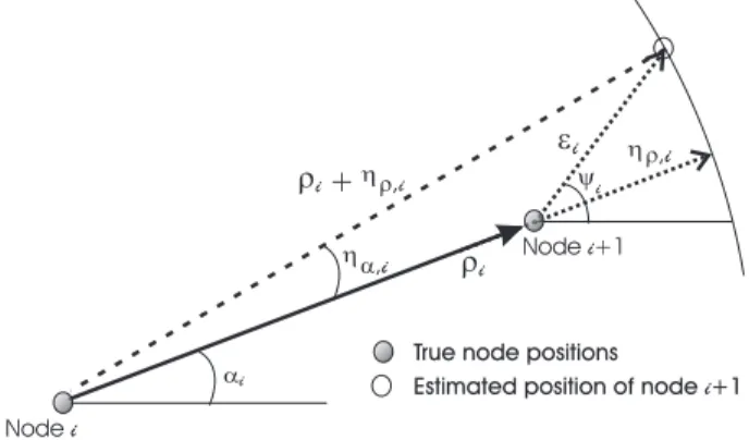
(33) 3.2. ERROR DISTRIBUTION OF THE DR SCHEME. 3.2. 15. Error Distribution of the DR scheme. First let us characterize the position estimation of a specific node of interest with unknown coordinates (x∗ , y ∗ ) using a single Dead Reckoning Path (DRP) between an AP with known coordinates (x0 , y0 ) and that node (see Figures 3.1 and 3.2). The intermediate nodes that link the node of interest with the AP conform the M hops of the DRP. The coordinates of these intermediate nodes will be denoted as (xi , yi ), i = 1...M . The true range and angle of the node of interest with respect to the AP can be represented by the vector addition p=. M X. bi ,. (3.1). i=1. where p and bi are vectors described by the magnitude-angle pairs (d, θ), and (ρi , αi ) respectively (see Section 3.1), and ρi =. p. (xi − xi−1 )2 + (yi − yi−1 )2 ,. αi = tan. −1. ³. yi −yi−1 xi −xi−1. (3.2). ´ ,. for i = 1, . . . , M . It should be clear that, at the M -th hop of the DRP, the link between the AP and the node of interest has been completed and hence xM = x∗ and yM = y ∗ . For the problem of interest, the Euclidean distances and angles defined in (3.2) are not available and can only be estimated at each hop. Therefore, to account for estimation errors we define the location vector observation as p̂ =. M X i=1. bi +. M X. ei ,. (3.3). i=1. where vector ei , which is described by the magnitude-angle pairs (²i , ψi ), i = 1, ..., M , corresponds to the measurement error vector at the i-th hop of the DRP (see Figures 3.1 and 3.2). It is easy to show that at the i-th hop 2 1/2 ²i = {2ρi [1 − cos(ηα,i )][ρi + ηρ,i ] + ηρ,i } ,. (3.4). and · ψi = π + αi − cos. −1. ρi − (ρi + ηρ,i ) cos(ηα,i ) ²i. ¸ .. (3.5). Hence, the error vector at the i-th hop, ei , depends on the ranging and AOA estimation errors ηρ,i and ηα,i respectively, and on the angular spread (relative angle) between the nodes conforming the i-th hop denoted as αi . (see Figures 3.1 and 3.2).

(34) 16. CHAPTER 3. MODEL DESCRIPTION. For the case where nodes are uniformly distributed within the network area, angular spread αi may be accurately modeled as a random variable symmetrically distributed 2 around zero degrees with variance σspread . High node density in the network and optimum routing algorithms that follow minimum distance criteria (see [32] and references therein) will tend to minimize this variance. Typical range estimation methods rely on the measurement of the line-of-sight (LOS) arrival time using a multipath power delay profile. Methods to measure multipath power delay profiles involve the transmission of a wide band PN-sequence with a chip rate equal to 1 Hz, and subsequent correlation of the received signal with this sequence (PN-correlation Tc methods). A subset of the local extrema of the correlator magnitude square are usually selected as the multipath delays and the first largest-magnitude delay is chosen as the LOS arrival. PN-correlation methods usually provide resolution to within Tc seconds. Due to this limited resolution, multipath that arrive less than Tc seconds after the LOS arrival time may add-up destructively and attenuate the magnitude of the LOS arrival. In this scenario, a contiguous subsequent strongest non-LOS arrival will be chosen as the first time of arrival and this in turn will translate in range estimation errors. It has been widely accepted that multipath interarrival times follow an exponential distribution (see [33] and references therein). Hence, ranging estimation errors caused by choosing contiguous subsequent non-LOS delays as first TOA estimates may also be considered exponential. Further, if we consider a homogenous environment (i.e. an environment where range and angular error statistics are the same for all the DRP hops) then the ranging estimation errors ηρ,i (i = 1...M ) may be modeled as exponential i.i.d. random variables with parameter λ whose inverse 1/λ corresponds to the average range estimation error at each hop. Angular errors ηα,i (i = 1...M ) will depend on the accuracy of the AOA estimators, these errors may be assumed random and symmetrically distributed around zero degrees with variance ση2α . Our interest is to statistically characterize the magnitude of the vector estimate p̂ given by ¯¯ ¯¯ M M ¯¯ ¯¯X X ¯¯ ¯¯ bi + ei ¯¯ , ||p̂||2 = r = ¯¯ ¯¯ ¯¯ i=1. i=1. (3.6). 2. where || · ||2 is the norm L2 . Following our assumptions, equations (3.4) and (3.5) show that if the angular spread 2 = 0) then ²i = ηρ,i and ψi = 0, in and AOA error variances equal zero (i.e. ση2α = σspread this case ranging errors are colinear to vectors bi , so ||p̂||2 = r = d + η , where the distance P d is given by d = M i=1 ρi and the ranging error η becomes a sum of M i.i.d. exponential random variables with parameter λ given by.

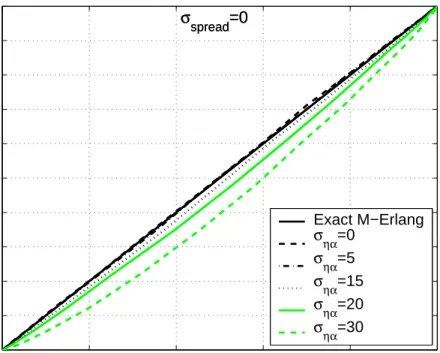
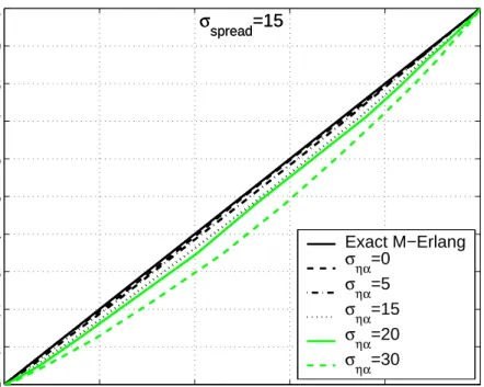
(35) 3.2. ERROR DISTRIBUTION OF THE DR SCHEME. η=. M X. ηρ i. 17. (3.7). i=1. It is well known that this sum is distributed as a M-Erlang random variable with parameter (λ) [34]. We have shown that in the most simplified scenario (perfect AOA estimation and zero angular spread α) the resultant DR magnitude estimation errors are M-Erlang distributed, but, what happens when the angular spread and AOA error variances depart from zero? We 2 claim that for certain values of ση2α 6= 0, σspread 6= 0, η may still be closely approximated as a M-Erlang random variable with parameter (λ). To support this claim 10,000 realizations of resultant DRP magnitudes were simulated assuming Gaussian angular spreads with zero mean and different standard deviations σspread values, Gaussian AOA estimation errors with zero mean and different standard deviation σηα values, M = 10 hops, and exponentially i.i.d. range estimation errors with parameter λ = 1. The Gaussian angular realizations mentioned above were truncated to 90 degrees for the case of angular spread and to 45 degrees for the case of AOA estimation errors in order to avoid impractical scenarios where the routing algorithm would link two nodes in a direction opposite to that of the node of interest and where an AOA estimation error would induce a negative ranging error η. Normalized histograms of the DRP magnitude error realizations were compared to the exact M-Erlang(λ) density function using probability-probability plots (PP-plots) shown in Figures 3.3, 3.4, 3.5 and 3.6. These figures show that the PP-plots for cases where σspread and σηα are smaller than 20 degrees are very close to the exact M-Erlang(λ) distribution. Furthermore we used the Kolmogorov-Smirnov goodness of fit test(often called the K-S test) that is used to determine whether two underlying probability distributions differ, or whether an underlying probability distribution differs from a hypothesized distribution, in either case based on finite samples. The K-S test is one of the most useful and general nonparametric methods for comparing two samples, as it is sensitive to differences in both location and shape of the empirical cumulative distribution functions of the two samples [38]. Figures 3.7 and 3.8 provides the results of the test of the normalized histograms of the DRP magnitude error realizations previously described versus a exact M-Erlang distribution with parameters M = 3, λ = 1 and M = 10, λ = 1 respectively. In Figures 3.7 and 3.8 when a zero value is displayed means that the null hypothesis was accepted (F (x) = F ∗ (x) for all x from −∞ to ∞), otherwise the null hypothesis was rejected. From these test and simulations was concluded that, as long as the angular spread and AOA estimation error standard deviations are less than 20 degrees, DRP magnitude errors η may be closely modeled as M-Erlang random variables with parameter (λ). As mentioned earlier, sufficient node density in the network and the implementation of shortest-distance.

(36) 18. CHAPTER 3. MODEL DESCRIPTION. 1. σspread=0. 0.9 0.8 0.7 0.6 0.5 0.4. Exact M−Erlang σ =0 ηα σ =5 ηα σ =15 ηα σηα=20 σηα=30. 0.3 0.2 0.1 0 0. 0.2. 0.4. 0.6. 0.8. 1. Figure 3.3: PP-plots to compare the exact M-Erlang(λ) density, σspread = 0, M = 10. 1. σspread=5. 0.9 0.8 0.7 0.6 0.5 0.4. Exact M−Erlang σ =0 ηα σηα=5 σηα=15 σηα=20 σηα=30. 0.3 0.2 0.1 0 0. 0.2. 0.4. 0.6. 0.8. 1. Figure 3.4: PP-plots to compare the exact M-Erlang(λ) density, σspread = 5, M = 10.

(37) 3.2. ERROR DISTRIBUTION OF THE DR SCHEME. 1. 19. σspread=15. 0.9 0.8 0.7 0.6 0.5 0.4. Exact M−Erlang σ =0 ηα σ =5 ηα σ =15 ηα σηα=20 σηα=30. 0.3 0.2 0.1 0 0. 0.2. 0.4. 0.6. 0.8. 1. Figure 3.5: PP-plots to compare the exact M-Erlang(λ) density, σspread = 15, M = 10. 1. σspread=30. 0.9 0.8 0.7 0.6 0.5 0.4. Exact M−Erlang σ =0 ηα σηα=5 σηα=15 σηα=20 σηα=30. 0.3 0.2 0.1 0 0. 0.2. 0.4. 0.6. 0.8. 1. Figure 3.6: PP-plots to compare the exact M-Erlang(λ) density, σspread = 30, M = 10.

(38) 20. CHAPTER 3. MODEL DESCRIPTION. Kolmogorov−Smirnov Test, M=3,. 1 0.8 0.6 0.4 0.2 0 30 30. 20 20 10. 10 0. σ. 0. ση. spread. α. Figure 3.7: Kolmogorov-Smirnov test versus σspread and σηα , M = 3 Kolmogorov−Smirnov Test, M=10,. 1 0.8 0.6 0.4 0.2 0 30 30. 20 20 10 σ. spread. 10 0. 0. ση. α. Figure 3.8: Kolmogorov-Smirnov test versus σspread and σηα , M = 10.

(39) 3.2. ERROR DISTRIBUTION OF THE DR SCHEME. 21. routing algorithms as well as high resolution array processing algorithms or antennas with large directivity may keep the angular spread and AOA estimation errors well within the allowable ranges. So let us now consider N ≥ 3 DRP position vector estimates. If we ignore the resultant vector angle θ at each of the N DRPs, the position of a node of interest may be estimated by applying a multilateration algorithm based on N observations that contain true distances corrupted by additive M-Erlang distributed noise. Define a vector containing the true coordinates of the node of interest as q = [x∗ y ∗ ]T . Let us now assume that N > 3 APs, with coordinates {xAP,i , yAP,i }, i = 1, . . . N , are available in the network and that the i-th AP establishes a link to the node of interest via Mi hops. As mentioned before, in this scenario we can obtain N noisy range measurements that are M-Erlang distributed. The i-th range observation may be denoted as ri = di (q) + ηi ,. (3.8). 1. where di (q) = [(xAP,i −x∗ )2 +(yAP,i −y ∗ )2 ] 2 is the true Euclidean distance between the unknown node position and the i-th AP (the dependence on the vector of true coordinates q has been emphasized). The error component ηi is M-Erlang distributed with parameter (λ). The M-Erlang density is given by the following equation fη (η) =. λ(λη)M −1 exp(−λη) , (M − 1)!. (3.9). Where M is always known (e.g. nodes may increment a counter in a data frame) whereas parameter λ is possibly unknown (and hence becomes a nuisance parameter). Notice that as λ grows, the error variance decreases. This parameter is the same for all the DRPs due to the assumption of homogeneity in the environment. Let us collect the N distance measurements in a vector to obtain r = d(q) + η ,. (3.10). where r = [r1 r2 ...rN ]T , d(q) = [d1 (q) d2 (q)...dN (q)]T and η = [η1 η2 ...ηN ]T . In this work it will be assumed that noise samples ηi and ηj (i 6= j) are independent. However it is important to emphasize that they are not identically distributed unless all the DRPs have the same number of hops. The independence assumption will be reasonable whenever the measured distances come from DRPs originating at sufficiently separated APs. Following the independence assumption, the joint distribution of the range observations is given by f (r ; θ) =. N Y λ{λ[ri − di (q)]}Mi −1 i=1. (Mi − 1)!. exp(−λ[ri − di (q)]) ,. (3.11).

(40) 22. CHAPTER 3. MODEL DESCRIPTION. Finally from 3.11, the log-likelihood function of the vector of observations r can be obtained as P L(r ; θ) = N i=1 − ln(Mi − 1)! + Mi ln λ +(Mi − 1) ln[ri − di (q)] − λ[ri − di (q)] .. 3.3. (3.12). Position Estimators. In this section we are going to propose a ML position estimation scheme assuming we have distance observations coming from N DRPs with a log-likelihood function given in equation (3.14).. 3.3.1. Maximum Likelihood Estimators. The maximum likelihood (ML) estimator chooses a position vector and a value of λ to maximize equation (3.14). This equation is highly non-linear and the ML estimator can not be found in closed form. However, we can solve the exact ML problem using the damped Newton-Raphson (NR) algorithm [35]. Specifically, we maximize (3.14) using the following recursion ". ∂ 2 L(r ; θ̂(n)) θ̂(n + 1) = θ̂(n) − γ(n) ∂θ∂θT. #−1. ∂L(r ; θ̂(n)) , ∂θ. (3.13). where θ̂ is the estimate vector given by θ̂ = [x̂ ŷ λ̂] and the damping factor γ(n) is chosen at every step to ensure that the log-likelihood function (3.14) increases and that the parameter estimates remain in the allowable parameter space. We will refer to this Newton Raphson - maximum likelihood algorithm as NR-ML. The gradient vector ∂L(r ; θ̂(n))/∂θ and the Hessian matrix ∂ 2 L(r ; θ̂(n))/∂θ∂θT have dimensions of 3×1 and 3×3 respectively and their derivatives can be computed as follows P L(r ; θ) = N i=1 − ln(Mi − 1)! + Mi ln λ +(Mi − 1) ln[ri − di (q)] − λ[ri − di (q)] .. (3.14).

(41) 3.3. POSITION ESTIMATORS. ∂L(r ; θ) ∂x. =. ∂L(r ; θ) ∂y. =. ∂L(r ; θ) ∂λ. =. 23. PN. 0. PN. 0. h. i=1 di,x. h. i=1 di,y. PN. ∂ 2 L(r ; θ) ∂x2. =. ∂ 2 L(r ; θ) ∂y 2. =. ∂ 2 L(r ; θ) ∂λ2. =. ∂ 2 L(r ; θ) ∂x∂y. =. ∂ 2 L(r ; θ) ∂x∂λ. =. ∂ 2 L(r ; θ) ∂y∂λ. =. Mi i=1 λ. PN. 1−Mi ri −di (q). h. di,x. PN. 00. h. i=1 di,y. PN i=1. PN PN. i +λ. i. 0. h. + λ + (di,x ). 1−Mi ri −di (q). i h i 0 1−Mi + λ + (di,y )2 (ri −d 2 i (q)). 2. 1−Mi (ri −di (q))2. i. 1−Mi ri −di (q). (3.15). i −M λ2. 00. i=1. i +λ. − (ri − di (q)). 00. i=1. 1−Mi ri −di (q). di,x,y. h. 1−Mi ri −di (q). i. 0. 0. + λ + di,x di,y. h. 1−Mi (ri −di (q))2. i. 0. i=1. PN. di,x 0. i=1. di,y. where 0. x−xAP,i di (q). 0. y−yAP,i di (q). 00. 1 di (q). −. (x−xAP,i )2 di (q)3. 1 di (q). −. (y−yAP,i )2 di (q)3. di,x = di,y = di,x = 00. di,y = 00. di,x,y = −. (3.16). (x−xAP,i )(y−yAP,i ) di (q)3. If the value of λ is known a priori, then the dimensions of the gradient and Hessian matrix are reduced by one since the derivatives with respect to λ can be ignored..

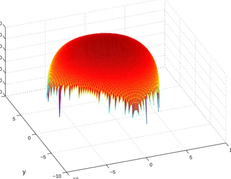
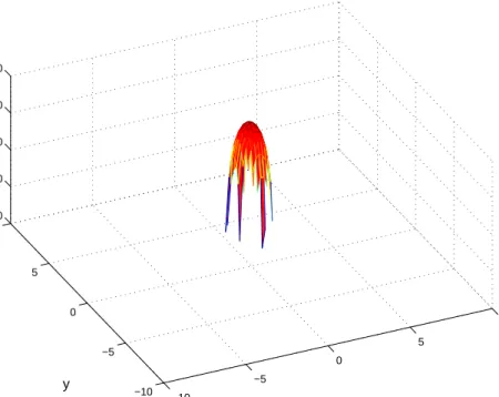
(42) 24. 3.3.2. CHAPTER 3. MODEL DESCRIPTION. Initialization of the NR-ML Algorithm. The NR recursion in (3.13) requires the choice of an initial parameter vector estimate θ̂(0). Showing that the likelihood functions are convex is not straightforward so we relied on plots of these functions to analyze convergence of the NR-ML algorithm. Figures 3.9 and 3.10 shows two examples of likelihood function surfaces versus coordinates x and y for the case where N = 9 APs. Both surfaces were obtained for true parameter values of λtrue = 1, and ∗ λtrue = 8 respectively. The true node position coordinates were set to x∗true = 0, ytrue =0 and the number of hops M = 10. Likelihood function versus x and y. −20 −40 −60 −80 −100 −120 −140 10. 5. 0 10 −5. 5 0. y. −10. −5 −10. x. ∗ Figure 3.9: Likelihood function versus x and y, N = 9, x∗true = 0, ytrue = 0, λtrue =1, M = 10.. It can be observed from both figures that there exists no local extrema that may damage the convergence of the algorithm. However, although only one global maximum exists, the surfaces become undefined (and equal to −∞) as x and y depart from the true ∗ = 0. It is then clear that for the NR-ML algorithm coordinate values x∗true = 0, ytrue to converge, initial coordinate values should be relatively close to the true ones. This necessity can be easily satisfied with a simple triangulation between three or more of the total N available DRP range measurements. It is worth noting from Figure 3.10 that as the error parameter λ increases, the likelihood surfaces become narrower suggesting that initial conditions should be chosen closer to the true coordinate values to avoid instabilities in the NR-ML recursions. Recalling that larger λ values yield smaller error variances (as reflected.

(43) 3.3. POSITION ESTIMATORS. 25. Likelihood function versus x and y. 0 −20 −40 −60 −80 10. 5. 0 10 5 −5. y. 0 −5 −10. −10. x. ∗ Figure 3.10: Likelihood function versus x and y, N = 9, x∗true = 0, ytrue = 0, λtrue =8, M = 10.. by the spikier likelihood surface), then triangulation should always yield sufficiently close initial coordinate values for any λ. Figure 3.11 shows the likelihood function versus λ for three different values of the true parameter λtrue . It is clear from these figures that there always exists only one global maximum and that the likelihood function exists for any value of λ. This means that convergence of the NR-ML algorithm will not be strongly affected by the initial value λ̂(0). Hence, if no prior knowledge is available about this parameter, λ̂(0) = 0 is a good initialization value.. 3.3.3. Least Squares Estimators. In order to compare the proposed NR-ML algorithm with classical multilateration techniques, this section summarizes the LWLS position estimation algorithm presented in [1]. If we assume that λ is known, the vector of unknown parameters becomes θ = q = ∗ ∗ T [x y ] . Then, the weighted least squares (WLS) estimator for θ can be found by minimizing the following functional P (r ; θ) = (r − d(q) − µ)T K−1 (r − d(q) − µ) , where µ = [ Mλ1 .... MN T ] λ. 1 and K = diag{[ M ... λ2. MN T ] }. λ2. (3.17).

(44) 26. CHAPTER 3. MODEL DESCRIPTION. Likelihood function vs. λ 0. −100. −200. −300. −400. −500 λ=6 λ=3 λ=1 1. −600 0. 2. 3. 4. 5 λ. 6. 7. 8. 9. 10. ∗ Figure 3.11: Likelihood function versus λ , N = 9, x∗true = 0, ytrue = 0, M = 10.. A simple closed form estimator is difficult to obtain due to the non-linearity of the functional in equation (3.17). To overcome this problem it is possible to linearize the functional by expanding the distance metric d(q) in a first order Taylor series around a known position vector q0 . It will be assumed that the value q0 is sufficiently close to the true position vector q so that the series expansion is an accurate approximation. The linearized distance metric can be written as dl (q) = d(q0 ) + D(q − q0 ) ,. (3.18). where D is a N × 2 matrix given by . 0. d1,y |q=q0 0 d2,y |q=q0 .. .. 0. dN,y |q=q0. dN,x |q=q0 0. 0. d1,x |q=q0  d0 |q=q 0  2,x D= ..  ..     , . (3.19). 0. 0. and di,x and di,y are defined in equation (3.16) in Appendix A. Using this linearized model we obtain the LWLS algorithm that obtains position estimates recursively using q̂(n + 1) = q̂(n) + (DT K−1 D)−1 DT K−1 [r − d(q̂(n)) − µ] .. (3.20).

(45) 3.3. POSITION ESTIMATORS. 27. It has been observed that this recursion converges even when the initial q̂(0) value is far from the true position vector q, [1]. Finally, it is easy to show, that the LWLS estimator is biased and has an error covariance matrix given by C = E{[q̂ − E{q̂}][q̂ − E{q̂}]T }} = (DT K−1 D)−1 ,. (3.21). The bias is non-zero due to the linearization of the distance metric and the covariance of this estimator is dependent on both the covariance matrix of the distance observations K and the linearization matrix D. Notice that in the case of Gaussian distributed distance observations, the LWLS estimator becomes the ML estimator for the linearized distance model. Apart from the statistical optimality differences between LWLS and NR-ML algorithms, notice that the latter does not require the linearization of the distance metric and hence solves an exact ML problem. In the following chapter will be shown (using computer simulations) that NR-ML is unbiased and asymptotically efficient.. 3.3.4. Cramer-Rao Bound for Position Estimators. The CRB provides a means for calculating a lower bound on the covariance of any unbiased location estimator that uses RSS, TOA, or AOA measurements. Such a lower bound provides a useful tool for researchers and system designers. Without testing particular estimation algorithms, a designer can quickly find the “best-case“ using particular measurement technologies. Researchers who are testing localization algorithms, can use the CRB as a benchmark for a particular algorithm. If the bound is nearly achieved, then there is little reason to continue working to improve that algorithmś accuracy. Furthermore, the bound‘s functional dependence on particular parameters helps to provide insight into the behavior of cooperative localization. The bound on estimator covariance is a function of the following:. 1. Number of unknown-location and known-location nodes. 2. Network geometry. 3. Whether localization is in two or three dimensions. 4. Measurement type implemented (RSS, TOA, or AOA). 5. Channel parameters. 6. Network connectivity..

(46) 28. CHAPTER 3. MODEL DESCRIPTION. 7. Nuisance (unknown) parameters that must be estimated. The bound is very similar to sensitivity analysis, applied to random measurements. The CRB is based on the curvature of the log-likelihood function. Intuitively, if the curvature of the log-likelihood function is very sharp like the right surface in Figure 3.9 , then the optimal parameter estimate can be accurately identified. Conversely, if the log-likelihood is broad with small curvature like the left surface in Figure 3.9 , then estimating the optimal point will be more difficult. The CRB is limited to unbiased estimators. Such estimators provide coordinate estimates that, if averaged over enough realizations, are equal to the true coordinates. Although unbiased estimation is a very desirable property, some bias might be tolerated to reduce variance. The CRB matrix for the unknown parameter vector θ can be computed by inverting the expected value of the negative Hessian matrix presented in 3.20, where the expectation is performed with respect to the distribution of the observation vector r. Then ½ · 2 ¸¾−1 ∂ L(r ; θ) . CRB(θ) = − E ∂θ∂θT. (3.22). It is difficult to obtain a closed form expression of the expectation in (3.22), however, the CRB can be calculated numerically by averaging the negative of the Hessian matrix over many realizations of r..

(47) Chapter 4 Numerical Results In this chapter several computer simulations are presented to demonstrate that the proposed NR-ML estimator is an unbiased estimator and hence is possible to measure its performance using the CRB, furthermore to analyze the effects of the average range estimation errors at each hop 1/λ, the number of hops M and the number of APs N on the accuracy of the NR-ML algorithm. We will also analyze the sensitivity of the position estimates to the knowledge of the nuisance parameter λ. Finally, we will compare NR-ML to the LWLS algorithm.. 4.1. Simulation Scenario Description. It has been assumed throughout the simulations that all the DRPs originating at N different APs have the same number of hops M . This is done for simplicity in presenting results, however it is important to emphasize that the proposed NR-ML algorithm is valid for the case where each DRP has a different M . Unless otherwise indicated, the simulations consider M = 10 hops at each DRP and that the node of interest is located at the center of a circle (coordinates (0, 0)) of maximum radius Rmax = 10. In all cases it is assumed that the APs are exactly located on the perimeter of the circle at equispaced angles and that all nodes in the network lie within this circle. Estimation of the position vector q and of parameter λ was simulated using the observation r for 3 ≤ N ≤ 30 APs. Ten thousand trials were performed at each point to ensure accurate estimates of bias and Mean Square Error (MSE). Numerical averaging (over observation r) of the Hessian matrix in (3.13) was also performed to calculate the CRB for estimates of q and λ using equation (3.22). Let us define the performance metrics used to present results. We define the normal2 . ized MSE for position estimates as E{||q − q̂||2 }/Rmax The normalization with respect to Rmax is done to ensure that the performance metric is independent of the dimensions of the area where all the network nodes exist and that 29.

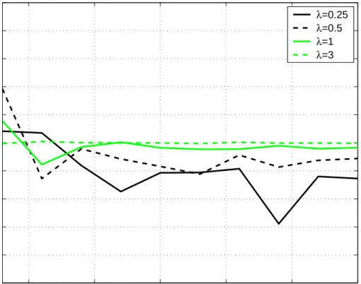
(48) 30. CHAPTER 4. NUMERICAL RESULTS. it solely reflects the effects of number of hops and λ. Next we find the normalized CRB 2 for position estimates as [CRB(x) + CRB(y)]/Rmax . Finally, the MSE for estimates of 2 parameter λ is simply given by E[(λ − λ̂) ].. 4.2. Bias of the NR-ML estimator. Here we are going to analyze the bias of the proposed NR-ML estimator, the bias of the position estimates in the x and y direction is defined as follows, E{x̂ − x∗ } and E{ŷ − y ∗ }. It was observed in all the simulations that the proposed NR-ML estimator is closely an unbiased estimator for λ = 0.25 and is clearly an unbiased estimator for the rest of the λ values. Figure 4.1 shows the bias of the x parameter estimate of position versus the number of APs for the case when λ is known and for values of λ = {0.25, 0.5, 1, 3} and as we can see the bias is always near to zero and it deteriorates as λ decreases (e.g., the best bias performance is shown when λ = 3). In Figure 4.2 shows the bias of the y parameter estimate of position versus the number of APs for the case when λ is known and for values of λ = {0.25, 0.5, 1, 3}, here we have the same performance as the one described above. Bias of estimates of x for different λ values 1. λ=0.25 λ=0.5 λ=1 λ=3. 0.8 0.6. Bias of estimates of x. 0.4 0.2 0. −0.2 −0.4 −0.6 −0.8 −1. 5. 10. 15 20 number of APs. 25. 30. Figure 4.1: Bias of estimates of x (E{x̂ − x∗ }) for different λ values..

(49) 4.2. BIAS OF THE NR-ML ESTIMATOR. 31. Bias of estimates of y for different λ values 1. λ=0.25 λ=0.5 λ=1 λ=3. 0.8 0.6. Bias of estimates of y. 0.4 0.2 0. −0.2 −0.4 −0.6 −0.8 −1. 5. 10. 15 20 number of APs. 25. 30. Figure 4.2: Bias of estimates of y (E{ŷ − y ∗ }) for different λ values..

(50) 32. 4.3. CHAPTER 4. NUMERICAL RESULTS. MSE and CRB of the NR-ML estimator. Let us now analyze the MSE performance of NR-ML. Figures 4.3 and 4.4 show the normalized MSE and normalized CRB for the estimates of position versus the number of APs for the cases where λ is known and unknown respectively for values of λ = {0.25, 0.5, 1, 3} in both figures. As expected, the performance of the estimator deteriorates as λ decreases. However, notice that in all cases the estimator is statistically efficient for sufficiently large values of N . Actually, for the cases where λ is known the normalized MSE and CRB are practically superimposed over all N . Normalized CRB and MSE for estimates of position, λ known Normalized MSE λ known Normalized CRB λ known 0. 10. Normalized MSE. λ=0.25. λ=0.5. −1. 10. λ=1 −2. 10. λ=3. 5. 10. 15 20 number of APs. 25. 30. Figure 4.3: Normalized MSE and CRB for position estimates when λ is known. Figures 4.5 and 4.6 show the normalized MSE and normalized CRB for the estimates of position versus the number of APs for the cases where λ is known and unknown respectively for values of λ = {0.25, 0.5, 1, 3}, but the main difference in these figures is that the number of hops was changed to M = 3. As expected, the performance of the estimator deteriorates as λ decreases. However, notice that in all cases the estimator is statistically efficient for sufficiently large values of N . Actually, for the cases where λ is known the normalized MSE and CRB are practically superimposed over all N as previosly shown in the Figures 4.3 and 4.4 in which the number of hops was M = 10..

(51) 4.3. MSE AND CRB OF THE NR-ML ESTIMATOR. 33. Normalized CRB and MSE for estimates of position, λ Unknown Normalized MSE λ Unknown Normalized CRB λ Unknown 0. 10. Normalized MSE. λ=0.25. λ=0.5. −1. 10. λ=1 −2. 10. λ=3. 5. 10. 15 20 number of APs. 25. 30. Figure 4.4: Normalized MSE and CRB for position estimates when λ is unknown..

(52) 34. CHAPTER 4. NUMERICAL RESULTS. Normalized CRB and MSE for estimates of position, M=3, λ known Normalized MSE λ known Normalized CRB λ known λ=0.25. −1. Normalized MSE. 10. λ=0.5. −2. 10. λ=1. −3. 10. λ=3. 5. 10. 15 20 number of APs. 25. 30. Figure 4.5: Normalized MSE and CRB for position estimates when λ is known, M = 3..

(53) 4.3. MSE AND CRB OF THE NR-ML ESTIMATOR. 35. Normalized CRB and MSE for estimates of position, M=3, λ Unknown Normalized MSE λ Unknown Normalized CRB λ Unknown. 0. 10. λ=0.25. −1. Normalized MSE. 10. λ=0.5 −2. 10. λ=1. −3. 10. λ=3. 5. 10. 15 20 number of APs. 25. 30. Figure 4.6: Normalized MSE and CRB for position estimates when λ is unknown, M = 3..

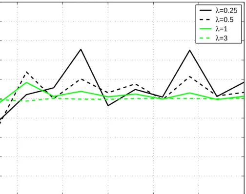
(54) 36. CHAPTER 4. NUMERICAL RESULTS. An important conclusion that can be obtained from these figures is that the proposed estimator is quite insensitive to the knowledge of the nuissance parameter λ. For large enough N the normalized MSE and CRB curves are practically the same for the cases where λ is known (Figure 4.3) and the cases where this nuisance parameter is unknown (Figure 4.4). It can be concluded that for large values of N knowledge of parameter λ will not improve the estimation performance of the algorithm. Figure 4.7 presents the normalized MSE for position estimates versus the number of APs for the case where λ = 1 and for different number of hops conforming the DRPs. As expected, the performance of the estimator deteriorates as the number of hops M increases since the variance of the observations increases with M . Normalized MSE vs. number of APs for different number of hops, λ=1 M=3 M=10 M=20 M=30 −1. Normalized MSE. 10. −2. 10. 5. 10. 15 20 number of APs. 25. 30. Figure 4.7: Normalized MSE for position estimates for different number of hops M . The results presented in Figures 4.3, 4.4 and 4.7 were obtained assuming that the node of interest is positioned at the center of a circle of radius Rmax . Let us now analyze the effects of moving the node of interest away from the center of the circle. To do this we obtained 500 realizations of the normalized MSE curves for estimates of position as the ones presented in Figure 4.3 and 4.4. Each of the 500 normalized MSE curve realizations was obtained using a random and uniformly distributed set of coordinates for the node of 2 where 0 < υ < 1 is a constant used to ensure that interest in the region x2 + y 2 < υRmax.

(55) 4.4. NR-ML VERSUS LWLS ESTIMATORS RESULTS. 37. the nodes will be positioned at least one average hop-size away from any AP and, with this, avoid ambiguities. The number of hops at each DRP was kept constant and equal to M = 10 regardless of the random position of the node of interest. The average of the 500 realizations of the normalized MSE curves is presented in Figure 4.8 together with the normalized MSE curve for the case where the node of interest is centered at (0, 0). These results were obtained for λ = {0.25, 0.5, 1} and using υ = 0.8. Average Normalized MSE for uniformly distributed node positions 0. Mean Normalized MSE (random positions) Normalized MSE Pos=(0,0). 10. Normalized MSE. λ=0.25. λ=0.5. −1. 10. λ=1. −2. 10. 5. 10. 15. 20. 25. 30. number of APs. Figure 4.8: Expected value of normalized MSE From Figure 4.8 we observe that the curves obtained in the case where the node of interest is centered at (0, 0) are upper bounds to the average performance for cases where the node of interest is located at any random point in the network. Further, as the value of λ increases these upper bounds become tighter.. 4.4. NR-ML versus LWLS estimators results. In this eection we are going to analyze the performance of the NR-ML algorithm for the SE estimation of λ. Figure 4.9 shows efficiency ( M ) curves for estimates of λ and for values CRB.

(56) 38. CHAPTER 4. NUMERICAL RESULTS. of λ = {0.25, 0.5, 1, 3} versus the number of APs. It is observed that in all cases the efficiency becomes close to one for sufficiently large N . Estimation efficiency for λ 1 0.9 0.8. Efficiency. 0.7 0.6 0.5 0.4 0.3 0.2. λ=0.25 λ=0.5 λ=1 λ=3. 0.1 0. 5. 10. 15 20 number of APs. 25. 30. Figure 4.9: Efficiency curves for estimates of λ. The estimation of λ becomes less efficient as its true value decreases. Large values of N will be necessary to accurately estimate small values of λ. For example, more than 30 APs will be necessary to achieve 80% efficiency when λ = 0.25. On the other hand, 3 APs are enough to achieve more than 80% efficiency in the case where λ = 3. Let us now compare the performance of the NR-ML algorithm with respect to the performance of LWLS for the case where λ is known. Results were calculated for different number of APs and for different values of λ and are presented in Figure 4.10 in the form of normalized MSE for position estimates. It can be seen that NR-ML outperforms LWLS in all the cases presented in this figure (λ = {0.25, 1, 3}). Moreover, since the normalized MSE results are presented on a logarithmic scale it is clear that this difference in performance increases as the variance of the observations becomes larger. The relative performance of LWLS versus NR-ML can be seen to be between 50 and 33 % for all values of λ and N . Apart from being statistically optimal, the better performance of NR-ML is due to the fact that this algorithm does not require the linearization of the distance metric and hence solves an exact ML problem..

(57) 4.4. NR-ML VERSUS LWLS ESTIMATORS RESULTS. 39. LWLS vs ML. 0. λ=0.25. −1. λ=1. −2. λ=3. Normalized MSE. 10. 10. 10. 5. 10. ML LWLS. 15 20 number of APs. 25. Figure 4.10: Performance of LWLS vs NR-ML.. 30.

(58) 40. CHAPTER 4. NUMERICAL RESULTS. All the results presented so far in this section have been calculated using resultant distance observations r that follow an exact M-Erlang (λ) distribution.. 4.5. Deviation from the M-Erlang model. This section will analyze how does the NR-ML algorithm becomes affected when resultant distance observations deviate from this exact M-Erlang distribution due to non-zero angular 2 spread and AOA estimation error variances (ση2α 6= 0, σspread 6= 0). Simulations were performed for Ad-Hoc network scenarios consisting of N = 10 APs exactly located at equispaced angles on the perimeter of a circle of radius Rmax = 10. Node density in the network was set to achieve an average of 10 hops per DRP and the node of interest was placed at the (0, 0) coordinate. DRP resultant distance observations r were simulated using different values of angular spread and AOA estimation standard deviations in the interval {σηα , σspread } ∈ [0, 40] degrees. A total of 5, 000 network realizations and position estimates were obtained for various combinations of σηα and σspread values. Figures 4.11 and 4.12 show the mean absolute deviation of the simulated normalized MSE results with respect to the normalized MSE results obtained with the exact M-Erlang (λ) observations for the cases where λ = 0.25 and λ = 1 respectively. These absolute deviations have been plotted versus the angular spread and AOA estimation error standard deviations. It is clear that as the angular spread and AOA estimation error standard deviations increase, the actual NR-ML results deviate further and further form the exact maximum likelihood results. However, notice that for values of {σηα , σspread } < 20 degrees the mean absolute deviation from the exact maximum likelihood problem will be less than 0.05 in the case where λ = 0.25 and less than 0.004 in the case where λ = 1. These deviations are fairly small and confirm that the exact M-Erlang approximation is acceptable as long as {σηα , and σspread } are relatively small. Recall that the 20 degree limit for the angular spread and AOA estimation standard deviations was obtained in Section 3.2 by analyzing the PP-plots presented in Figures 3.3, 3.4, 3.5 and 3.6..

(59) 4.5. DEVIATION FROM THE M-ERLANG MODEL. 41. Absolute deviation from exact M−Erlang normalized MSE, λ=0.25 0.18. 0.16. 0.2. 0.14. 0.15 0.12. 0.1. 0.1. 0.08. 0.05. 0.06. 0 40. 0.04. 40. 30 30. 20 10 σ. spread. 0.02. 20 10 0. 0. 0. σ. η. α. Figure 4.11: Mean absolute deviation of simulated normalized MSE results, M = 10..

(60) 42. CHAPTER 4. NUMERICAL RESULTS. Absolute deviation from exact M−Erlang normalized MSE, λ=1. −3. x 10 12. 10. 0.014 0.012 0.01. 8. 0.008 0.006. 6. 0.004 0.002. 4. 0 40 40. 30 30. 20. 20. 10 σ. spread. 2. 10 0. 0. σ. η. α. Figure 4.12: Mean absolute deviation of simulated normalized MSE results, M = 10..