Evolutionary prototype selection for multi output regression

(1)

Contents lists available at ScienceDirect

Neurocomputing

journal homepage: www.elsevier.com/locate/neucom

Evolutionary

prototype

selection

for

multi-output

regression

Mirosław

Kordos

b

_,

_Álvar

_{Arnaiz-González}

a

_,

_César

_{García-Osorio}

a, ∗

a_Department_of_Civil_Engineering,_University_of_Burgos,_Spain

b_Department_of_Computer_Science_and_Automatics,_University_of_{Bielsko-Biala,}_Poland

a

r

t

i

c

l

e

i

n

f

o

Articlehistory: Received19July2018 Revised5March2019 Accepted23May2019 Availableonline24May2019

CommunicatedbyProf.ZidongWang

Keywords: Prototypeselection Multi-output Multi-target Regression

a

b

s

t

r

a

c

t

A novel approach toprototype selection for multi-output regression datasets is presented. A multi-objectiveevolutionaryalgorithmisusedtoevaluatetheselectionsusingtwocriteria:trainingdataset compressionandpredictionqualityexpressedintermsofrootmeansquarederror.Amulti-target regres-sorbasedonk-NNwasusedforthatpurposeduringthetrainingtoevaluatetheerror,whilethetests wereperformedusingfourdifferentmulti-targetpredictivemodels.Thedistancematricesusedbythe multi-target regressorwerecached toaccelerateoperationalperformance.Multiple Pareto frontswere alsousedtopreventoverﬁttingandtoobtainabroaderrangeofsolutions,byusingdifferent probabil-itiesintheinitializationofpopulationsanddifferentevolutionaryparametersineachone.Theresults obtainedwiththebenchmarkdatasetsshowedthattheproposedmethodgreatlyreduceddatasetsize and,atthesametime,improvedthepredictivecapabilitiesofthemulti-outputregressorstrainedonthe reduceddataset.

1. Introduction

Machine Learning uses data sets for learning tasks, that con- sist of collections of observations and historical data. Each element of a data set is an instance that comprises a series of attributes: the input attributes that have to be measured for new observations; and, the output attributes that will be predicted. Tradition- ally, interest has mainly been focused on a single output attribute, which can either be nominal, for classiﬁcation problems, or continuous for regression problems. Recent research has also focused on the simultaneous prediction of several target attributes. In this case, we refer to multi-label problems when considering nominal attributes [1], and we refer to multi-output regression problems when predicting continuous attributes [2].

1.1. Prototype selection

An important part of the Machine Learning pipeline is the initial data pre-processing step. Prototype selection (or instance selection) is one of the tasks at that stage. The ﬁrst purpose of prototype selection is to obtain a reduced data set that can be used to train predictive models successfully with a similar performance to

∗ _{Corresponding}_author.

E-mail addresses: mkordos@ath.bielsko.pl (M. Kordos), alvarag@ubu.es (Á. Arnaiz-González),cgosorio@ubu.es(C.García-Osorio).

those that can be obtained using the whole data set [3]. In some cases, this reduction simply attempts to remove outliers and noisy instances, thereby facilitating the learning of a model and even improving its performance [4]. In others, the reduction is more ag- gressive, seeking the application of methods that might otherwise not be applied to the initial data set, and doing so without ex- cessively affecting the performance of such methods. The avail- ability of a reduced data set, that retains the properties of the original one, also permits several methods to be tested within a reasonable time, or to try several parameter values of a method to ﬁnd the best model to solve the prediction task. Obviously, this task is much more challenging in multi-output regression than in single-label classiﬁcation or in traditional (single-output) regression.

There are plenty of prototype selection methods for classiﬁca- tion problems, for a thorough review of prototype selection methods, we recommend the taxonomy of Garcia et al. [5]. Over the past few years, some of these algorithms have been adapted to deal with regression problems [6,7]. It has also recently become possible to perform instance selection with extremely large data sets using algorithms of linear complexity [8] and implementations that exploit the parallelization of the map-reduce approach [9,10]. Unfortunately, there are only a few prototype selection methods for multi-label classiﬁcation [11] and, to the best of our knowledge, there are as yet no prototype selection methods for multi-output regression. Thus, the aim of this paper is twofold:

https://doi.org/10.1016/j.neucom.2019.05.055

(2)

• To propose the ﬁrst prototype selection method that is capable of dealing with multi-output regression data sets (EPS-MOR). The method consists of several stages and uses the multi- objective evolutionary algorithm NSGA-II [12] as the engine that searches the solution space.

• To evaluate the performance of the EPS-MOR algorithm in an experimental study that thoroughly investigates the performance of the proposal, verifying not only the possibility of greatly reducing the size of the data sets, but also of improving the multi-output predictive capacity of the models trained with the reduced set.

The paper will be organized as follows: in Section2, the concept of multi-output regression will be introduced; the instance selection task will be presented in Section 3 along with its aims and diﬃculties; in Section4, the EPS-MOR algorithm is explained; then, the experimental setup and the results will be presented and analyzed in Section5; ﬁnally, the main conclusions will be sum- marized in Section6.

2. Multi-outputregression

Multi-output regression, also known as multivariate or multi- target regression, is a task that involves the prediction of multiple continuous values by using a set of input variables or features [13] (so the problem is also multivariable). Consider a training set D =

{

(

x1,y1

)

,...,

(

xn ,yn

)

}

with n instances, each of them composed of d descriptive attributes and q target variables. Formally, a multi-target regression problem can be deﬁned as the task of learning a model h : X→Y, where X⊆Rd _{is a set of input} attributes, and _Y_⊆_Rq consists of a set of target variables that, given an unlabeled input instance x, can predict its output set of variables [14,15].

A simple approach to multi-output regression would be to consider each of the outputs to be predicted as independent, and to learn a different model for each of them (commonly known as the single-target method). However, this procedure was incapable of exploiting the existing relationships between the different outputs. In fact, the models that exploit those relationships have proven that they can give much better results than those obtained by independent models [2,16,17]. Two strategies are commonly considered for dealing with multi-label/multi-output data sets: data transformation and algorithm adaptation [2]. The former is mainly based on transforming the multi-output label data set into a set of single-target data sets, which are then used for training a model for each target. The prediction is made by concatenating the different predictions of each regressor. In this work, we used four data- transformation methods implemented in Mulan [18]:

• Single-target regressor: the equivalent of the binary relevance method [19] for regression. Binary relevance creates as many single-label data sets as there are labels in the original multi- label data set. A classiﬁer is then trained with each of these sets. Single-target regressors perform in the same way, but a regressor instead of a classiﬁer is trained.

• Multi-target stacking: inspired by the stacked binary relevance technique, adapts the idea of stacked generalization [20] to multi-label learning. It consists of two stages: in the ﬁrst stage, as many independent models as outputs are trained (as in single-target); these models are used to generate meta- variables for use at a later stage. The second stage builds the same number of models as the previous stage, but the original instances are augmented by the estimation of the values of their target attributes.

• Regressor chain: inspired by the classic classiﬁer chains method [21]. Several regressors are chained in sequence, the

first learns the relation between the inputs and the first output, the second uses the inputs and the output of the first to learn the second output,...: the last regression model attempts to predict the last output using all the inputs and all the outputs predicted by the previous regressors. The drawback of this method is that it is highly affected by the order in which the outputs are sorted in the chain.

• An ensemble of regressor chains serves to mitigate the inﬂu- ence of the order in the chaining order, by combining several regressor chains with different chaining orders in an ensemble.

3. Prototypeselectionandstate-of-the-art

The task of selecting a subset of a large number of instances, examples or points, that are able to preserve the predictive capabilities of the entire set is an important and well-known problem in Machine Learning. These elements, that are able to summarize the whole data set, are called prototypes, representatives, or exemplars.

3.1. Prototype selection for single-label/output data

Prototype selection, also known as instance selection [5], is the task of selecting the most relevant instances/prototypes/examples from a data set. The aim of these algorithms is to obtain a subset of the original data set with the same (or in certain cases even higher) predictive capabilities than the original set [22]. In other words, given a training set, T , the problem is to select a subset S ⊆T , so that S contains no irrelevant or superﬂuous instances, and so that the accuracy of a predictor trained with S is similar to the results of having used T [23] (or even better if the prototype selection method is capable of removing those instances that com- plicate the learning task, such as noise and anomalies).

Prototype selection is a multi-objective problem [24]: both accuracy and compression are important. A properly performed instance selection ﬁrst removes noise and then compresses the remaining data. At the noise removal stage, both objectives can frequently be improved; removing the few noisy instances also lowers the RMSE and increases the compression. So, if the data set is more strongly compressed, improving compression worsen the RMSE , and the reverse.

The first prototype selection proposals for the nearest neighbor classifier date back to the late sixties and early seventies, where the two first methods, Condensed Nearest Neighbor [25] (CNN) and Edited Nearest Neighbour [26] (ENN), were proposed. Since then, a large number of different proposals have emerged. A detailed review of these methods is beyond the scope of the paper, although we recommend [5] to readers with an interest in those methods.

3.2. Subset representatives selection

The problem of ﬁnding a subset of representative examples that are able to summarize the whole data set has also been widely researched in such ﬁelds as computer vision, image processing, bioinformatics, and recommender systems, among others [27]. In these kinds of applications, the instances/examples are usually re- ferred to as representatives or exemplars [28].

(3)

The problem of ﬁnding data representatives has been broadly researched [29,31]. Although, as for prototype selection, a thorough review of these methods is not the aim of this paper.

3.3. Evolutionary methods of prototype selection

Evolutionary algorithms make no assumptions about data set properties. Instead, they empirically verify large numbers of different subsets in an intelligent way to minimize the search in the solution space. This approach frequently yields much more efficient solutions than those that are achievable with non-evolutionary methods. Regarding prototype selection, evolutionary algorithms have shown better results than other approaches to the problem [32,33]. On the other hand, the good results usually imply much higher computational cost. Below, we briefly review the application of some evolutionary algorithms for instance selection for single-label classification tasks that can be found in the literature.

The first proposals of evolutionary instance selection methods were based on the application of conventional evolutionary search algorithms to the selection of prototypes [34,35]. Tolvi [36] used genetic algorithms for outlier detection and variable selection in linear regression models, performing both operations simulta- neously. In [37], an algorithm called Cooperative Coevolutionary Instance Selection (CCIS) was presented. The method used two populations that were evolved cooperatively. The training set was divided into approximately N equal parts, and for each part a subpopulation of the first population was used. Each individual in a subpopulation encoded a subset of training instances. Like- wise, each subpopulation was evolved using a standard genetic algorithm for its evolution. The second population consisted of combinations of instance sets. The population of individuals kept track of the best combinations of selectors for different subsets of instances, yielding a final selection that had the most promising combination for the whole data set.

Antonelli et al. [38] presented a complex genetic algorithm for dealing with prototype selection. They tackled the problem through a co-evolutionary approach in the framework of multi- objective evolutionary fuzzy systems. During the execution of the learning process, a genetic algorithm periodically evolved a population of reduced training sets. The single-objective algorithm aims to optimize an index that measures how close the results obtained with the reduced set are from those obtained when using the whole data set.

To the best of our knowledge, there are only three papers that describe the application of multi-objective evolutionary algorithms for prototype selection. All of them have been published in the last two years and were designed for single-label classiﬁcation problems.

In [39], the MOEA/D algorithm was used to integrate instance selection, instance weighting, and feature weighting. The paper was focused on the use of co-evolution to approach the simultaneous selection of instances and hyper-parameters to train an SVM. The optimization criteria were the reduction of the training set and the performance (when the reduced set was used to train an SVM with the hyper-parameters found for the algorithm).

Another interesting approach is the one proposed by Escalante et al. [40], consisting in updating the training and validation parti- tions at each iteration of the genetic algorithm, in order to prevent the prototypes from overﬁtting a single validation data set.

In [41] Acampora et al. proposed a multi-objective training set selection. Their algorithm was mainly based on the evolutionary algorithm PESA-II [42] and was used for improving the performance of SVM by proper training set selection. They included several modiﬁcation in their design for improving the performance of the PESA-II as a prototype selection algorithm.

Table1 shows a comparison between the method proposed in this paper (EPS-MOR) and all the aforementioned algorithms.

3.4. Prototype selection for multi-output data

Even though prototype selection has been broadly researched for single-label classiﬁcation and, to a lesser degree, for single- output regression; the same can not be said for multi-label/multi- output [11]. In the same way as classiﬁer or regressor adaptation to multi-output, two approaches can be used for adapting single-label prototype selection methods to multi-output scenarios: data transformation (i.e. transform original multi-output data sets on one or more single-label data sets) and method adaptation (i.e. adapt the original single-label prototype selection methods, so that they can process multi-output data sets). Data transformation techniques for prototype selection were studied in [11]. Regarding method adaptation, there are currently only three prototype selection algorithms capable of processing multi-label data sets:

• Charte et al. [43] proposed a heuristic undersampling method for imbalanced multi-label data sets based on the canonical Wilson Editing method [26].

• Kanj et al. [44] proposed a prototype selection method, also based on Wilson Editing, that aims to purify the data set by removing harmful instances.

• Arnaiz-González et al. [45] recently proposed a method for adapting the local-set concept, successfully used on single-label instance selection methods [24,46], to multi-label data sets. It was used for adapting two single-label instance selection methods, LSSm and LSBo, to multi-label learning.

To the best of our knowledge, there are no prototype selection algorithms capable of processing multi-output regression data sets. So, up until now, it has not been possible to exploit the advantages offered by the prototype selection methods for this kind of problem: namely the speeding up of model learning, by means of data set size, and the performance increase of the trained models, as a consequence of the reduction of noisy and anomalous instances.

The challenges of prototype selection for multi-output data sets are manifold. One is related to the diﬃculties associated with prototype selection for regression [6] (it is usually diﬃcult for the prototype selection algorithms for regression to improve the predictive capabilities of the methods trained with the selected subset [7]), and the other is related to the problems that arise when prototype selection is applied to multi-label data sets [43].

4. Evolutionaryprototypeselectionformulti-outputregression (EPS-MOR)

In this section, EPS-MOR, the proposed evolutionary method of prototype selection for multi-output regression is presented. The aim of EPS-MOR is to obtain several possible reduced training sets, which minimize two criteria: the training set size and the prediction error of a model trained on the reduced data set. Our method uses as a search algorithm a multi-objective genetic algorithm based on NSGA-II as a search algorithm to ﬁnd the optimal solutions. The ﬁrst criterion (compression) is just the ratio between the size of the selected subset and the size of the original set. The second criterion is the prediction error on the test set, which during the prototype selection process is approximated by the prediction error on the training set, because the output values of the test set instances are normally unknown just before the training starts.

Some characteristics of EPS-MOR worth highlighting are:

• For the ﬁrst time, a prototype selection for multi-output regression is presented.

(4)

Table1

Comparisonbetweentheproposedmethodandseveralevolutionaryinstanceselectionalgorithms.Foreachmethodthetableshowsthetypeofdata settowhichisapplied(single-labelormulti-output),thetypeoffunctionisoptimizing(single-objectiveorbi-objective),theevolutionaryalgorithm usedforthesearch,thetypeofcrossoverandmutationoperators,andifitusesParetofronts,howtheyareused.

Algorithm Label Objective Evol.algorithm Crossover Mutation Paretofront

CHC[35] Single-label Single-objective CHC Single-point -

-GGA[34] Single-label Single-objective - Single-point Symmetric -CCIS[37] Single-label Single-objective - Two-point Symmetric -Tolvi[36] Single-output Single-objective - Single-point Symmetric -PAES-SOGA[38] Single-output Single-objective (2+2)M-PAES Single-point Symmetric

-EMOMIS[39] Single-label Bi-objective MOEA/D Single-point Symmetric Ensemblecombination MOPG[40] Single-label Bi-objective NSGA-II Multi-point Symmetric Highestaccuracy Pareto-TSS[41] Single-label Bi-objective PESA-II Single-point Asymmetric Summodel EPS-MOR Multi-output Bi-objective NSGA-II Multi-point Asymmetric 3-frontcombination

• Use of up to three populations with different initialization and mutation probabilities. These three can be merged into a single Pareto front, in order to reduce overﬁtting and improve cover- age of the solution space.

• Use of asymmetric mutation: making it possible to have data sets with lower error in the populations.

• Eﬃcient evaluation of the ﬁtness function by pre-calculating and reusing the distances matrices for k -NN (calculated and sorted only once at the beginning of the process).

In the following sections more details are given of certain relevant steps of the method.

4.1. Basic concepts of evolutionary prototype selection

Prototype selection is a bi-objective task with two goals: min- imization of the number of instances in the training set (compression) and maximization of the prediction quality of the model trained on the selected instances [24]. In the case of the regression task, the prediction quality is commonly measured by using the mean squared error on the test set.

Each individual in the population represents a set of selected instances. Every single position in the individual chromosome represents an instance of the training data set. A value of 1 at a given position means that the corresponding instance is selected and a value of 0 means that is rejected.

In standard (single-objective) genetic algorithms used for prototype selection, both objectives are incorporated into a single ﬁtness function, which measures the quality of the obtained solution. One of the simplest versions of a ﬁtness function is shown in Eq.(1):

ﬁtness=

γ

avgRMSE_rmse +

(

1−

γ

)

avgN_numInstancesumInstances

p (1)

where, the RMSE is the root mean square error of the model trained on the current training set, avgRMSE is the average RMSE over the whole population of training sets, numInstances is the number of selected instances in the current training set, and avgN- umInstances is the average number of selected instances over the whole population of training sets.

γ

is a value between 0 and 1 that controls the importance given to each of the objectives. p is a positive real number, controlling the steepness of the ﬁtness functions, i.e. how much the better solutions are favored.

As may be deduced, the most time-consuming part of the genetic algorithm is the evaluation of the ﬁtness function value, as it requires a calculation of the RMSE performed by the predictive model on the training set. (In the method that is presented, special effort was spent on reducing this time, as will be discussed later.)

There are two problems with the single-objective approach. First, we must know which weights to assign to each criterion. Second, if we need several solutions with different weights, then the optimization needs to be run several times: each time with a

different

γ

value ( Eq.(1)) to achieve one solution, which is deﬁ- nitely a time-consuming process.

4.2. Multi-objective genetic algorithms for prototype selection

The main advantage of multi-objective evolutionary algorithms is that they do not require the coeﬃcients that indicate the expected balance between the objectives (

γ

value of Eq.(1)) to be determined. Instead, these algorithms produce a set of solutions that generate the highest ﬁtness, i.e. the result of the algorithm is the front of the non-dominated individuals (Pareto front) with different trade-offs between objectives. Solutions based on Pareto- front and domination between individuals [47] can be divided into ranking, elitist and diversity maintaining methods [48].

A solution x dominates another solution y (with the minimiza- tion goal) if it achieves better (lower) or equal values of all objective functions (of all criteria), and additionally better value of at least one objective function (one criterion) [49], this is when both equations below are satisﬁed:

ob ji

(

x

)

≤ob ji

(

y

)

for alli

ob j_i

(

x

)

< ob j_i

(

y

)

for at leastonei (2)

where i is the objective function index ( i = 1 ...O ), O is the number of objectives, and obj _i(...) is the objective function. The examples of domination between individuals and the Pareto front can be seen in Fig.2.

Despite the fact that several multi-objective evolutionary algorithms have been proposed [12], the NSGA-II algorithm is the most frequently used and one of the best for bi-objective problems. (For more than two objetives, there is an extension of the aforementioned algorithm called NSGA-III [50]).

4.3. Genetic operators

Seeking to obtain the best results for the prototype selection problem, several improvements to the genetic operators were introduced, as explained below.

4.3.1. Crossover

(5)

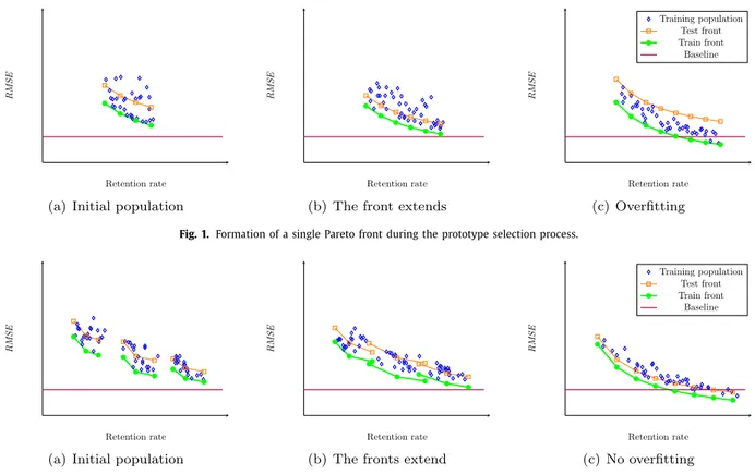
Fig.1. FormationofasingleParetofrontduringtheprototypeselectionprocess.

Fig.2. FormationofaParetofrontusingthreesub-frontsduringtheprototypeselectionprocess.

effectively the highly ﬁtted blocks in the chromosome, as their construction will be permanently disrupted. Experimentally, we derived the formula shown in Eq. (3), explained later at the end of Section5.2.

4.3.2. Mutation

There are cases where a genetic algorithm can find the optimal solutions even without the mutation operator. For example, when the chromosome is short enough and the population is large enough. However, in other cases the mutation operator is crucial, especially in the final stages of the process, where the diversity of the population is limited and some optimal positions in the chromosome may no longer exist in any individual. (Or even if they do exist, the individual may have low fitness and therefore a low probability of selection as a parent for the next generation.)

Commonly, in evolutionary algorithms, a symmetric mutation operator is used, i.e. the probability of switching from 1 to 0 is the same as from 0 to 1. The problem that arises is that symmetric mutation exerts a pressure on the process to set, on average, the same number of ones and zeros as in the initial population. That problem is also one of the reasons why the multi-objective prototype selection genetic algorithms tend to contract the Pareto front, not including the solutions that have selected either very few or too many instances.

In the problem of prototype selection, we are not interested in extreme data set reduction, if it is at the cost of worsening the error too much (which will make the selection useless in real applications, as the subset would not be representative of the original data set, leaving it of no use for learning tasks). We are interested in reductions that keep the statistical properties of the original data set, but allowing predictors with lower errors and good generalization to be obtained.

In some data sets, the lowest error is obtained when quite a lot of instances are rejected, say 40% or 50%. In that case, there is no problem and the symmetric mutation will do properly.

Nonetheless, for other data sets obtaining the lowest error requires rejecting very few instances, frequently below 10%. In these cases, we should enforce those solutions will be found by generating the initial population with much more ones than zeros in the chromosome and using the asymmetrical mutation operator to maintain this proportion as the process progresses. Thus, for example the probability of switching from 0 to 1 can be 90%, while the probability of switching from 1 to 0 will be 10%.

4.4. Extending the Pareto front

In a typical optimization process, where the genetic algorithm directly optimizes the ﬁnal objectives, a simple approach to ﬁnd the best possible solution is to increase the number of iterations. Nevertheless, prototype selection belongs to a different class of problems, because the optimization is performed on the training set (the test set is unknown during the optimization), yet one of the objectives is to reduce the RMSE in the test. For this reason, the RMSE on the training set is minimized during prototype selection, assuming that it yields a decrease of the RMSE on the test set.

It is similar to the process of training a predictive model. Anal- ogously, as we cannot train the model for too many iterations, we cannot run the genetic optimization too long, because overﬁtting begins to occur at a certain point; the RMSE is constantly decreas- ing on the training set, but at a certain point it begins to increase in the test set. The simplest solution to this problem is to use early stopping, which in our preliminary experiments worked well in more than half of the data sets.

For explanatory purposes, let us consider the idealized situa- tion shown in Figs.1 and 2. At the beginning of the optimization, all positions in all chromosomes have random values. Thus, the lo- cations of all the individuals 1 _{in the compression-}_{RMSE space are}

(6)

very close to each other and they all have a relatively poorly bal- anced compression- RMSE for any

γ

value in Eq. (1). These loca- tions are shown in Fig.1 (a), where the blue diamonds represent the solutions of the evolutionary algorithm. Each solution (set of selected instances) on the Pareto front of the training set is used to train a model. The green circles (connected with the thick line) represent the RMSE value obtained from the regressor that was in turn trained using the selected subset applied to the training subset itself. Obviously, this RMSE is a very optimistic estimation of the error as the same data set is used both for training and testing. The result of the model on the test set is expected to be higher and, in the ﬁgures, it is represented by an orange square just above the green circle (both marks: the orange square and the green circle are obtained from the same training set of selected instances, hence they have the same compression value — the compression of the selected training set). As the green circles, the orange squares are connected by a line, although this time a thin one that represents the expected Pareto front on testing. The baseline represented by the horizontal line is the RMSE on the training set obtained by the regressor trained on the original full size data set.

As the optimization progresses, the points move gradually to the positions shown in Fig.1 (b), and then 1 (c). But, before they reach the positions in Fig.1 (c), the overﬁtting has already started to happen (the green thick line in Fig. 1 (c) is lower than in Fig.1 (b), and the thin orange line is situated at a higher point, i.e. more RMSE ).

Nonetheless, as shown in Fig.2 (c), when there are more fronts, solutions with low compression and low RMSE are reached before overﬁtting occurs. (The thick green line in Fig.2 (c) is lower than in Fig.2 (b), and the thin orange line is also lower).

Frequently we do not need the front to be extended in the di- rection of low compression (high retention rate), because the lowest RMSE is already reached below the baseline in Fig.1 (b) and will probably not improve any further. However, if the lowest RMSE is at or above the baseline, we may want to search for a solution with an even lower RMSE . Running the optimization for more iterations will not always lower the RMSE , as it will also cause overfitting. We therefore need to obtain more fronts, which we call sub-fronts, to cover a broader space without overfitting. The sub- fronts are obtained by generating the initial populations with different proportions of 0 and 1, and then, using different probabilities in the mutation phase, so that the percentage of 0s and 1s in the chromosomes remain relatively close to the proportions in the initial populations, as it is shown in Fig.2 (a). Finally, the sub- fronts will be merged into one Pareto front (and thus some points from some sub-front may not be included in the final front, if the points from another sub-front satisfy both objectives with greater accuracy).

4.5. Summary of EPS-MOR

In summary, the sequence of steps of the proposed method is:

1. Calculate and sort the distance matrices that will be used later by k -NN based predictive models.

2. Obtain the Pareto front of the selected test sets:

(a) Initialize the population P with S individuals, with different proportions of 0s and 1s in each front.

(b) Start the iterative prototype selection process:

i. Evaluate the population P according to the two objec- tives: compression and average RMSE .

ii. Select the individuals that will be included in each of the fronts. First, the non-dominated individuals from P populations are transferred to the ﬁrst front. Then, the next front is selected from remaining individuals. This process

Table2

Summaryofdatasetscharacteristics:name,domain,numberofinstances,features, andtargets.

Datasets Domain Instances Attributes Targets

Num. Nom.

Andromeda Water 49 30 0 6

Slump Concrete 103 7 0 3

EDM Machining 154 16 0 2

ATP7D Forecast 296 211 0 6

Solarﬂare1 Forecast 323 0 10 3

ATP1D Forecast 337 411 0 6

Jura Geology 359 15 0 3

Onlinesales Forecast 639 401 0 12

ENB Buildings 768 8 0 2

Waterquality Biology 1060 14 0 16

Solarﬂare2 Forecast 1066 0 10 3

SCPF Forecast 1137 23 0 3

Riverﬂow1 Forecast 9125 64 0 8

performance is optimized by Fast Non-dominated Sort (for further details see [12]).

iii. Calculate crowding distances. Within each front a crowding distance for each individual is calculated (for further details see [12]). It determines the distance between neighboring individuals from a given front and promotes more diverse solutions in the following selection process. iv. Apply the multi-point multi-parent crossover. In this step a population P with s children is created. For each child, a number of parents is chosen using ranking selection (using values speciﬁc to each front and then crowding distance — individuals with smaller values are selected). v. Apply the mutation operator with probabilities speciﬁc

to each front.

vi. Merge the populations. Populations P and P are merged into a single one ( P =P ∪P ).

vii. Select the individuals that will be included in the com- bined front and calculate the crowding distances for the merged population P .

viii. From the population P (with size 2 ·s ) s best individuals are selected. In this selection, the individuals from the front are prioritized. If the front has less than s individuals, all of them are included and the rest, up to s , are randomly selected from the rest of individuals of population P not in the front. If in the front there are already more than s individuals, only the s with largest crowding distance are selected.

ix. Evaluate the stopping criterion. The algorithm stops if the criterion is met, otherwise the algorithm will perform the next iteration.

(c) Return, as the result of the prototype selection process, the ﬁrst front of non-dominated solutions with all the solutions found (each of them represents a reduced data set). 3. Check whether the next front is required: if so, go to point 2a. 4. Merge all fronts into one ﬁnal front of solutions.

5. Experimentalevaluation

The performance of EPS-MOR was experimentally evaluated in a 10-fold cross-validation process using several multi-output regressors and compared with the results of training the regressors using the original data sets. The software was written in C# language for performing the prototype selection process, and Mulan [18] was used to evaluate the results. The experiments were performed on the 13 multi-output regression data sets (see Table2) that are the benchmark ﬁles available from the Mulan project website 2_{. All the}

(7)

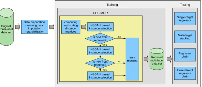
Fig.3. Thegraphicalrepresentationoftheexperimentalprocess.

software and data sets used in the experiments can be downloaded from http://kordos.com/eps-mor.

5.1. Experimental setup

The experimental setup is presented in Fig.3. First of all, two additional pre-processing steps were performed: missing data imputation (replacing missing values by the mean of the feature), and nominal attribute replacement (transforming them into binary ones) 3_.

During training, the distance matrices were ﬁrstly computed and sorted. Then the NGSA-II algorithm was used for searching the solution space. Initially, the population was randomly gener- ated with a 0.5 probability of 0 and 1 at each position, equal to the probability of either selecting or rejecting each instance (if needed, the next two sub-fronts were obtained, with different proportions of 0s and 1s, and all the sub-fronts merged into the ﬁnal Pareto front).

In the testing part, the base regressor was k -NN ( k = 1 _,3 _,5 ) adapted to multi-output regression by four different techniques [14]: single-target regressor, multi-target stacking, regressor chain, and ensemble of regressor chains. All of the parameters of the regressors were set to the default values in Mulan. The average root mean squared error ( RMSE ) was used as a measure of the prediction quality:

RMSE=1 q

q

j=1

n

i =1

y_{i j}−yˆ_{i j}2 n

where, n is the number of instances, q the number of outputs, y i and ˆ y _iare, respectively, the vector of the actual and the predicted outputs for x_i.

In a typical case, Fig. 4 shows the Pareto front obtained in training (green circles), some of the solutions of this front (orange squares) and their positions in testing, and a horizontal line repre- senting the error obtained by the regressor trained with the whole data set. As can be seen, the solutions that ﬁnd themselves exactly on the Pareto front in training are displaced when the testing error is considered (although their compression is exactly the same,

3_Both_the_missing_data_imputation_and_nominal_to_binary_features_replacement wereperformedbyusingWeka[51].

Fig.4. Schematicrepresentationofthedifferent instanceselectionsolutions se-lectedforthe experimentalcomparisons.Baselinerepresentsthe RMSEobtained withthetestsetoftheregressortrainedontheoriginaltrainingdataset.

their RMSE can differ). However, it is expected that most of them will be close enough to the ideal Pareto front in testing (some exceptions are mentioned in the discussion of the experiments).

The results of a multi-objective evolutionary algorithm simulta- neously yield several solutions. These results are always advanta- geous, since one could then either choose solutions with higher compression, or solutions with a lower error, depending on the speciﬁc needs of the problem to solve (as discussed later on, the high cost, traditionally associated with genetic algorithms, is not so high, if they are carefully implemented). Nevertheless, to facili- tate the analysis of the experimental results, only 3 representative solutions were considered:

• EPS-MOR-1st: The ﬁrst point of the Pareto Front, i.e., the solution with the lowest compression and with the lowest RMSE on the training set. Although it is not guaranteed that this subset will produce the lowest RMSE on the training set in every case, it will usually do so.

(8)

Table3

Summaryoftheparameters’valuesofEPS-MORusedintheexperiments.

Parameter Value

Numberofepochs 25

Numberofindividuals 96

Numberofparentsandcrossoverpoints givenbyEq.(3)

Initializationprobability 0.5(1st_front),_0.8₍₂nd_front),_0.92₍₃rd_front) Mutationprobability(1st_front) _0.005_from₁_to₀_and_from₀_to₁ Mutationprobability(2nd_front) _0.002_from₁_to₀_and_0.008_from₀_to₁ Mutationprobability(3rd_front) _0.001_from₁_to₀_and_0.009_from₀_to₁ Crossoverprobability 100%

Innerregressor setofsingletargetk-NNregressors

Table4

SummaryoftheresultsfortheRMSEwithk-NNregressorwithk=1(lowerisbetter).Thebestresultforeachdataset(andregressor)andthebestvaluesare highlightedinbold.

(a)single-target (b)stackingofsingle-target

Dataset Original EPS-MOR Dataset Original EPS-MOR

1st bsl 5pc 1st bsl 5pc

Andromeda 0.4478 0.4419 0.4419 0.5151 Andromeda 0.4478 0.4419 0.4419 0.5151

SCPF 0.9580 0.7633 0.8556 0.8556 SCPF 0.9580 0.7633 0.8556 0.8556

Waterquality 0.9421 0.8944 0.9036 0.9036 Waterquality 0.9421 0.8944 0.9036 0.9036 Solarflare1 1.2250 0.8985 1.1894 1.2981 Solarflare1 1.2312 0.8988 1.1832 1.2923 Solarflare2 0.9353 0.8396 0.9193 0.9557 Solarflare2 0.9506 0.8389 0.9203 0.9558

Slump 0.9086 0.8031 0.8857 0.9468 Slump 0.9086 0.8031 0.8857 0.9468

ATP1D 0.5535 0.5151 0.4872 0.6966 ATP1D 0.5535 0.5151 0.4872 0.6966

ATP7D 0.7823 0.7342 0.7412 0.7844 ATP7D 0.7823 0.7342 0.7412 0.7844

EDM 0.6035 0.5252 0.5970 0.6718 EDM 0.6035 0.5252 0.5970 0.6718

Riverﬂow1 0.0901 0.0661 0.0786 0.0786 Riverﬂow1 0.0901 0.0661 0.0786 0.0786

ENB 0.5732 0.5257 0.4443 0.4443 ENB 0.5732 0.5257 0.4443 0.4443

Jura 0.8133 0.8059 0.8059 0.8577 Jura 0.8133 0.8059 0.8059 0.8577

Onlinesales 0.9003 0.8589 0.8956 0.9637 Onlinesales 0.9003 0.8589 0.8956 0.9637

Average 0.7487 0.6671 0.7112 0.7671 Average 0.7503 0.6670 0.7108 0.7666

(c)chainofk-NNregressors (d)ensembleofchains

Andromeda 0.4478 0.4419 0.4419 0.5151 Andromeda 0.4114 0.4912 0.4912 0.5555

SCPF 0.9580 0.7633 0.8556 0.8556 SCPF 0.8266 0.7453 0.7938 0.7938

Waterquality 0.9421 0.8944 0.9036 0.9036 Waterquality 0.8284 0.7983 0.8138 0.8138 Solarflare1 1.2525 0.8976 1.1832 1.2959 Solarflare1 1.1081 0.8928 1.0540 1.1344 Solarflare2 0.9799 0.8387 0.9193 0.9549 Solarflare2 0.9234 0.8164 0.8776 0.8831

Slump 0.9086 0.8031 0.8857 0.9468 Slump 0.7516 0.7861 0.8507 0.9070

ATP1D 0.5535 0.5151 0.4872 0.6966 ATP1D 0.4772 0.5555 0.5330 0.6893

ATP7D 0.7823 0.7342 0.7412 0.7844 ATP7D 0.6810 0.6702 0.7035 0.7051

EDM 0.6035 0.5252 0.5970 0.6718 EDM 0.5804 0.5228 0.6146 0.7409

ENB 0.5732 0.5257 0.4443 0.4443 ENB 0.4623 0.4175 0.3883 0.3883

Jura 0.8133 0.8059 0.8059 0.8577 Jura 0.7304 0.7431 0.7431 0.8020

Onlinesales 0.9003 0.8589 0.8956 0.9637 Onlinesales 0.7907 0.7786 0.8086 0.8781

Average 0.7542 0.6669 0.7107 0.7668 Average 0.6658 0.6372 0.6731 0.7207

regressor trained on the whole training set). This result would usually correspond to a solution with a RMSE that is close to the one obtained with the whole data set, but with higher compression than EPS-MOR-1st.

• EPS-MOR-5pc: The point of the Pareto front that shows a 5% higher RMSE on the test set than the ﬁrst solution (EPS-MOR- 1st). That solution has a worse RMSE , but with much more compression than EPS-MOR-1st.

At times, some of the solutions can actually be the same: for example, if the ﬁrst point is above the baseline, EPS-MOR-1st and EPS-MOR-bsl share the same RMSE . It is also possible that EPS- MOR-5pc might have a lower error than, for example, the error of the EPS-MOR-1st plus 5%, if the last point of the Pareto front is reached and its error is still not 5% higher than EPS-MOR-1st. Even in some cases, the ﬁrst point of the Pareto front has higher error than some of the next points and EPS-MOR-bsl could be even better than EPS-MOR-1st, for some data sets.

5.2. Parameters of the evolutionary prototype selection algorithm

An initial exploratory analysis was performed before the experiments, in order to select the best parameters for EPS-MOR. De- spite the fact that a carefully and customized parameter tuning for each data set could have achieved better results, we launched all the experiments with a common conﬁguration of parameters for all data sets. Table 3 shows the values of the parameters ﬁnally used, which are explained in greater detail below.

(9)

Table5

(a)Single-target (b)Stackingofsingle-target

Andromeda 0.5870 0.5066 0.5810 0.6491 Andromeda 0.5642 0.4663 0.5659 0.6078

SCPF 0.8430 0.7366 0.8224 0.8646 SCPF 0.8578 0.7356 0.8232 0.8650

Waterquality 0.7884 0.7804 0.7770 0.8103 Waterquality 0.7878 0.7853 0.7841 0.8356 Solarflare1 1.0279 0.9096 0.9897 0.9897 Solarflare1 1.0607 0.9086 0.9871 0.9871 Solarflare2 0.9072 0.8592 0.8772 0.8772 Solarflare2 0.9056 0.8684 0.8886 0.8886

Slump 0.7000 0.7398 0.7398 0.7694 Slump 0.6868 0.7708 0.7708 0.7793

ATP1D 0.4389 0.4577 0.4577 0.4698 ATP1D 0.4391 0.4580 0.4580 0.4702

ATP7D 0.6268 0.6360 0.6360 0.6643 ATP7D 0.6268 0.6361 0.6361 0.6644

EDM 0.5866 0.5833 0.5833 0.6190 EDM 0.5715 0.5806 0.5806 0.6165

ENB 0.2967 0.3049 0.3049 0.3117 ENB 0.2764 0.2965 0.2965 0.3039

Jura 0.7229 0.7273 0.7273 0.7713 Jura 0.7350 0.7385 0.7385 0.7739

Onlinesales 0.8001 0.8199 0.8199 0.8938 Onlinesales 0.7983 0.8240 0.8240 0.9016

Average 0.6476 0.6256 0.6454 0.6742 Average 0.6464 0.6263 0.6484 0.6746

Andromeda 0.5700 0.4976 0.5915 0.6409 Andromeda 0.5999 0.5285 0.6112 0.6620

SCPF 0.8333 0.7356 0.8188 0.8620 SCPF 0.7763 0.7370 0.7862 0.8181

Waterquality 0.7890 0.7871 0.7846 0.8074 Waterquality 0.7654 0.7653 0.7689 0.7945 Solarflare1 1.0187 0.9106 0.9824 0.9824 Solarflare1 1.0129 0.8924 0.9241 0.9241 Solarflare2 0.8876 0.8593 0.8858 0.8858 Solarflare2 0.9149 0.8517 0.8606 0.8606

Slump 0.7209 0.7508 0.7508 0.7786 Slump 0.7166 0.7249 0.7249 0.7588

ATP1D 0.4372 0.4577 0.4577 0.4695 ATP1D 0.4315 0.4449 0.4449 0.4659

ATP7D 0.6243 0.6343 0.6343 0.6608 ATP7D 0.6083 0.6066 0.6066 0.6232

EDM 0.5749 0.5833 0.5833 0.6107 EDM 0.6278 0.6161 0.6161 0.6773

ENB 0.2919 0.3089 0.3089 0.3187 ENB 0.3438 0.3253 0.3253 0.3499

Jura 0.7293 0.7239 0.7239 0.7733 Jura 0.7247 0.7270 0.7270 0.7749

Onlinesales 0.7943 0.8151 0.8151 0.8960 Onlinesales 0.7780 0.7824 0.7824 0.8874

Average 0.6434 0.6258 0.6471 0.6739 Average 0.6443 0.6212 0.6351 0.6673

• Population size: the optimal value slightly grows with the chromosome length, and it was about 60–70 for the data sets with less than 1 0 0 0 instances and around 75–85 for the larger ones. The difference in the optimization time, between 65 and 100 individuals, was about 3% – the function resembled a parabolic curve and grew very slowly close to the minimum (a very ﬂat parabola). Using only a single CPU, the time of the process is proportional to the number of ﬁtness function evalua- tions. Nonetheless, in multi-CPU solutions, the dependence is more complex and for optimal performance the population size should be a multiple of the available CPU core number. As we used a 48-core machine for the experiments, we set the population size at 96 individuals.

• Crossover: multi-point multi-parent crossover can signiﬁcantly increases the convergence on the genetic instance selection algorithm (a 3-fold increase in our experiments). The optimal number of parents can be equal to the optimal number of split points and both can be set, so on average the split occurs from every 10 positions for short chromosomes up to every 100 positions for longer chromosomes ( Eq.(3)). The parents were randomly selected with a probability proportional to their ﬁtness value. Each selection was independent, so it could happen that one parent was selected more than once, giving its genetic material to more than one segment of the child chromosome.

M=

_round

₍

_n_/₁₀

₎

_for _n_≤₁₀₀₀

100+round

(

n−1000

)

/ 100

)

for n > 1000 (3)

5.3. Results and discussion

Tables 4, 5, and 6 show the RMSE results of the k -NN clas- siﬁer ( k = 1 ,3 ,5 ) adapted to multi-label by means of: single target, multi-target stacking, chain of k -NN, and an ensemble of k -NN chains, with (EPS-MOR-1st, EPS-MOR-5p, EPS-MOR-bsl) and without prototype selection. Table 7 shows the compression rates (in percentages) achieved by EPS-MOR.

As shown in Tables 4, 5, 6 (a), the application of some data set size reduction algorithm (EPS-MOR-1st solutions) reduced the RMSE consistently in most data sets, as might be expected, given that prototype selection was very likely to remove outliers and noisy instances. The compression achieved by EPS-MOR-1st was re- markable, at around 40%, i.e. the 60% of instances were kept and the RMSE was lowered. However, applying more extreme reduction (EPS-MOR-5p solutions) rised the RMSE and the number of remaining instances may be insuﬃcient to train a model with suf- ﬁcient generalization. And between these two (EPS-MOR-bsl solutions), a RMSE slightly lower than the baseline was achieved, but with higher compression values than EPS-MOR-1st solutions.

It is worth noting the results of data sets ATP1D and ENB, where the EPS-MOR-bsl solution, despite applying a reduction higher than EPS-MOR-1st, managed to reduce the RMSE . This ef- fect could be explained because, although the solutions are from the Pareto front obtained in training, when the RMSE from the testing procedures was considered, the solutions themselves would not necessarily form a Pareto front.

(10)

Table6

(a)Single-target (b)Stackingofsingle-target

Andromeda 0.5870 0.6019 0.6019 0.6257 Andromeda 0.5642 0.5804 0.5804 0.6100

SCPF 0.7850 0.7311 0.7842 0.7971 SCPF 0.7898 0.7401 0.7850 0.7965

Waterquality 0.7704 0.7728 0.7728 0.7932 Waterquality 0.7734 0.7772 0.7772 0.8037 Solarflare1 0.9539 0.9044 0.9072 0.9633 Solarflare1 0.9892 0.9068 0.9186 0.9754 Solarflare2 0.8868 0.8423 0.8606 0.8606 Solarflare2 0.9058 0.8618 0.8739 0.8739

Slump 0.7121 0.7098 0.7098 0.7560 Slump 0.7153 0.7183 0.7183 0.7609

ATP1D 0.4435 0.4412 0.4412 0.4725 ATP1D 0.4425 0.4433 0.4433 0.4732

ATP7D 0.6104 0.6384 0.6384 0.6488 ATP7D 0.6103 0.6376 0.6376 0.6468

EDM 0.5812 0.5701 0.5701 0.6158 EDM 0.5841 0.5701 0.5701 0.6144

ENB 0.3123 0.3032 0.3065 0.3375 ENB 0.3110 0.2997 0.3076 0.3366

Jura 0.7229 0.7256 0.7256 0.7592 Jura 0.7350 0.7369 0.7369 0.7623

Onlinesales 0.8116 0.8018 0.8018 0.8603 Onlinesales 0.8050 0.8010 0.8010 0.8769

Average 0.6358 0.6245 0.6313 0.6602 Average 0.6390 0.6269 0.6337 0.6633

Andromeda 0.5700 0.6104 0.6104 0.6140 Andromeda 0.5999 0.6212 0.6212 0.6282

SCPF 0.7596 0.7280 0.7805 0.7854 SCPF 0.7374 0.7306 0.7540 0.7999

Waterquality 0.7763 0.7809 0.7809 0.7974 Waterquality 0.7627 0.7662 0.7662 0.7692 Solarflare1 0.9562 0.9065 0.9086 0.9569 Solarflare1 0.9481 0.9087 0.9049 0.9630 Solarflare2 0.8890 0.8459 0.8559 0.8559 Solarflare2 0.8943 0.8457 0.8458 0.8458

Slump 0.7273 0.7211 0.7211 0.7633 Slump 0.7060 0.7059 0.7059 0.7426

ATP1D 0.4422 0.4418 0.4418 0.4728 ATP1D 0.4322 0.4383 0.4383 0.4637

ATP7D 0.6096 0.6399 0.6399 0.6480 ATP7D 0.5999 0.6436 0.6436 0.6415

EDM 0.5840 0.5701 0.5701 0.6110 EDM 0.6344 0.6755 0.6755 0.6843

Riverﬂow1 0.0875 0.0757 0.0875 0.0919 Riverﬂow1 0.0791 0.0793 0.0940 0.0980

ENB 0.3091 0.3057 0.3072 0.3376 ENB 0.3189 0.3121 0.3252 0.3541

Jura 0.7293 0.7305 0.7305 0.7531 Jura 0.7247 0.7348 0.7348 0.7679

Onlinesales 0.8065 0.8001 0.8001 0.8499 Onlinesales 0.7817 0.7910 0.7910 0.8356

Average 0.6344 0.6274 0.6334 0.6567 Average 0.6322 0.6348 0.6385 0.6611

Table7

Summaryofthecompressionresults(inpercentage)oftheprototypeselectionmethod.

Dataset k=1 k=3 k=5

1st bsl 5pc 1st bsl 5pc 1st bsl 5pc

Andromeda 45.12 45.12 49.29 22.68 30.55 40.74 17.14 17.14 17.80

SCPF 67.99 82.39 82.39 67.16 83.18 86.35 67.62 75.20 94.14

Waterquality 51.32 80.86 80.86 62.41 66.21 80.31 9.84 9.84 81.08

Solarﬂare1 69.39 89.82 95.51 82.64 89.65 89.65 67.67 83.02 89.48

Solarﬂare2 69.55 82.46 82.97 66.47 78.85 78.85 72.49 82.85 82.85

Slump 56.73 78.85 80.05 54.14 54.14 56.31 19.61 19.61 63.73

ATP1D 49.29 52.30 59.94 49.31 49.31 60.15 10.68 10.68 57.91

ATP7D 60.68 77.78 79.67 6.18 6.18 59.62 54.95 54.95 56.24

EDM 41.69 64.92 67.76 31.96 31.96 52.29 40.46 40.46 46.62

Riverﬂow1 64.05 79.32 79.32 67.92 73.88 73.88 66.89 73.78 76.16

ENB 19.43 80.86 80.86 13.55 13.55 14.02 58.31 67.75 80.91

Jura 5.18 5.18 62.39 10.09 10.09 57.02 1.37 1.37 48.29

Onlinesales 9.93 44.71 51.29 5.52 5.52 62.17 10.33 10.33 70.36

Average 46.95 66.51 73.25 41.54 45.62 62.41 38.26 42.08 66.58

front for most training sets when the RMSE in the testing procedure was considered (except for data sets ATP1D and ENB mentioned as exceptions above).

The strategy of combining several regressors chains can be seen in subtables (d) of Tables4,5, and 6, corresponding to the regressor chain ensemble. As a robust ensemble method, the improvements introduced by prototype selection were hardly noticeable.

Table7 shows the compression rates (in percentages) achieved by EPS-MOR when k =1 , k =3 and k =5 are used. As expected, the best compression rates were achieved at the point EPS-MOR- 5pc (of the three selected solutions, which is towards the left) with an average compression rate of between 62 and 73% . Nevertheless, this high compression has as a counterpart high error rates, as has

previously been shown. It should be mentioned that EPS-MOR-1st (the most conservative solution) achieved both high compression rates, of around 38 −47% , and high accuracy expressed by a low RMSE .

5.3.1. Statistical tests

Average ranks [52] and the Hochberg procedure [53] were both computed for a proper comparison of the results. Table8 summa- rizes the results of the RMSE for each regressor and k value for k =1 , 3, and 5. The best method according to the RMSE is high- lighted in bold, and the symbol ( ✖) indicates that the result is sta- tistically worse than the best method in each block (at a level of

(11)

Table8

Averagerankingsforthedifferentregressorsandkvalues.Thebestresultsforeachregressorandkvaluearehighlightedinbold.Thesymbol(✖)markstheresults thatarestatisticallyworsethanthebestineachblock(atalevelofα=0.05).

kvalue Algorithm Single-target MTstacking k-NNchain Ensembleofchains

k=1 Original 3.3077✖ 3.3077✖ 3.3846✖ 2.5385

EPS-MOR-1st 1.3077 1.3077 1.3077 1.6145

EPS-MOR-bsl 1.9231 1.9231 1.9231 2.4615

EPS-MOR-5pc 3.4615✖ 3.4615✖ 3.3846✖ 3.3846✖

k=3 Original 2.3077 2.0769 2.2308 2.2308

EPS-MOR-1st 1.8077 1.8846 1.8077 1.5709

EPS-MOR-bsl 2.2308 2.3846 2.3077 2.4615

EPS-MOR-5pc 3.6538✖ 3.6538✖ 3.6538✖ 3.7308✖

k=5 Original 2.4615 2.1538 2.3846✖ 1.6923

EPS-MOR-1st 1.6154 1.7692 1.6154 2.0769

EPS-MOR-bsl 2.0385 2.2692 2.1154 2.5000

EPS-MOR-5pc 3.8846✖ 3.8077✖ 3.8846✖ 3.7308✖

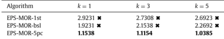
Table9

Averagerankingsofcompression.Thebestresultforeachregressorishighlighted inbold.Thesymbol(✖)markstheresultsthatarestatisticallyworsethanthebest (atalevelofα=0.05).

Algorithm k=1 k=3 k=5

EPS-MOR-1st 2.9231✖ 2.7308✖ 2.6923✖ EPS-MOR-bsl 1.9231✖ 2.1538✖ 2.2692✖

EPS-MOR-5pc 1.1538 1.1154 1.0385

Some remarks of interest in relation to Table9 are as follows:

• The subsets obtained with EPS-MOR-1st consistently yielded the best results in all situations, except in the case of the ensemble of chains of regressors at k ₌ 5 . As previously discussed, the robustness obtained by the ensemble and a high number of k had already yielded a very good result that would be diﬃcult to improve upon.

• If we focus on the value of the regressors with k = 1 , the solutions corresponding to EPS-MOR-1st were signiﬁcantly better than those obtained when using the whole data set, for all methods, except, once again, for the ensemble of chains of regressors, where it was better (but not signiﬁcantly).

• For all regressors and k values, EPS-MOR-1st was signiﬁcantly better than EPS-MOR-5pc. As commented earlier, the compression of EPS-MOR-5pc was too high and the highly reduced data sets were unable to retain the prediction capabilities of the whole data set.

Table9 shows the Average ranks and Hochberg procedures over compression. As expected, taking into account compression, the best results were achieved by EPS-MOR-5pc, followed by EPS-MOR- bsl and EPS-MOR-1st, in that order. Moreover, the differences between EPS-MOR-5pc and the other two were signiﬁcant (at a level of

α

=0 .05 ).

6. Conclusions

EPS-MOR has been presented as the first prototype selection method for multi-output regression problems. The bi-objective evolutionary algorithm NSGA-II has been used as the search algorithm for the prototype selection method. The design of EPS-MOR overcomes the limitations of the NSGA-II regarding overfitting by using, when needed, more than one Pareto front with specific initialization and mutation parameters, which were merged to obtain the final solutions. Also, to speed up the evaluation of the fitness function, the distances were pre-calculated and cached at the beginning of the execution.

The experimental validation of EPS-MOR has shown that despite the large reduction of data set size, in some cases by more than 50%, when the selected instances are used to train multi- output regressors, their performance is not worse and can even be better than having trained the regressors on the whole data set.

The performance and eﬃciency shown by EPS-MOR demon- strates that the Pareto-based multi-objective evolutionary approach can offer a good trade-off between compression and accuracy for multi-output regression tasks. One of its great advantages is that, instead of a single solution, many solutions are obtained from which one can be chosen. So, if greater importance is attached to the reduction of the RMSE , a solution on the right side of the Pareto front can be used. Otherwise, if the reduction of the data set size is being sought, a left side solution can be chosen.

Declarationofcompetinginterest

We declare that there is no conﬂict of interest.

Acknowledgements

This work was supported by the NCN (Polish National Sci- ence Center) grant “Evolutionary Methods in Data Selection ” No. 2017/01/X/ST6/00202, project TIN2015-67534-P (MINECO/FEDER, UE) of the Ministerio de Economía y Competitividad of the Spanish Government, and project BU085P17 (JCyL/FEDER, UE) of the Junta de Castilla y León coﬁnanced with European Union FEDER funds.

References

[1] G.Tsoumakas,I. Katakis,Multi-label classiﬁcation:anoverview,Int.J.Data Warehous.Mining3(3)(2007)1–13.

[2] H.Borchani,G.Varando,C.Bielza,P.Larrañaga,Asurveyonmulti-output re-gression,WileyInterdiscipl.Rev.:DataMiningKnowl.Discov.5(5)(2015)216– 233,doi:10.1002/widm.1157.

[3] A. de Haro-García, J. Pérez-Rodríguez,N. García-Pedrajas,Combining three strategies for evolutionary instance selection for instance-based learning, swarmandevolutionarycomputation,doi:10.1016/j.swevo.2018.02.022. [4] D.R. Wilson, T.R. Martinez, Reduction techniquesfor instance-based

learn-ing algorithms, Mach. Learn. 38 (3) (2000) 257–286, doi:10.1023/A: 1007626913721.

[5] S.Garcia,J.Derrac,J.Cano,F.Herrera,Prototypeselectionfornearestneighbor classiﬁcation:Taxonomyandempiricalstudy,IEEETrans.PatternAnal.Mach. Intell.34(3)(2012)417–435,doi:10.1109/TPAMI.2011.142.

[6] M.Kordos,M.Blachnik,Instanceselectionwithneuralnetworksforregression problems,in:ArtiﬁcialNeuralNetworksandMachineLearning-ICANN2012, Vol.7553ofLectureNotesinComputerScience,SpringerBerlinHeidelberg, 2012,pp.263–270,doi:10.1007/978-3-642-33266-1_33.

[7] A.Arnaiz-González,J.F.Díez-Pastor,J.J.Rodríguez,C.I.García-Osorio,Instance selectionforregression:AdaptingDROP,Neurocomputing201(2016a)66–81, doi:10.1016/j.neucom.2016.04.003.

[8] A.Arnaiz-González,J.F.Díez-Pastor,J.J.Rodríguez,C.García-Osorio,Instance se-lectionoflinearcomplexityforbigdata,Knowl.-BasedSyst.107(2016b)83– 95,doi:10.1016/j.knosys.2016.05.056.

[9] A.Arnaiz-González,A.González-Rogel,J.F.Díez-Pastor,C.López-Nozal,MR-DIS: democraticinstanceselectionforbigdatabyMapReduce,Progr.Artif.Intell.6 (3)(2017)211–219,doi:10.1007/s13748-017-0117-5.

[10]S.Ramírez-Gallego,B.Krawczyk,S.García,M.Wo´zniak,J.M.Benítez,F.Herrera, Nearest neighborclassiﬁcationforhigh-speedbigdatastreamsusingspark, IEEETrans. Syst.ManCybern.:Syst.47(10)(2017)2727–2739,doi:10.1109/ TSMC.2017.2700889.

(12)

[12] K.Deb,A.Pratap,S.Agarwal,T.Meyarivan,Afastandelitistmultiobjective geneticalgorithm:NSGA-II,IEEETrans.Evolut.Comput.6(2)(2002)182–197, doi:10.1109/4235.996017.

[13] E.Spyromitros-Xiouﬁs,G.Tsoumakas,W.Groves,I.Vlahavas,Multi-target re-gressionviainputspaceexpansion:treatingtargetsasinputs,Mach.Learn.104 (1)(2016)55–98,doi:10.1007/s10994-016-5546-z.

[14] E.Spyromitros-Xiouﬁs,W.Groves,G.Tsoumakas,I.P.Vlahavas,Multi-label clas-siﬁcation methodsfor multi-targetregression,CoRR (2012) http://arxiv.org/ abs/1211.6581.

[15] T.Aho,B.Ženko,S.Džeroski,T.Elomaa,Multi-targetregressionwithrule en-sembles,J.Mach.Learn.Res.13(2012)2367–2407.

[16] Z.Han,Y.Liu,J.Zhao,W.Wang,Realtimepredictionforconvertergastank levelsbasedon multi-outputleastsquare supportvector regressor, Control Eng.Pract.20(12)(2012)1400–1409,doi:10.1016/j.conengprac.2012.08.006. [17]D.Kocev,S.Džeroski,M.D.White,G.R.Newell,P.Griﬃoen,Usingsingle-and

multi-targetregression treesandensemblestomodelacompoundindexof vegetation condition, Ecol.Model. 220(8) (2009)1159–1168,doi:10.1016/j. ecolmodel.2009.01.037.

[18] G.Tsoumakas,E.Spyromitros-Xiouﬁs,J.Vilcek,I.Vlahavas, Mulan:ajava li-braryformulti-labellearning,J.Mach.Learn.Res.12(2011)2411–2414. [19] O.Luaces,J.Díez,J.Barranquero,J.J.delCoz,A.Bahamonde,Binaryrelevance

eﬃcacyformultilabelclassiﬁcation,Progr.Artif.Intell.1(4)(2012)303–313, doi:10.1007/s13748-012-0030-x.

[20]S.Godbole,S.Sarawagi,Discriminativemethodsformulti-labeled classiﬁca-tion,in:H.Dai,R.Srikant,C.Zhang(Eds.),AdvancesinKnowledge Discov-ery and Data Mining,Springer Berlin Heidelberg,Berlin, Heidelberg, 2004, pp.22–30.

[21]J.Read,B.Pfahringer,G.Holmes,E.Frank,Classiﬁerchainsformulti-label clas-siﬁcation,Mach.Learn.85(3)(2011)333,doi:10.1007/s10994-011-5256-5. [22]H. Brighton, C. Mellish, Advances in instance selection for instance-based

learningalgorithms,DataMiningKnowl.Discov.6(2)(2002)153–172,doi:10. 1023/A:1014043630878.

[23]J.A.Olvera-López,J.A.Carrasco-Ochoa,J.F.Martínez-Trinidad,J.Kittler,Areview ofinstanceselectionmethods,Artif.Intell.Rev.34(2)(2010)133–143,doi:10. 1007/s10462-010-9165-y.

[24]E.Leyva,A.González,R.Pérez,Threenewinstanceselectionmethodsbased onlocalsets:acomparativestudywithseveralapproachesfromabi-objective perspective,PatternRecognit. 48(4)(2015)1523–1537,doi:10.1016/j.patcog. 2014.10.001.

[25]P.Hart,Thecondensednearestneighborrule(corresp.),IEEETrans.Inf.Theory 14(3)(1968)515–516.

[26]D.L.Wilson,Asymptoticpropertiesofnearestneighborrulesusingediteddata, IEEEtransactionsonsystems,ManCybern.SMC2(3)(1972)408–421,doi:10. 1109/TSMC.1972.4309137.

[27]M.Rahmani,G.Atia,Robustandscalablecolumn/rowsamplingfromcorrupted bigdata,in:Proceedingsofthe2017IEEEInternationalConferenceon Com-puter VisionWorkshops(ICCVW), 2017, pp.1818–1826, doi:10.1109/ICCVW. 2017.215.

[28]E.Elhamifar,G.Sapiro,S.S.Sastry,Dissimilarity-basedsparsesubsetselection, IEEETrans.PatternAnal.Mach.Intell.38(11)(2016)2182–2197,doi:10.1109/ TPAMI.2015.2511748.

[29]E.Elhamifar,G.Sapiro,R.Vidal,Seeallbylookingatafew:Sparsemodeling forﬁndingrepresentativeobjects,in:ProceedingsoftheIEEEConferenceon ComputerVisionandPatternRecognition,2012a,pp.1600–1607,doi:10.1109/ CVPR.2012.6247852.

[30]E.Elhamifar,G.Sapiro,R.Vidal,Findingexemplarsfrompairwise dissimilar-itiesviasimultaneoussparserecovery,in:F.Pereira,C.J.C.Burges,L.Bottou, K.Q.Weinberger(Eds.),AdvancesinNeuralInformationProcessingSystems25, CurranAssociates,Inc.,2012b,pp.19–27.

[31] B.J.Frey,D.Dueck,Clusteringbypassingmessagesbetweendatapoints, Sci-ence315(5814)(2007)972–976,doi:10.1126/science.1136800.

[32]J.Derrac,S.García,F.Herrera,Asurveyonevolutionaryinstanceselectionand generation,in:Modeling,Analysis,andApplicationsinMetaheuristic Comput-ing:AdvancementsandTrends,IGIGlobal,2012,pp.233–266.

[33]N.García-Pedrajas,A.deHaro-García,J.Pérez-Rodríguez,Ascalableapproach to simultaneous evolutionary instance and feature selection, Inf. Sci. 228 (2013)150–174,doi:10.1016/j.ins.2012.10.006.

[34]L.I.Kuncheva,Editingforthek-nearestneighborsrulebyageneticalgorithm, Pattern Recognit. Lett. 16 (8) (1995) 809–814, doi:10.1016/0167-8655(95) 00047-K.GeneticAlgorithms.

[35]J.R.Cano,F.Herrera,M.Lozano,Usingevolutionaryalgorithmsasinstance se-lectionfordatareductioninKDD:anexperimentalstudy,IEEETrans.Evolut. Comput.7(6)(2003)561–575,doi:10.1109/TEVC.2003.819265.

[36]J. Tolvi, Geneticalgorithms for outlier detection and variable selection in linear regression models, Soft Comput. 8(8)(2004)527–533,doi:10.1007/ s00500-003-0310-2.

[37]N.García-Pedrajas,J.A.R.delCastillo,D.Ortiz-Boyer,Acooperative coevolution-aryalgorithmforinstanceselectionforinstance-basedlearning,Mach.Learn. 78(3)(2010)381–420,doi:10.1007/s10994-009-5161-3.

[38]M.Antonelli,P.Ducange,M.F.,Genetictraininginstanceselectionin multi-objectiveevolutionaryfuzzysystems:acoevolutionaryapproach,IEEETrans. FuzzySyst.20(2)(2012)276–290,doi:10.1109/TFUZZ.2011.2173582. [39]A.Rosales-Pérez,S.García,J.A.Gonzalez,C.A.C.Coello,F.Herrera,An

evolution-arymultiobjectivemodelandinstanceselectionforsupportvectormachines withpareto-basedensembles,IEEETrans.Evolut.Comput.21(6)(2017)863– 877,doi:10.1109/TEVC.2017.2688863.

[40]H.J.Escalante,M.Marin-Castro,A.Morales-Reyes,M.Graff,A.Rosales-Pérez, M.M.-y.Gómez,C.A.Reyes,J.A.Gonzalez,MOPG:amulti-objective evolution-aryalgorithmforprototypegeneration,PatternAnal.Appl.20(1)(2017)33–47, doi:10.1007/s10044-015-0454-6.

[41]G.Acampora,F.Herrera,G.Tortora,A.Vitiello,Amulti-objectiveevolutionary approachtotrainingsetselection forsupportvectormachine,Knowl.-Based Syst.147(2018)94–108,doi:10.1016/j.knosys.2018.02.022.

[42]D.W.Corne,N.R.Jerram,J.D.Knowles,M.J.Oates,PESA-II:region-based selec-tioninevolutionarymultiobjectiveoptimization,in: Proceedingsofthe 3rd AnnualConferenceonGeneticandEvolutionaryComputation,GECCO’01, Mor-ganKaufmannPublishersInc.,SanFrancisco,CA,USA,2001,pp.283–290. [43]F. Charte, A.J. Rivera, M.J. del Jesus,F. Herrera, MLeNN: a ﬁrst approach

to heuristicmultilabel undersampling,in: Proceedings ofthe : 15th Inter-national ConferenceIntelligentData EngineeringandAutomatedLearning– IDEAL2014,SpringerInternationalPublishing,Salamanca,Spain,2014,pp.1– 9,doi:10.1007/978-3-319-10840-7_1.September10–12,2014.Proceedings. [44]S.Kanj,F.Abdallah,T.Denœux,K.Tout,Editingtrainingdataformulti-label

classiﬁcation with the k-nearest neighborrule, Pattern Anal. Appl. 19 (1) (2016)145–161,doi:10.1007/s10044-015-0452-8.

[45]A.Arnaiz-González,J.F.Díez-Pastor,J.J.Rodríguez,C.I.García-Osorio,Localsets formulti-labelinstanceselection,Appl.SoftComput.doi:10.1016/j.asoc.2018. 04.016.

[46]H. Brighton, C. Mellish,Onthe Consistency ofInformation Filtersfor Lazy Learning Algorithms, Springer Berlin Heidelberg, Berlin, Heidelberg, 1999, pp.283–288,doi:10.1007/978-3-540-48247-5_31.

[47]R.T.Marler,J.S.Arora,Surveyofmulti-objectiveoptimizationmethodsfor en-gineering,Struct.Multidiscipl.Optim.26(6)(2004)369–395.

[48]W.K.Mashwant,Enhancedversionsofdifferentialevolution:state-of-the-art survey,Int.J.Comput.Sci.Math.5(2)(2014)107–126.

[49]K. Deb,Multi-Objective Optimization UsingEvolutionary Algorithms,Wiley, 2009.

[50]Y. Yuan, H.Xu,B. Wang,AnimprovedNSGA-IIIprocedurefor evolutionary many-objectiveoptimization,in:Proceedingsofthe2014AnnualConference on Geneticand EvolutionaryComputation,GECCO ’14,ACM,NewYork,NY, USA,2014,pp.661–668,doi:10.1145/2576768.2598342.

[51]I.H.Witten,E.Frank,M.A.Hall,DataMining:PracticalMachineLearningTools andTechniques,3rd,MorganKaufmannPublishersInc.,SanFrancisco,CA,USA, 2011.

[52]J.Demšar,Statisticalcomparisonsofclassiﬁersovermultipledatasets,J.Mach. Learn.Res.7(2006)1–30.

[53]Y.Hochberg,AsharperBonferroniprocedureformultipletestsofsigniﬁcance, Biometrika75(4)(1988)800–802,doi:10.1093/biomet/75.4.800.

MirosławKordosobtainedM.Sc.inelectrical engineer-ingfrom Technical Universityof Lodz, Poland in1994 andPh.D.incomputersciencefromSilesianUniversityof Technology,Polandin2005.Inyears1994–2005hewas working inIT industryas software developerand sys-temsengineer.In2006–2007hewasaresearchfellowat theDivisionofBiomedicalInformaticsinCincinnati Chil-dren’sHospitalResearchCenter,USA.In2008–2009he wasanassistantprofessoratSilesianUniversityof Tech-nology,Polandandsince2010heisanassistantprofessor atUniversityofBielsko-Biala,Poland.Hisresearch inter-estinrecentyearsismainlyfocusedoninstance selec-tioninmachinelearning withclassicalmethods, evolu-tionarymethodsandmethodsembeddedintoneuralnetworks.Heisanauthoror co-authorofover20papersoninstanceselection.

ÁlvarArnaizGonzálezreceivedhisM.S.degreein Com-puterEngineering in2010, and the Ph.D. inComputer Sciencein2018attheUniversityofBurgos,Spain,fora thesisentitled“Studyofinstanceselectionmethods”.He iscurrentlyanAssistantProfessorattheDepartmentof CivilEngineeroftheBurgosUniversity.Hismainresearch interestsincludeMachineLearning,DataMining, ensem-bleclassiﬁersandinstanceselection.Heisamemberof the“Artiﬁcial DataMining Research and Bioinformatics Learning” researchgroup.