Returns to agricultural research in Colombia

Texto completo

(1)BAC. El documento fuente se encuentra en La Biblioteca Agropecuaria de Colombia. M O D U L O D I G I TA L. ELEMENTOS BIBLIOGRAFICOS AUTOR (ES): Hertford, R. TITULO: Returns to agricultural research in Colombia LUGAR DE PUBLICACION: Cali (Colombia) EDITORIAL: Centro Internacional de Agricultura Tropical AÑO DE PUBLICACION: 1974 PAGINAS: 87 p..

(2) Reed Hertford2. Introduction. In a series of studies dating from 1958, economists. have used some. rather well-worn tools of analysis to estimate the economic. returns to. agricultura1 research resulting in improved varieties of seeds.. In the. next section of this paper, the fundamentals of the methodology are restated;. and. then, in the sucqzeeding four sectîons, the methodology is ap/ plied to an analysis of four programs of varietal improvement in Colombia.. r, ,%;: .% The four research programs analyzed have constituted part of a larger com'I. 4 [: bined program of agricultura1 research, extension, and education which has 'ï 'k., $4 't t. p been administered since about 1950 by the Colombian Agricultura1 Institute -% 2. (IU) and its predecessor agencies, the Department of Agricultura1 Research 3 ,& (DIA) and the Office of Special. Studies (OIE),. The underlying purpose of thís paper is to submit to this conference some tools of economics for considerarion in its deliberations about what might be íncluded in the tool chest used for planning the allocation of public research resources in Latin America.. Amon, author of the only text. on the organization and management of agricultura1 research, has pointed out that "a formula, however well-planned from the mathematical point of view, but based on ingredients that cannot possibly be reliable, may give. 1. Paper prepared for a Worksllop on Methods Used to Allocate Resources in Applied Agricultura1 Research in Latin America to be held at thti International Center for Tropical Agriculture, CIAT, November 26-29, 1974. 'In collaborntion with Jorge Ardila, Gabriel Montes, AnorGs Rocha, and Carlos Trujillo..

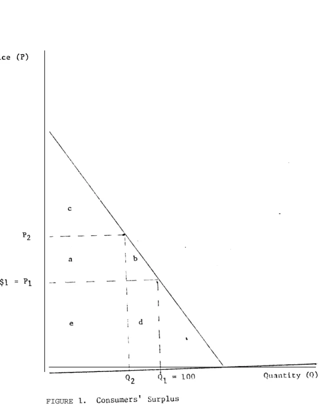
(3) 2.. an air of pseudo-objectivity to decisions on priorities but cannot serve as a reliable alternative to subjective judgment." tools offered up in this paprr complex,. 1. By no means are the. at least by the standards of my. profession; at most, they would ser-ve to improve subjective judgment at the planning stage but certainly not substitute for it.. Yet, as simple. as they are, they do become sometimes deficient in the face of the data available.. . These deficiencies-- constituting areas where really additional. research and information are needed--are highlighted in the last section of the paper along with major conclusions and implications of the analysis of the Colombian research programs.. Some Methodological Fundamentals. Consumer's Surplus The concept. of a consumer's surplus. was introduced by Dupuít over a. century ago, later popularized by Marshall, and ultimately extended by Hicks in the 1940's in ways which expanded and clarified its range of applicability.L. A simple, present-day definition of the concept can be made. by referente to Figure 1 and what is termed in the liternture a Hicksian ,$, : I compensated demand curve (HCDC) showing the maximum prices (P) a consumer would be prepared to pay for successive., additional units (Q) of a commodity.. If he were to pay &ch maximum prices al1 along until he had ob-. tained (say) 100 units, he would have made a total expenditure equal in. 1. 1. Arnon, Organisation and Administration ot Agricultura1 - - kesearch (London: Elsevier Publishing Company, Ltd., 19681, p. 123. 2. These early developments are reviewed by J. M. Currie, J. A. Murphy, and A. Schmitz, "The Concept of Economic Surplus and Its Use in Economic Analysis," Economic Journal, Vol. 81, No. 324 (December, 1971.1, pp. 741-800..

(4) Price. (PI. P2. $1 = Pl. FIGURE 1.. Consumers'. Surplus.

(5) 4. t value to the area under the demand curve and lcft of Ql in Figure @ (or the area a + b + c + d -t e).. If, on the other hand, he were to purchase. the 100 units on the market at a single avcrage price of $1.00 per unit, he would save a value equal to the area under the deasand $1.00 price line (area a f b + c). "consumer's surplus.'( consumers'. curve above the. It is this saving which is termed. For a collection of consumers or a "market," the. surplus is generally thc sum of individual surpluses of. consumers. Any factor which increased the market price of the good from Pl or $1.00 to (say) P2 would reduce consumer's surplus Figure 1.. by the area a + b in. This area can be shown to equal. wl~l. (1 - %Kn). (1). where K is (P2 - Pl>/Pl and n is the absolute value of the p‘ric;~ elasticity of demand.. 1. If K is associated with the change in average costs. of a commodity resulting from a new yield-improving technique generat:ed through research, then the above formula can provide a direct estimzte of the value to consumers of that research in a particular year, pro\ridt?d estimates are also available of PIQl and n. This rather simple and direct means of attributing a value ;.>r pladuct to a research activity has been criticizcd in the litertiturc >n :!:;a r:re~cndu. -. 1. The area a + 2b in Figure 1 equals KPlQl on this definitio*x, and the. area b equals. i~(Ql - Q,) (Pa - Pl) = $K2PlQln.. Therefore, cl-u.3 difIerence. betwcen these two quantities is equal to (1) above and the area 3 + b of Figure 1..

(6) 5.. that the value of n generally estimated is not exactly equal to thr value of the price elasticity of demand on the HCDC. 1. When the price of a. commodity falls to a consumer with a given money income, he is better off in terms of total utility or welfare because his real income rises. Since the consumcr's income is adjusted downwa-rd by the amount of this real income increase. following a fa11 in the price of the commodity in. the case of the HCDC but not in the case of an "ordinary" demand curve, the price elasticity of demand as ordinarily estimated can be expected to overstate the "true"' HCDC price elasticity.. If, for example, the de-. mand curve shown in Figure 1 were actually an ordinary demand curve, the HCDC would pass through the point (P2Q2) but evidente less slope. The implication would be that any estimate of the value of research to consumers based on equation (1) above would be biased downward. This bias has been overlooked in practice, First,. 2. primarily on two grounds.. it is argued that the actual value of the bias is small.. In Figure 1. the bias would equal in value only a piece of the triangle northeast of the demand curve formed by the points (P,, Q,), (P,, Q,), and (P,, Q,). The value of such a triangle is obviously small in relation ta the total area of consumer's surplus,. a + b.. Second, the magnitude of the bias is even. 1 For a recent example of this criticism, Ameritan Journal of Agricultura1 Economics, p. 177. 2. sec Wolfgang Bonig, "Comment," Vol. 56, No. 1 (February, 1974),. The actual direction of this bias, as well as the slope of t'he HCDC in relation to the ordinary demand curve, depends on the sign of the income elasticity of demand for the commodity. If the value of tlle income elasticity is negative, the bias referred to in the text would be in the opposite direction or upward..

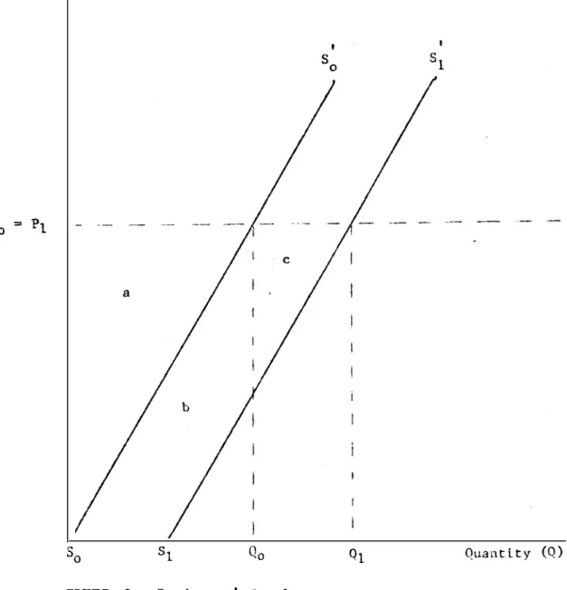
(7) smaller when the commodity in qurstion either has a small income elasticity of demand or represents a small proportion of total expcnditures on al1 commodities.. It is argued that the kinds of agricultura1 commodi-. ties for which research returns have been quantified using the consumer's surplus concept have, in fact, low income elasticities and represent a small proportion of total consumer expenditures.. 1.. Producer's Surplus The concept of producer's surplus surplus. is analagous to that of consumer's. and refers, in general, to a difference betwecn what is actually. received from the sale of a good and the minimum amount required to induce a seller to part with it.. Consequently, producer's surplus. has been equated. with an area--1ike a in Figure 2--between the prevailing price of a good and its supply curve since the latter has been traditionally defined as a locus of minimum prices at which quantities will be sold.. If the slpply curve. shifts to a position like that of S S' as a result of the adoption of a ll new production technique generated through agricultura1 research, then the benefit of that research to producers has been takeo equal to area b f c. Because there are sellers of input services like those of labor and capital,. 1. as well as sellers of final products,. al1 of whom could earn. A rather succinct defense of the use of the concept for purposes of estimating returns to agricultura1 research is contained in Ilarry W. Ayer and G. Edward Schuh, "Reply," Ameritan Journal of Agricultura1 Econorne, Vol. 56, No. 1 (February, E74), pp. 175 and 176..

(8) 7;. Pri.ce. (P). So. %. 0-0. FIGURE 2.. Producers'. Surplus. e. Ql. Quantity. (9).

(9) 8.. theoretically a "surplus," some confusion has nrisen over what producer's surplus a;J changes in it really measu.re. included, as the term implies, duction also included?. Is only the su~rplus of producers. or are surpluses earned by factors. of pro-. Alfred Plarshall, the author of the concept,. was. .. himself not clear on this point.'. It is of crucial practic%ìl significance. since any estimate of the product of agricultura1 research would be incomplete which included benefitc to consumers and producers but overlooked those accruing to factors of production. As ít turns specification.-of. out, what producer's surplus includes depends on the. the supply curve.. When variable inputs of production. are available to a competitive industry at prices which are independent of its leve1 of output, it is well-known that (a) the supply curve of the industry is the lateral sum of the marginal cost (or supply) curves of individual firms,. (b) the area under. Lhe industry's (firm's) supply- curve. represents the total costs of al1 variable inputs of production, and (c) the area above the industry's (firm's) supply curve bclow the prevailing price of the product is a return to al1 other inputs--namely, al1 fixed factors of production including inputs physically associated with the producer,. like his labor and "entrepreneurial capacity," as well as. other fixed inputs.. By definition these fixed inputs are specialized to. the industry or firm under consideration in the sense that thcy cannot produce anything elsewhere in the economy.. Therefore, on a bronder view,. there are no real costs associated with their employment; and any return to them would be an economic rent or surplus.. 'Currie,. Murphy, and Schmitz, op. a-t-., p.. Since producer's surplus. 754.. ..

(10) has been given the same definltion,. we may conclude,. tion posed earlier, that producer's surplus. in answer to the ques-. is a return to the producer,. as well as other fixed factors of production, and that there is a direct correspondence between the concept. at the leve1 of the firm and the indus-. try when prices of variable inputs are invariant with respect. to changes. in output. When some variable factors are not constant but increase. of production are supplied at prices which with the leve1 of an industry's output be-. cause their supply curves slope upwards, this simple interpretation of producer's surplus. disappears.. Assume that the sum of the marginal cost curves. of an índustry, SoSi in Figure 2, for example, shifts down to SIS; at the level.of. output Q, as a result of‘the adoption of a cost-saving,. technique generated through research.. improved. The value of costs saved, given our. definition of the supply curve, would be the area b. These savi.ngh, course,. would permit the industry to expand its output beyond Q,.. oE. However,. any output expansion achieved. through increased employment of variable factors of production would now tend to bid up their prices to the 5ndustry and make their costs exceed the area under the new industry sUm of marginal costs curve, SIS;, at anjr leve1 of output above Q, since the supply curves depicted in Figure 2 assume that unit costs of variable inputs are. constant.. Therefore, as output expands. marginal costs curve, SIS;,. in the industry,. the sum of. effectively begins to slip back to the posi-. tion of the initial supply curve, S S'. 0 0. Its final equilibrium position. would approximate that of the initial supply curve iE al1 variablt- inputs of production were subject to very inelastic supply curves. ?n that case the initial saving crcated by adoption of the new production tcchnique.

(11) 1. would have accrued mostly to the variable inputs of production as a surplus.. Area b of Figure 2 would then almost measure the change in sur-plus. derived by variable factors of production from the cost-snving improvement in production techniques resulting from research. ducers and other fixed factors. The surplus. of pro-. of production would be practically unchangcd. as would the leve1 of industry output (Qo). The final position of the supply curve of the industry would normally result in an output somewhere between Q, and Ql of Figure 2; that is, some variable inputs of production would be available at somewhat. higher prices. to the industry and, as output.expanded, the supply curve would shift . equlvalently from SlS; but not return to its initial level, S S'. The 0 0 area between this final positíon of the curve and the sum of marginal costs CUNE!. sls; up to the final leve1 of índustry output would then measure the. increase in expenditures by firms ín the industry on variable inpüts as a result of increases in their unit prices. Although such increased expenditures would represent vcry real increases in resources devoted to productíon by firms in the industry, they would not al1 be íncreases in real resources devoted to production from the point of view of the economy at large. since a part would accrue to. some of its nembers-- namely, to variable inputs or variable input suppliers-in the form of a surplus above their positively sloped supply curves and below their prevailing prices. That which is a surplus. should,. of course,. be accounted for as such and would be added to other estimated products returns to research.. or. To estimate such surpluscs cxactly, however, would. require data on the demand and supply curves Eor variable inputs employed by the industry.. Sínce they are not generally available, the most that. 0. ..

(12) 1.1 .. can be said usually is that the area between the final position of the sum of marginal costs supply curve of the industry up to the new leve1 of output and the sum of marginal costs curve which would have prevailcd had input prices been invariant with respect to output would represent an upperhound measure of the returns to variable inputs and their suppliers derived from the improved technique of production.. The area between the initial. and the final sum of marginal costs curve up to the product. price line. would then be a measure of the returns of the new technique captured. by. producers and other fixed factors of production. If the point of intersection of the vertical line through Q, with the supply curve SIS; were connected with the point of intersection 0% the .. new equílibrium leve1 of industry output with the price line, P 1. ' the resulting line would define a ncw supply curve which was adjusted for the kinds of considerations discussed above.. This "adjusted" industry supply. curve would have a smaller slope than the "unadjusted" sum of marginal costs curve of the industry or the relevant curve when prices of al1 variable factors. of production are invariant with respect to output.. To recapitulate:. Area b i- c in Figure 2 is an unambiguous measure of. an increase in the surplus the surplus. of ab1 fixed factors. of prOduCLiOA,. including. created by the producer from his self-employment, when vari-. able inputs of production are available to an industry at prices which do not change with output. industry. If variable input prices change with changes. in. output, then area b becomes a reasonable measure of increases. in. surpluses of variable inputs when their supply curves are very inelastic. If variable input supply curves are neither very elastic nor inelastic, IheA the area b + c is normally an upper hound estímate of the changes.

(13) 12.. in surpluses of fixed and variable factors. of production as it includes. some increnses in real resou'rcd costs to the economy. dustry supply curves have been identified:. Finally,. two in-. (1) the unadjusted sum of. marginal costs curve relevant when prices of al1 variable inputs are invariant with respect supply. to industry output and (2) an adjusted industry. curve, normally more steeply sloped and more inelastic, connect-. ing points on unadjusted supply curves after adjustments in them for input price changes.. Areas above and below this adjusted supply curve. are even more ambiguous than the arca b -t- c for reasons which are obvious on examination of Figure 2. Because of possible ambiguities ín the concept. of producer's surplus,. 1 shall refer to areas like b + c in Figure 2 as a "production surplus." (For similar reasons Mishan has argued that the term "producer's surplus" .. should give way to "economic rent. 'IL) To preserve euphony, I shali also refer to consumer's surplus. as the consumption surplus.. Combining Surpluses The definitions of consumption and production surpluses have been presented to this point with referente to a special. set of assumptions. about the slopes of the relevant demand and supply curves. for. In Figure 1,. example, which was used in defining what is now being called a con-. sumption surplus,. the demand curve oi the commodity in question was taken. . to be normally sloped, while its supply curve was taken to be perfectly elastic.. In Figure 2 the supply curve was normally sloped, while it was. the demand curve of the product which was assumed to be perfectly elastic.. 1 Vol.. E. J. Mishan, "What 1s Producer's Surplus?" Ameritan Keview, - - - - _ _ Economic ---__ 58, No. 5, Part 1 (December, 1968), pp. 1269-1283.. ‘.

(14) .. 13. These assumptions were nade for purposes. of exposition.. Ilaving 110~ mz;cìe. the essential definitions, however, the purpose of this section. is LO rc-. lax those assumptions and briefly titate the values for consumption and production surpluses which result when the price elasticity cjf demnd takes values of zero, a negative numbrr, and (negative) infinity, while the price elasticity of supply ranges in value from zero to a positive .:number and then to infinity. Although there are nine different possible combinations of these values of the two price elasticities, two have no meaning. a total of seven,. This leaves. two of which have already been discussed with referente. to the definitions of consumption and production surpluses and are shown as Cases 1 and II of Figure 3; the other five combinations of the price elasticities appear as Cases III through VII.. The hatched area of each. figure in Figure 3 represents the sum of consumption and production surpluses following adoption of a new production tcchnique generatcd search:. by re-. The large K is defined as (Po - Pl)/pl; the small k is (Q, - Qo)/Q 1 ;. So and Sl are, respectively, the original supply curve and the one which prevails after adoption of a new production technique; n is the absolute value of the price elasticity of demand; and e is the corresponding value for the supplT1 curve. It can be seen that al1 cases are special. cases of Case VI.. From the. first expression for the shnded area of Case VI, Case 1 can be derived by letting e go to infinity; Cases V and VII result from setting n equal to zero.. From the second expression for the shaded area of Case VI, Cases. II and IV can be obtained by letting n tend to infinity; by letting go to zero, Case III is derived.. e. That there are two expressions for the.

(15) Case I KPIQl (1 - % Kn). Case III. Case IV. Case V. kPIQl. K'lQ,. P. E \ Case VI. Case VI-C. -Q.

(16) Case VI shaded area simply refl.ects the approximate nature uf al1 formulas.* Refeyence to thc expressions given to the shaded areas of Figure 3 produces two inferences:. (1) Al1 formulas for the combined surpluses derived. from the adoption of a new production technique involve only a few paramsters-PlQl and a constant,. which includes. k or K, n, and e; and (2) total surplus. would be expected to be greatest when estimated. under Case III assumptions. and least under assumptions of Case 1, other things equal.. Additional Issues Before turning to applications of this methodology to plant-breeding research in Colombia, a few concluding comments about what has been said thus far are in order.. 1.. Since the areas between the supply curves do not provide always unambiguous measures of production surpluses--and,furthermore,. those surpluses cannot be disaggregated by. source, e.g., "producers" and '"inputs'8--consideration should be given in future work to estimating production surpluses directly from the demand and supply curves of. 1. Nicolas Ardito Barletta, "Costs and Social Benefits of Agricultura1 Research in Mexico" (unpublished Ph.D. dissertation, University of Chicago, 1971),Appendix C, has provided the following formula for the Case 6 surplus:. Willis Peterson, "Returns to Poultry Research in the U. S.," Journal of Farm Economics, Vol. 49, No. 3 (August, 1967), pp. 656-669, hGg=ced:. kQ,P, + k. 2 plQl. yy-- -.

(17) 16. production inputs.. In Latin America where the distribution. of surpluses between factors. of production assumeri fre-. quently as much importance as the aggregatc value of the surpluses themselves, this suggestion may be especially relevant. 2.. If there exists ínput unemployment in agriculture and it i.G reduced as a result of the adoptíon of yield-improvíng new techniques generated through research, earnings of the otherwise unemployed ínputs should be added ín as a productíon surplus (benefít) of research, not as an additional resource cost.. 3.. 1. Combined production and consumption surpluses are commonly estimated and presented first as an aggregate and then disaggregated or divided between "gproducers" and “consumers'c ín an attempt to show who has gained most from agricultura1 research. 2. This is not done ín the sectíons which follow.. The means by whích the disaggregation is performed should be readíly apparent in the review of the methodology which has been presented to thís poínt. 4.. A closed economy has been assumed up until now.. If the. colmnodity affected by agricultura1 research is, howevcr,. 1. For an interestíng applícation along these lines, see A. Schmitz and D. Seckler, "Mechanized Agrículture and Social Welfare: The Case of the Tomato Harvester," Amerícan Journal of Agricultura1 Economics, Vol. 52, * No. 4 (November, 1970), pp. 569-578,. 3. iost recently, this has been done by Harry W, Ayer and G. Edwrtrd Schuh, "Social Rates of Return and Other Aspects of Agricultura1 Research: The Case of Cotton Research in S& Paulo, Rrazil," Ameritan Journnl of Agri__I-_~ cultural Economics, Vol. 54, No. 4 (November, 1972), pp. 557-569..

(18) 17.. traded in foreign markets, some nominal modifications in the analysis need to be made. Figure 4 assumes. that a commodity subject to a shift. in supply of Ql - Q, is imported at a world price, Pl, which is unaffected by the leve1 of imports of the country in. question.. tion surplus;. The supply shift does not change the consumpits only effect is on the side of production.. The shaded area between the two supply curves up to Q, would represent a surplus. to society since it involves a saving. in the costs of producing Q . The remaining triangular 0 shaded area would also be included as a benefit, although it is derived from a different source, corresponding as it does to a saving resulting from producing more of the commodity locally.. Figure 5 assumes. that the commodity in. question is exported, rather than imported, at a price Pl, likewise invariant with respect sold by the country in question.. to the leve1 of exports If supply shifts from. Q, to Ql, the only "benefit" would be a production surplus equal to the shaded area of the figure. 5.. There is no easy, straightforward, or "most recommended" way of measuring the shift parameter curve attributable to research. for. 1. 1. k of the supply. It has been estimated,. example, on the basis of essentíally an educated guess. The only fully "open economy" evaluation which has come to my attention, aside from the "partially open" Ayer and Schuh study cited above, is the one done by Y. Hayami and M. Akino, "Organization and Productivity of Agricultura1 Research Systems in Japan," to be presented to ä Confcrence on Resource Allocation and Productivity in Intcrnational Agricultura1 Research, January 26-29, 1975..

(19) Price (P) I. Ql FIGURE 4.. Quantity. Production Surplus. (Q). with Irnports. Price (P) I Pl. Qo FIGURE 5.. Production. Q, Surplus. Quantity with. Exports. (Q) ".

(20) 19. by Griliches,' as a shift ín the long-run supply curve by Peterson,. 2. on the basis of estimates of farm-leve1 produc-. tion functions by Ardito, 3 and from experimental yield data by Ayer and Schuh. 4. In the research reported in the. next sections of this paper, yield differences estimated from on-farm trials run by the research program itself are'incorporated into estimates of the shift parameter. The tact taken in al1 cases, including those reported here, has been determined probably more by the availability of data than by any more superior arguments of theory and reason!. Rice5. Colombia's rice research program is of relatively recent been initiated in 1957 by the predecessor agency of ICA. ment coincided. origin, having Its establish-. with a Sharp rise in rice imports occasioned by an outbreak. 1. Zvi Griliches, "Research Costs and Social Returns: Ilybrid Corn and Related Innovations," Journal of Political Econ-, Vol. 66, No. 5 (October, 1958), pp. 419-432. 2. Peterson, op.. cit.. 3Ardito, op. cit. 4Ayer and Schuh, op. cit.. 5 This section draws heavily on the work by Jorge Ardila, "f~wztubi~icihd Socia2 de Zas Inversiones ex Investigueion de Arroz en CoZombZatt (unpublished M. S. thesis, ICA/National University Graduate School, Bogota,. 1973)..

(21) 20. of the hoja blanca distase,. 1. a virus of Latin America--with sbwptoms. the stripe dissase of Japan--which first caused substantial losses Venezuela in 1956 and in Colombia itself in 1956 and 1957.* ingle,. like in. Corrcspond-. the initial objectives of the research program includcd. varietal. selection and breeding for higher yields and resistance to the hoja bkznca virus. Rice varieties with resistance characteristics were collected throughout Colombia as a first step; in addition, 2,200. varieties. were. selected. and imported from the U. S. Department of Agriculture"s World Collection of Rice in Beltsville, Maryland.. By 1959, about 400 of these varieties. had shown promising resistance to thc virus.. 3. Because they were japonica. varieties in the main, previously not consumed in Colombia, the research program adopted an objective of breeding the virus-resistant characteristics of japonica into the local long-grain varieties. 4. It was esèimated. Iv. ntil 1957 Colombia's imports of rice were running around 2,000 metric tons annually. The 1956 crep was down about 10 percent from 1955 (from 324,000 tons in 1955 to 300,000 tons in 1956), and the 1957 crep was up less than 8 percent from 1955, in part because of a fa11 in yields. In 1957 Colombia then imported 10,200 tons of rice. In 1958 and 1959 imports Refer, for example, to relevant issues of returned to "normal" levels. the FAO Rice Report for these and related data.. 2 S. H. Ou, Rice Diseases (England:. Comxonwealth Mycological InstiApparently the attack was least scvere where the tute, 19721, pp. 28-33. Colombian red rice was grown; see Philippe Leurquin, "'Rice in Colombia: A Case Study ín Agricultura1 Development, " Food Research Institute Studies, Vol. VI, No. 2 (1967), p. 231.. 3The means by which the disease was transmitted were not identified with the insect, Sugotodes, until 1958. -> 4 Chemical control of the virus provcd somewhat effective--but very expensive-- among partially resistant varieties; see G. E. Galvez, ‘í!o;ia Blanca Disease of Rice," The Virus D-iseases of the Rice Plant (Baltimore: Johns Hopkins Press, 1968), pp. 35-49..

(22) 21.. As an in-. that this objective might be satisfied in four to five years.. terím medsure, the one superior-yielding U. S. variety which had shown some virus resistance, Gulfrose, was multiplied and released. in 1961.. The first ímproved variety, Napal, to be produced by the Colombian research program was actually released in 1963 or just four years later. Napa1 had the long-grain characteristics of Bluebonnet 50, the most preferred nontraditional varíety, but was resistant to hoja b.lan.ca.. IL. Un-. fortunately, Napa1 was selected out in 1965 for a heavy attack of Bruzone (rice blast disease) and dísappeared thereafter from commercial production. In the same year, Tapuripa, earlier imported from Surinam, was multiplied and distributed to farmers as an alternativa to Bluebonnet 50 and Gulfrose.. It was long grained and flinty with some resistance to blast dis-. ease and hoja bZaxca. In 1966 the Colombian rice research program added an objectíve whích reflected leads of the International Rice Research Institute (IRRI): to develop dwarf varietíes with a high grain-to-straw ratio and resistance to. lodging.. About 3,000 additional varieties were imported from IRRI,. and an order went out that only those varieties already in the Colombian collection should be retained which out-yielded Bluebonnet 50 by 100 percent. A year later ín 1967, ICA's program joined forces with the rice program of the International Center for Tropical Agriculture (CIAT). Personnel, facílities, budgetary resources, and objectives were shared under informal agreements between the two institutíons.. These had the effcct of reinforc-. ing the ties of the Colombian program with IRRI as the head of CIAT's rice work had served. 1. on IRRI's staff.. Bluebonnet 50 was Eirst imported to Colombia in 1954. The history of its introduction and rapid adoption is discussed by Lcurquin, op. cit., PP- 250 and 251..

(23) In 1968,CIAT and ICA introduced IR-8.. Its adoption advanced well. even though the medium-type chalky gra-in sold generally at a 30 percent discount, and susceptibility to blast disease was evidenced. prove resistant to hoja blanca.. IR-8 did. Following strong commercial trade in-. terest, CIAT and ICA also introduced IR-22 in 1970 and recommended it to farmers in irrigated tropical areas. Between 1966 and 1970,ICA released independently two additional rice varieties, ICA- and ICA-10.. These never assumed any commercial importance,. however, because their yields were inferior to the IRRI varieties--whi.le being superior and/or more certain than either Gulfrose or Napal--and their grain quality was less desirable than Tapuripa. In 1971,CIAT and ICA released the CI.CA-4. '. variety.. It was more disease. resistant and had greater water and air temperature adaptabilíty, good grain appearance and cooking qualities, and slightly superior yields. Simultaneously, CICA-4 appeared in Ecuador as IN-IAP-6,. in the Dominican. Republic as Advance 72, and in Peru under the name of Nylamp. Yields recorded in commercial field trials of the seven major rice varieties released by the Colombian and joint CIAT-ICA programs after 1957 are shown in Table 1, tc/gether with data obtained from the same source on yields of the check variety, Bluebonnet 50.. The 665 individual trials. which are the basis for these yield statistics include al1 that are available for the 15-year. period, 1957-1972.. commercial trials or pruebas regionaks. It should be mentioned that ICA's are conducted on parcels of com-. mercial farms which agree to collaborate with Che Institute's programs. Farmers run the trials, but materials and instructions are provided by KA.. *.

(24) 23.. .. CTJ P 0.

(25) 24. The three rice varieties released. prior to 1966 show average yields. in these daca of 4.1 metric tons per hectare representing a yield advantage over Bluebonnet 50 of about 33 percent.. Varieties introduced after 1966,. including ICA-10, just double that yield advantage bringing it to 65 percent above Bluebonnet 50. In view of these yield data, it is interesting to note in Table 2 that the area planted to improved rice varieties did not become a significant proportion of al1 riceland until the second, or post-1966, stage of the research program.. Data in the table on the percentage of acreage. sown to a given variety were estimated ín the following way.. First,. available information on sales of certified seeds by variety were converted to hectare equivalents by dividing by estimates of seeding rates provided by ICA's Director of its National Rice Program.. Second, it was. assumed that the proportion of al1 acLeage planted to certified seeds OE any variety was equal to the proportion planted to later generation seeds of that variety produced by farmers outside the seed multiplication and certification program.. Thus,. the percentage of acreage sowu to a variety. which is shown in Table 2 equals two times the percentage sown with certified. seeds.. This estimating procedure has the effect of equating the. percentage chcnge in area planted to an improved variety with the percentage change in sales of its certified seeds.. Since the latter rate would. be expected to taper off before the rate of growth in area planted, the net effect of the procedure is to underestimate the true leve& of adoption of improved rice varieties.. This is doubly true in the case of Lhe. estimated percentage of riceland planted in al1 improved riceiarieties as data on Gulfrose seed sales could not be located..

(26) TULE 2 Colombia:. Yenr. Land Area Planted to Six Improved Varieties of Rice as a Percentage of the Total Area Planted in Rice 1964-1973. Variety Napa1 1 Tapuripa 1 ICA- 1 IR-8 percent. I. IR-22. 1. CICA-4. al. Al1 improved varieties 2.5 2.1. 0.1. 0.1. 3.2. 0.1. 21.2. 0.6. 0.3. 22.1. 1969. 18.0. 0.5. 3.7. 22.2. 1970. 12.4. 0.2. 18.2. 30.8.. --L--. 3.3. 26.1. 3.1. 5.0. 11.1. 1972. 18.9. 10.1. 18.3. 47.3. 1973. 20.1. 24.3. 12.6. 57.0. 1971. -a/ Blanks indicate. 6.9. less than 0.1 percent.. Sourccs: Social de Zas Inversiones en Invcs~i.garion de Jorge krdila, “RcntabiZidad .fm’O~ en CoZoc?bia" (unpublished M. S. thesis, ICA/National Univcrsity Graduate Sch~ol, ZoCota, 1973), Table ll for the years 1964-1971; also, after 1971, IC.4, Dirl?ctor of thc National Rice Progran..

(27) 26.. In order to estimate the shift parameter of each new variety--its yield. advant?ge over Rluebonnet SO;-production functions. pmebas m@onaZcs. data using standard. final round of estimation, 20. lrast-squares procedures.. In t-he. reported yields were taken as a function of. variables: size of the trial plot, seeding. ables,. were fit to the. rate, 7 seed variety vari-. 2 variables to distinguish different time perio&,. 4 variables re-. loting to irrigation and its interactions with seed variety,. and 5 vari-. <Ibles to differentiate locations and their interactions with variety. Only the first two of these variables entered Other. continuous variables (relating. as continuous. arguments.. particularly to "cultural practices"). were either discarded or respecified in noncontinuous form in the final results presented in Table 3. Since the estimated. coefficients on the variety variables are to be. interpreted as their "yieldWdisadvante~eg" with CICA-4,. it is evident. in kilos per hectare compared. that Colombian rice research has produced. through time continuous and substantial improvements in yields.. Again,. the superiority of the post-1966 releases is evidenced. The large and significant. coefficient on the variable adjusting for. some of the 48 locations used for the pmebas rq~oxutes indicates yields of al1 varieties are increased that this effect ties,. 1. is somewhat. larger. that. by about 1.2 tons in those areas and. for the Napah,. Gulfrose,. and IR-8 varie-. the location-variety intcraction variables for which are positive.'. The location variable assumed a value of one when a trial fe11 into areas which could be classified as tropical dry forest, subtropical humid Thcse classificaforest, or very dry tropical forest and zero otherwise. tions were suggested by the Director of ICA's National Rice Progrnm..

(28) 27.. TABLE.3 Production Function Estimates for Rice Colombia: Based on Commercial Trial Data, 1957-1972. Estimated coefficient. Independent variable. Estimated t statistics. 1.. Size of trial plot. 0.15. -2.30. 2.. Seeding rate. 2.46. 1.58. 3.. Bluebonnet 50. -1,609.66. -3.45. 4.. Gulfrose. -1,486.56. -1.31. 5.. Napa1. -1,742.79. -1.83. 6.. Tapuripa. -. 884.31. -1.80. 7.. ICA-. -. 536.93. -1.13. 8.. IR-8. -. 798.97. -1.54. 9.. IR-22. -. 589.97. -0.72. 10.. Irrigation. 1,220.20. 5.84. ll.. Irrigation * IR-8 interaction. lj78.09. 3.21. 12.. Irrigation * IR-22 interaction. 700.44. 0.89. 13.. Irrigation * CICA-4 interaction. 1,061.87. 2.11. 14.. Location. 1,185.26. 7.12. 15.. Location * Gulfrose interaction. 991.98. 0.94. 16.. Location * Napa1 interaction. 940.33. 1.06. 17.. Location * IR-8 interaction. 428.22. 1.24. 18.. Location * CICA-4 interaction. -1,340.16. -1.14. 19.. Time 1. 1,228.03. 6.74. 20.. Time II. -. Intercspt. 509.78 2,028.30. R2 = 0.67. -2.20 3.64 n = 665. --. Socia2 de Zas Immwionzs t??z Invcr;tigacxhn Source: Jorge Ardila, 'tRentabiZidcxd de Arroz en Colomb,ia" (unpublished M. S. thesis, ICA/National Un'ivarsity Graduate School, Bogota, 1973), Table 13..

(29) 28.. The Eact that the corresponding interaction term is negative and about . equal to 1.2 tons in the case of CIU-4 leads to a conclusion thnt it is the only variety which is less location specific. Results suggest, however, that yields of CICA-4, as well as of IR-8 and IR-22, are very positively influenced by irrigation.. thos2 The. co-. efficient on the irrigation variable indicates that ylelds of al1 varieties are increased by about 1.2 tons with average irrigation practices.. Roughly. another ton is added on top of this when irrigation is applied to IR-8, IR-22, or CICA-4 as indicated by the coefficients on the variables of interaction of those varieties with irrigation. This evidente from the production functions, coupled with data which show that dryland rice yields increased 7 percent during the 1961-1972 period while those of irrigated rice increased 133 percent, 1 leads to an inference that the newer varieties have benefitted mai.nl:r the irrigated rice areas. zI -The other side of the same coin, of course,. is that adoption of improved. varieties was assisted by the existence of irrigated cropland. Most of ICA's research has been focused on the irrigated rice arzas. Its largest programs have been located at the Palmira and Espin%l experiment, stations.. Wbile about 75 perzent of al1 riceland is irrigated today. (1974) in Colombia, almost 100 percent has been traditionally irrigated within the areas served. by Palmira and Espinal. 3. 1. FEIDEARROZ, In.forme de Gerencia nZ X.TIT Colombia, 1971, p. 32.. Underscoring this po.int. Conyreso. Nu,oionuZ, Bogota,. 2. In 1948 Raul Varela Martinez, Industria y commcio de-A:PPo:< - en C~~h~%icx (Bogota: Miwkterlio de Agricultura y GcLnader(zi, 19491, p. 15, cstimnted that 18 percent of al1 riceland was irrigated and 16 percent wa:; partly irrigated. By 1974, it is estimated that the perccnt of ricelaad irrigated had increased to about 75 percent. 3. See, for example, Leurquin, op. cit.,. Tables 5 and 11..

(30) 29.. is the fact that 84 percent of the ~I>^LW~~CI irrigation.. ~~~iorwZas were performed. with. Also, among the 48 locntions uscd for experimentation, upland. rice trials were the only type performed in 14 locations while 30 were used only for trials with irrigation. have been induced. This emphasis on the irrigated are-as may. by expectations of th e sort of variety-irrigation inter-. actions found in the regression results.. More plausible is the common-. sensical explanation that ICA's creditability would have been seriously questioned had it not produced. vari.eties which yíelded well in the irri-. gated areas of Colombia since the controlling interests of the rice growers and commercial trade are found there. 1 Regression results were used to produce two estimates of the overa11 shift parameter-- the percentage change in rice supply attributable to the yield advantage of al1 the improved varieties over Bluebonnet 50. taken to include only "varietal. One was. effects" on yields and estimated as a. weighted sum--divided by average commercial yields--of the regression coefficient of each improved variety minus the coefficient corrcsponding to Bluebonnet 50, with weights equalling the percentage of al1 riceland planted which was sown in each variety.. 2. A second estimate of the shift parameter. derived from the regression results was taken to include other varietyspecific interaction effects in addition to the direct varietal effects of the first estimate.. This estimate is shown in coïumn 3 of Table 4,. It was reported that half of the value oE all. dues lIbid., p. 259. collected by the National Federation of Rice Growers has come from Tolimn. 2. The exception to this procedure IJaS taken in estimating CICA-4's yield advantage since, given the specification uf the regreusion, the yield advantage of CICA-4 rquals simply the negative value of the coefficient on Bluebonnet 50..

(31) 30.. TABLE 4 Colombia: Altrrnative Values of the Supply Shift Parameter for Rice Attributable to Improved Varieties, 1964-1971. 1. Estimate Varietal plus interaction effects 3. Year. Simple 1. Varietal effects 2 nercent. 1964. 1.05. -0.17. 2.18. 1965. 1.01. -0.15. 1.90. 1966. 0.13. 0.05. 0.17. 1967. - 0.17. 0.38. l.ú5. 1968. 10.99. 5.64. 13.37. 1969. 12.81. 4.91. 14.85. 1970. 14.89. 2.85. 21.48. 1971. 15.96. 8.16. 32.12. -. -. - - Based on Jorge Ardila, "UentubiZidad Social. de ZGS en Im~stiyacion ds Arroz en CoZombLa" (unpublished M. S. thesis, ICA/National University Ciradclate School, Bogota, 1973), Tables 5, ll, 12, 13, 17, and 20.. Source:. Imersiones.

(32) 31. along with the "direct varietal effects". estimate. presented in column 2,. 1. and a "simple" estimate of the yield advantage of the improvecl varieties. (shown in column 1 of the table) which is based on the averagc? annual yield data for each variety obtained in the pruebas xlcgfonales and already presented in Table 1. The fact that the simple estimates of the shift parameter exceed the zstimates which include just uarietal effects from the regression is consistent with the finding that only the improved varieties of rice interacted with other variables of the production function.. Since those inter-. actions were on balance positive and are included ín the simple estimate but not ín the varietal-effects estimate, the simple estímate overstates the shift parameter by as much as 12 percentage points.. Simílarly, the. estimates based on the regression whích include varíetal effects plus the variety interactíons exceed the varíetal-effects estimates because-variety interactíons were posítive valued, yet less widespread than available data indicated.. 2. The simple and varietal-effects estimates were combined. with assumed. values of the price elasticities of supply and demand to provide upper and lower bound estimates of gross social benefits of the new seed varieties. 1. The estimates in these two columns evidente lower values for the shift parameters than the source (Ardila, OP. cit., Tables 17 and 20) by rt‘a:;on principally of the omission here of adjustments for "time." Ardil.a orit;i.nally dddcd to the yield differentials estimated from the.production functions appropriate values of the coefficients on the time variables in each year. Since those coefficients are on net strongly positive for the 1964-1971 period, the effect was to increase estimated values of the shift parameters. 2. The only data availnble related to the amount oE riceland irrigated in each location..

(33) 32. . for the period 1964-1971.'. Values considered fo-r the price elassicities. of supply wele zero, 0.2347, and infinity, the intermediate value being derived from the only supply study available for Colombian rice;:!. values. considered for the price elasticity of demand were -0.5, -1.372, and -2.0, the intermediate value again having been estimated ín another study.. 3. Maximum gross benefits resulted from using the simple estimatcs of the shift parameter and pricc elasticities of demand and supply, respectively, of -0.5 and zero; minimum benefits corresponded to price elasticities of. demand and supply of -2.0 and infinity and the varietal-effects estimate of the supply shift parameter.. Both these estimates are shown in Table 5. for the 1964-1971 period. Costs of the research program for the same period, also shown in Table 5, include direct costs, indirect. costs, and complementary costs, definitions. given these terms being those earlier Llsed by Ardito. 4 rice progran were available only after 1964.. Direct costs of the. For this reason available. cost. data were regressed on the number of employees assigned to the rice progrnm and ICA's total expenses for al1 research programs;. the resulting regression. coefficients and available data on the two independent variables of the. 1. Calculnti>ns based on the varietal effects plus interaction etfects shift pararneters are not included here but can be inspected in Ardila, OP. cit., Table 27.. 3&i.J. 4. Table 4.. Ardito, op. cit..

(34) 33.. TXBLE 5 Colombia: Estimated Renefits and Costs of the Rice Research Progrnm, 1957-1980. Year. Estimatej Max-imum 1 1,C. 1957 1958 1959 1960 1961 1962 1963 1964 1965 1966. 51. /. 193 235. 3,733. 599. 286 429 441 252 445. 4,750 553 827 61,659 60,872. 699 213 1,849 26,887 19,673. 538 519 867 937 2,074. 1.1. > 24 3 43,488 43,5L7. 2,779 4,165 4,202u. 69,444 107,470 107,543. l i. I. a/ Blanks indicate no benzfits. b/ -. This figure was assumed for 1972 nnd figures Für subsequent years were estirnated by assuming 4,202 gres 10 percent clnnualby.. Yources: Cols. 1 and 2:. Based on preced. ng. tnhles..

(35) 34.. regression were then used to estimate the direct cost data for the missing years, 1957-1965.. Complementary costs associated with the new program--. those it incurred with other collaborating programs--were estimated for this study by the Director of the National Rice Program. associated with the entomology, plant physiology, and extension programs.. Indirect. Included were costs. plant pathology, soils,. costs were taken to include staff train-. ing costs,' opportunity costs of t-he services. of fixed capital and land,. management costs, and the costs of "international cooperation" including a prorated share of personnel costs of Rockefeller Foundation staff stationed in Colombia from 1958 through 1968 and, most importantly, the total costs of the CIAT rice program from 1969 to 1972 cstimated by the head of that. program.. This latter item was the major cost.. The simple sum of. total costs for the 1957-1971 period equalled 14.2 million 1958 pesos, -. .. and the costs of international cooperation were calculated nt 5.0 -million or 35 percent uf the totrtl.. 2. Recognizing that the current stoclc of new llarieties wi.11 continue. to. produce into the future, costs and benefits of the Colombian rice program were projectcd forward for nine year:; to 19817 usina assumptions,. when. necessnry, which would bias dotynwards the estimate of interna1 rates of rcturn. of the. It was assumed on tht- cost side, for cxample, COO~JeratiVe. that tile real value. CIAT-ICA rice progrnm woulcl increase at a ratë of zbout. 1. .. Cne staff menb~r of the rice program WILC; trilíned thrc>ug:!l ti,c 1'il.D. I c o s t s of trLl i r! iris pc?i-and four othcrs mere trairltid through tht‘. Ft. S. sonnel of the National F'cderation oL Rice Crower:.; at the Natíon:ll Liniversity/ICA Graduate School were also included. 2. Costs of international cooperation are still probably undcrstated since benefits derived from the IRRI "capital stock" irave not been charged to the Colombian program..

(36) 35.. 10 percent per year, primarily on the grounds. that programs which are. relatively new and reputedly successfu.1 tend to grow!. 1. On the side of. the projection of gross benefits, it was assumed that thc value of production during the 1972-1980 períod wbll average %81,000,000 pesos, a sum which equals the value of the rnther good 1971 crep (in 1958 pesos); that the rate of adoption of the new rice varieties after 1973 will stabilize at the estimated 1973 leve1 of 57.0 percent;2 that the percent of riceland planted to IR-8 will trend downward linearly to zero by 1980; that the percentages of al1 riceland sown to IR-22 and CEA-4 w-I.11 be equal after 1973; and that the increase. in the shift parameter these as-. sumptions would imply will about equal increases in commercial yields over the period 1971-1980.3 The resulting interna1 rate of return corresponding to the stream of maximum gross benefits was found to be 82.3 percent; the rate estimated. 1. Since this ;~ssumption was made, KA':; budget has brrn sevrrely cut and CIhT's rice program Llas been phased dovn. Non?theless, we hold to the initinl assumption in ordcr not ti, ovcrstate thr final c:;timatc of tire interna1 rnte 02 return. 2. This is a more modtiratc assumpti.on than that used by ArrliLa, "2. c-i:., Table 35, who assumdd thtt the percentage of area sown in irqrov& ric;: Th> data of LLIL would fa11 bztween 72 perccnt and 84 percent by 19:ìO. LJ. s. Ddpartment of ‘IgricuZture, Economic liesearclh Servicc, Dk:v~~~Lopm~nt ~-_-_-.-___che Les:;-sud Szead oE Li-igh-Yie Lding Varíetit3L; of Kheat aritl Kicc- in __-.-.-_ .~--.___. _---._-. --.--____I------.Developed Nation~, EAER No. 95, 1974, Table 38, í.ndicatirtg that adoption Irates in the Philípp-ines, Malaysia, and India are topping out at: ratel; well undcr 60 percent, plus the anaI.ysis by Robert Evenson, "Thc 'Creen Kevolution' in Kecrnt Dcv&oprnznt Experience," Ameritan .Joi~rn:iL----of -..1__ J:;r i___.__ __-cultural Fkonomics, Val.. 56, No. 2 (Gy, 1974), pp. 387-394, su:;gcst that the use of ~mprovèd variet ies may n~'vcr ~-cacl~ 70 per<ent in Coli>inbi;i :tr:cl that an as:;umptiotl of 57 pc'rccnt .is !ilOTè corl:icrvLttivt? anil ~~~Oll~~l.~ le. 3. The irlcreascs in yizlds would be Ll+ and í.1 p~:rcent 1 respectively, for the m;lximum and mínimum values 01 tlw sllí.ft Ljar;lmeters..

(37) 36.. on the bas-!s. of the mínimum gross benefits stream was 58.0 pcrcent. 1. 130th. are well ín excess of the social opportunity cost of capital of about 10 percent which has been calculated by Ilarbergcr for Colombia.. Costs in each year. could have been 6.1 times larger than estimated, and the maximum gross benefits would still have provided a 10 percent retur&i research;. oA1 investments in. a 10 percent return would have been obtained on the stream of. minimum gross benefits had costs been increased in each year by two times.. cotton3. Cotton has turned in a striking growth performance in Colombia. Since the mid-1930's, yields have about quadrupled--in fact, their pattern of change has been broadly similar to that of the United States. Currently, Colombian cotton yields are comparable to U. S. yriclds and.

(38) 37.. TABLE 6. Comparative Cotton Yield Stacistics 1934-3511938-39 to 1973-74 -..--__. South 1. UnLtcd Colc )mbia 7 All. crops 1. Year. index al. 1934-35 to 1938-39. I 2. Ameríca. I ll----ounds per acrl. 4. 133. 212. 181. ! 1 l. ;. 1947-48. 100. 152. 267. 163. 1950-51. 115. 167. 2 6 9. 175. 1951-52. 102. 1so. 269. 203. 1952-53. 109. 227. 280. 197. i !. 1953-54. 119. 317. ' 324. 212. l. 143. 319. 409. 1.78. 1959-60. 152. 377. 462. 207. 1962-61. .L 7 íi. 398. 457. 331. 1965-66. 1.5 8. 3 52. 526. 244. f96ó-67. 164. 4 I0. 4hO. 232. 1967-68. 17 6. 5.L6. 447. ?67. 1970-71. 463. 437. 1973-74h'. 470. 519. 1956-57. I. --.I I_--__. 1___-___-. !.

(39) 38.. 1950-1960 period among those. 24 countrics. 97. percent of al1 cotton in 1960.1 creased. of the world which produced. Production. after. the. mid-1930's in-. at least 15 times or from about 30,000 hales in 1937-38 to over. . 500,000 bales in the eaarly Yields atid. 1970's.2. production advanced. widely separated periods. of time:. doubled in the first period. production. evidenced. most rapidly in two different but not. a much. 1951-1954. Although larger. and. 1957-1959.. Yields. about. khey did increase in the second,. inrrease. of. in both periods appear to have been the direct. 167. percent,. Dcvelopments. result of changes. in gov.. ernment policies. The first period of rapid. developmrnt. Colombian Ministry of Agriculture. in 1948 and nsw. emphasizing the need tu substitute .. production.. cotton--which. resulted. between 1948 and 1951e3 the prospect. imports. policy pronouncements. of food arrd fibers with. local. In the case of cotton, rhis involved some protection;-notably. a requirement that the textále tional. followed the reopening of the. of consuming. íutiustry consuae scated allotments in nn 82 percent increase. When the local 6kxtIl.t:. irdustry. larger qualltbties ajf nation~l. of na-. in the farm price W~L; fziccd ~OCCG~~,. wi.th. ir promrJted.

(40) 39. the establíshment ín 1948 of the Cotton Development Institute (IFA) for purposes of improving the quality and uniformity of local cotton through research and the control of ginning. 1 stitute with its own budget, also tension,. seed. distribution,. The second surge in paralleled changes. and. IFA, eventually a governínent in-. assumed responsibilies for cotton excredit.. production, occurring at the end of the 195O's,. in exchange policies.. Colombia was 2.5 pesos per U. S. dollar. The official exchange rate. in. from 1951 through May, 1957. Thz. free rate was 3.0 to 3.5 pesos through 1954 and then edged up to 6.9 pesos by. mid-1957.. Through. the. On June 18, 1957, the official rate 1951-1957. was increased to 7.6 pesos.. period, the Colombian textile. industry was permitted. to import raw cotton and capital items at the official exchange rate.. As. a result, imports steadily built up to a leve1 of 77,000 bales in 1957; production stood at 95,000 bales in that same. year.. reforms, production jumped to 220,000 bales and, in bales.. In 1958, following 1959, reached 256,000. Imports fe11 to 36,000 bales in 1958 and to slightly less than. 2,000 bales in 1959, at which time Colombia also able surplus. of cotton in severa1 decades.. showed its first export-. During the early 196O's,. ex-. ports averaged about 100,000 bales and by 1968 had reached a leve1 of almost. 300,000. bales.. As producers. of cotton attained national prominente. satisfying domestic tional Federation of In 1968, IFA. 1 Leurquin,. and power for. consumption and exporting a growing surplus, Cotton Growers (FNA) began to absorb IF.l's. the Nafunctions.. was dissolved completely; and its research and extension. "Cotton Growing in Colombia . . .," pp. 158 and lS9..

(41) 40. activities. were passed on to the ICA.. sorbed by the Ministry -_. suspended. ín 1948.. when attention. for. Cauca Valle). in 1928 but was later. there turned to the prospect:; for sugarcane. mission. from Puerto Rico.. later (1934) in Armero,. U. S. Uplands. responsibilities. On the advice of an English mission,. was begun in the. search by a visiting lished. was meager when it assumed. cotton research. some cotton research. were ab-. of Agriculture.. IFA's inheritance organized. Others of its activities. State of Tolíma,. and some Peruvian. varieties.. Some research to introduce. Most progress,. re-. was estaband test. however,. until 1948 had been made in improving. the perennial. tion on the outskírts. on the north coast is reported. of Barranquilla. tree cotton.. up A stato. have obtained. yields of 350-400 kilos per hectare or at least twice the then prevailing average yield. 1 Nonetheless, one of the first things IEA ?. did was to close that station sidered. inferior. with diseases. to imported. which threatened. From the beginning, introduction, ties.. testing,. No attempt. as the quality. of the tree cotton was con-. cotton and tree cotton had become i.nfested the introduction. the Institute's. sole research. and multiplication. of improved. was made to produce a national. that effort appears. to have languished. of annual varieties. objective. was the. U. S. cotton varie-. variety. until 1961, anll ‘* until IFA's research was absorbed. by ICA in 1968. ICA stated the first objective. of its cotton research. program. incide identically. with IFA's but added a second objective--thc. ment of a national. cotton variety. ICA also improved. ‘Ibid., p.. to co-. develop-. through. selection. and hybridization.. the design of research,. expanded. experiment'ation. 154.. beyond.

(42) 41. .. the three locations used. by IFA (at Buga, Espinal, and Codazzi), and undcr-. took more trials on a commercial Actually the first U. well before producers 1940's.. as pruebas regionales.. S. cotton variety was introduced into Colombia. the establishment of IFA.. Deltapine. 12. was. imported by cotton. in 1941 and carne into general use in Tolima State during the The year before,. do BraziZ;. a Brazilian variety had been. introduced, Express0. aid it likewise gained acceptance in Tolima during the 1940's.. In the late and. scale. Deltapine. 1940's and the 195O's, Smoothleaf. were. Deltapine 15, Earlystaple, Coker 124,. introduced.. These so-called "T". type cottons. carne to account for about 93 percent of al1 cotton production by 1959; Deltapine was by al1. odds the most important among them. Another 6 per-. cent. of production, mostly in the Cauca Valley,. type. cotton.. was a longer, finer "V". The balance was "L" type tree cotton from the north coast and a short, staple length "S" type cotton (Lengupa) from Peru. 1 For 1961-62, IFA. reported data showing that 92 percent of al1. production was. from the Deltapine 15 variety; 5 percent from Coker 124; and the balance from Deltapine Smoothleaf, Deltapine 16, tree cotton, Lengupa, Delfos, Plains,. and. unspecified. varieties. 2. By 1971, Deltapine 15 was no longer. in use but Deltapine 16 accounted for 42 percent of al1 Deltapine. Smoothleaf. Stoneville 213. for. 38. percent, Acala. cotton acreage and. 1517 BR-Z for 8 percent, and. for 8 percent, with the remaining 4 percent being. accounted. for by Deltapine 45 and Coker 201. 3. 1 U . S. Department of Agriculture, Foreign Agricultura1 Cotton Industry of Colombia, FAS M-113, 1961, p. 8.. Service, -.. The. 2 Instituto de Fomtrnto Algodonero, CoZombia: Su Desarrlollo A<gr7icoZa (Bogota: Editorial Andes, 1962), pp. 51 and 52. 3. U. S. Department of Agriculture, Foreign Cotton in Colombia, FAS-M 239, 1971, p. 11.. Agricultura1. Service,.

(43) 42. Because. of the different nature. namely, its emphasis on. of the catton research program--. the selection and multiplication of promising U. S.. varieties rather than on the development of improved national contributions of research to yield increases shift parameter were envisaged differently than bian rice program. three. varieties--. and the specification of the' in the case of the Colom-. Specifically, the shift parameter was seen. to include. different factors. First, if the cotton program successfully encountered and released. U. S. varieties which out-yielded the Deltapine 12 and Eq.resso varieties in general use when IFA curred. an increase. do BraziZ. was established, there would have. oc-. in yield--analagous to the shift parameter defined for. rice--and equal in a given year to n c. (2). where Rdi pli. = yield of the ith improved variety = percentage of cotton land. planted. to the ith variety. Ra = average yield for Deltapine 12 and Expresso. vari.eties. and Rt. = average commercial. yield of al1 cotton.. A second element to consider have. would be the change. prevailed had new varieties been. the absence of an. introduced. in yíelds which would. and diffused by farmer:;. organized research establishment, i.e., i’. in.

(44) 43. where P2i is the percent which would have been planted in the ith cotton variety.. ihis expression would be subtracted from (2) in calculating the. net shift parameter attributable in a given year to the cotton research program.. It was hypothesized that (3) would be positive valued ín view. of certain characteristics of the Colombian cotton industry.. For example,. there is the fact that the demand curve facing producers has been highly elastic because of the existence of an export market.. Also,. Colombian. cotton production appears to have been concentrated in the hands of a small group of farmers. of total production;. 1. As of 1958, 422 fanners accounted for 61 percent. in 1967, 363 producers were reported to have accounted. for 40 percent of al1 output.:!. The elastic demand curve would have served. as insurance to individual innovators that prices and profits would not be eroded from increased production brought about by the diffusion of their innovations, and the fact that the industry was one of a few large farmers makes it more probable that a single individual or small group could have anticipated large enough rewards from search and research efforts to justify undertaking them. A third and final factor to be considered in the specification of the shift parameter is the yield change which might have been brought about. 1. Idem, The Cotton Industry of Colomb&, p- 9.. 5.. S. Department of Agriculture, Economic Research Service, Agricultural Production and Trade of Colombia --..--> ERS-Foreign 343, 1973, p. 31. It is interesting to note that, at prevailing average yields, this would have implied that each large cotton producer was harvesting about 550 acres, given total production for Colombia of 465,000 bales in 1967. The data for 1958 imply that each of the 422 farmers was harvesting in that year only about 200 acres of cotton, suggesting that large cotton producers were major contributors to the increase in production which occurred between 1958 and 1967..

(45) 44.. through less organized and independent research effor?:s which resultecl. in. the introd:etion and use of cotton varieties in any year which werc dd.fferent from those actually observed to have been in use. .. This yield change. can be expressed as. m c n+l. P. (4). 31'. 'where P3i denotes the adoption rate of the ith improved variety not currently in use; al1 other variables are defined as above.. This factor,. like (3), would be subtracted from (2) in the complete specification of the shift parameter (k) in any given year, i-e.,. n k=C 1. (pl* - PC&. -. ; n-!-l. (5). 3i". It was assumed that the last element considered or (4) would be so small that it could be neglected.. This was equivalent tn an assumption thar. the organized research efforts of IFA anrl :LCA left no stones; ontldrned that would have been by the less organiaed, independitn;. efforts ot +,.Lividual. farmers. Note that what is left in (53, nameíy!. k=;. - Ra ! Rdi --__-_ R i t. (r. (5’). 3, i '.= P2" >. could be zero valued in either of two circumstances:. (1) 12 ;?.. 1: 3. - R;.J. were negatively correlated with (Pli - I>zi) or (2) if Rdi weic~ qtial fox: al1 varieties (although greater than ila) since Sum [P-.Li - 1' 2i'5 í.2 0 definition.. iF>y.

(46) . 45. The first of these two possibilities requires that farmers undercaking research independently would Lave been more effective in securing the adoption of the higher yielding, improved varieties than IFA and ICA.. That, in. turn, would require that farmers would have been more effective at identifying new varieties, importing them into the country, testing them, multiplying the most promising types, and releasing them to fellow farmers. Both organizations of research might have been equally fast testers of new imported varieties.. Rut it has already been assumed that IFA and ICA. were as efficient at identifying new varieties as individual farmers would have been.. Further, because of their "official". status, the two institutes. probably were able to import new varietie s more easily and rapidly into Colombia; likewise, they had absolute control over the distribution of improved seeds.. 1. Thus,. it seems unlikely that a farmer-based research effort. would have outperformed IFA and ICA a:ld that the shift parameter ii~ (5') would have been zero valued in any year as a result of a nrgative correlation between (Rdi - Ra) and (Pli - P2i).. 2. That the shift parameter in (5') might also be zera valued if yields of improved varieties were equal can be understood intuitively in the following yield. terms.. IFA's and ICA's programs were founded on a premise that. differences existed. vated in Colombia.. 1 2. among improved U. S. cotton varíetiíJs when culti-. A claim was made that it would be worthwhilc to identify. IFA controlled al1 cotton gins.. Note, however, that one of the implicaticns is that ir. was the specfa.l privilegrs and franchises íP.4 nnd ICA possrsse.i as official government agencies--not "pure differences" in t?e organization of research--which lead to this conclusion..

(47) 46. the value of these differences and key programs of seed multiplication and di.stribJtion. on them in order to increase. the positive correlation between. 'Rdi - Ra) and (Pli - R2i) in (5'). If, on the other hand, yields of al1 U. S. varieties harvested in Colombia were equal, then there would be no payoff to a program. of varietal selection and distribution. Any. individually could import a variety of U. Se. cotton selected at. and hope to obtain as good results as he would have organized. program of research like IFA's. in. random. obtained through an. and ICA's. 1. In order to explore this possibility more carefully, al1 data were obtained on the IFA. farmer. and ICA commercial. available. trials which were comparable. design to those earlier reported for rice. The trials covered the. period 1953-1972 and included 523 individual cxperiments. marized. in Table 7 which presents mean values of yields obt*ained for each. of 10 cotton varieties.. Additional trial data were destroyed when. research was absorbed by ICA. two check. Presumably tbey. varieties, Deltapine 12 and Expresso. àncluded informztion. yields are not appreciable hypothesis that refined test. and that it would be difficult. they were all, in fact,. was made. on the. differences in to reject the. equal. For this reason. a more. by estimating production functions from the trial. In the final round of estimates,. 23 variables entercd the regres-. sion; their estimated coefficients and related statistics zre Table 8.. IFA"s. do &aziZ.. It is evident from the data of Table 7 that gross. data.. They are sum-. The first variable measures. sbown. in. the quantity of nitrngcn applied. e4 1 There is another instance in which the IPA and ICA type of program would not pay, namely, when the distribution of yields by variety is the same in the United States and Colombia..

(48) 47 .. TABLE 7 Colombia: Average Yields of Seed Cotton by Variety Obtained from Commercial Trials Conducted in the 1953-1972 Period. Variety Deltapine. 15. Yield kilos per hectare. 193. 2,312. 71. 2,369. 18. 2,296. 39. 2,375. Coker 124 B. 12. 2,634. Acala. 48. '2,287. 9. 2,693. Deltapine 45 A. 40. 2,575. Deltapine. 42. 2,457. 27. 2,568. 523.. 2,366. Deltapine. Smoothleaf. Stardel Stonville .. Number of observations. 213. BR-2. Deltapine. 45. 16. Coker 201 Total/averagea/ a/ Excludes. 24 trials on other varieties.. Source: Andrés Rocha, “Euahacion Economica de Za Inves tigacion sobe Variedades Mejoradas de AZgondon en Colombia” (unpublished M. S. thesis, ICA/National University GraJuate School, Bogota, 1972), Table 10.. >.

(49) .. 48. TABLE 8 Colombia: Production Function Estimates fox Cotton Based on Commercial Trial Data, 1953-1972. Independent variable 1.. Estimated coefficient. Nitrogen. 2. .Irrigation. Estimated standard error of coefficient. 2.58. 0.53. 606.56. 48.71. 3.. Parcel type. -. 471.41. 61.41. 4.. Rain deficiency. -1,150.22. 47.60. 5.. Stardel. -. 241.43. 89.09. 6.. Coker 124 B. -. 214.75. 109.08. 7.. Acala BR-2. -. 331.64. 59.23. 8.. Location. 1. 381.53. 88.86. 9.. Location. 2. 189.13. 80.78. 10.. Location. 3. 600.73. 94.34. ll.. Location. 4. 1,094.14. 149.39. 12.. Location. 5. 349.18. 13.. Location. 6. -. 649.88. 116.68. 14.. Location. 7. -. 408.99. 181.04. 15.. Location. 8. 991.48. 71.77. 16.. Location. 9. 408.49. 62-74. 17.. Location 10. 19167.86. 77.85. 18.. 1953. -. 218.53. 106.79. 19.. 1954. -. 268.37. 81.12. 20.. 1967. -. 428.55. 156.78. 21.. 1970. 363.15. 61.72. 22.. 1971. 366.96. 70.66. 23.. 1972. 452.88. 75.20. Intercept. 2,081.20 R2 = 0.82. 91.05-. a/ n = 523 .,. a/ Unavailable. Source: Andrés Rocha, “‘Eva Zuacion Economiaa de Za Inves t igach sobre Variedcrdes Mejoradas de AZgondon en (Jolombia" (unpublished M. S. thesis, ICA/National University Graduate School, Bozota, 1972), Table 3..

(50) 49. per hectare, applíed,. the second índicates símply whether or not irrigatíon was. the third adjusts for the fact that some of the trials were. undertaken on. plots whích were "small" by puebas. regionaZes. standards,. the fourth ís an index used by attendíng agronomists for the lack of rainfall, variables 9 through 17 adjust for the location of the experiments, and 18 through 23 adjust results for abnormal. years.. Regressíon results indicated thst the only varíeties out of the 10 tested with yíelds signifícantly different from Deltapine 15 were 3-Stadel, Cocker. 124B, and Acala. BR-2; ín each. case their adjusted yields were. lower than those for Deltapine 15 and lower by rather similar amounts. On the basis of these results, it is concluded that no significant, tive. posibenefíts were derived from the Colombian cotton research programs. 1 Wheat2. In an earlier study of productíon trends of Colombia's major crops, it was claimed that "the. wheat situation ín Colombia contains a number of. paradoxes.. experimental. Despíte. good. development. to expand production, both acreage and output have. and. government. programs. declíned sharply in. 1 Thís ís not to deny the role of fmproved IJ. S. varieties in increasíng Colombian cotton yields. There are severa1 referentes to their ímportance ín the available literature. One of the strongest is Internatíonal Bank for Reconstruction and Development, The Agricultura1 Development of Colombia (Washington, D, C., 1956), p. 86: ". . . it is the polícy and program of the Cotton Institute to provide the ful1 seed requírements for the entire cotton crep annually. Largely as í3 result thereof, the average yield per hectare of the cotton crep has doubled ín four years." .* 2 This sectíon is based on the research of Carlos Trujillo, '%'endtiiento Economice de Za Irueatigacion en Trigo" (unpublished M. S. thesís, ICA/Natíonal University Graduate School, Bogota, 1974)..

(51) 51.. '_ to a shift in the regional distribution of wheat productlon than-average-yield State. of Boyaca. to the State. of Nariño. from the higher-. in the south of. . the country where yields obtained on the. national. average.. limited ín N&iño.. (The. wheat have. impression is. In the Espiga de Oro. traditionally stood below. that production possibilities are maximum wheat yield trials, for. example, sponsored by the Agricultura1 Credit Bank in 1967, the average yields reported by the 10 best wheat farmers in Boyaca. and Cundinamarca. were about 10 percent higher than yields obtained by the best .. Nariño.1 ) Another over. explanation for the unimpressive gains in. farmers in wheat yields. the past 20 years is that experimental development has not been. successful. as. generally. as. It will be shown in this section that. assumed.. the Colombian wheat research program has produced. rather modest. gains in. yields. The wheat improvement program is one of Colombia's 1926 with the establishment of the La P-bota tral region. of the country (State. experíment. oldest, dãting. station in the cen-. of Cundinamarca) for the purposes of im-. proving yields and other characteristlcs of wheat, barley, Through 1948, at least half of the total costs were absorbed.by from La P~CORZ. wheat.. In 1947, "'cold. oats, and rye.. of the activities of La Picota. clímate". wheat research expanded out. to two additional locations: one at Bonza. and another at Isla in Boyaca.. from. in Cundinamarca. A few years later, additional. ïocations. for tesearch were acquired at Tibaitata (Cundinamarca) and Obonuco (Nariño). Following the addition of the Surbata climate. Station in Boyaca. ín 1959 for cold. wheat research, activities were consolidated there, in. and in Obonuco-- in just three locations.. 1Trujillo, op. cit.,. Table C.5.. Tibaitata,.

(52) .-. 50. recent. years. 'll. on the preplse. Other more refined data now available--develdped,. that the answers to some of the paradoxes might be the re-. sult of data errors --continue declined. to show that both acreage and production have. over the past 20 years.. from a level'of 175,000 hectares over. the same. The area. cultívated ín wheat fe11 steadily. in 1953 to about 70,000 hectares. period production was halved.. Yields increased. 25 percent ín the 1953-1958 period but stabilized at just above per hectare. until 1972.. percent. 2. has been. ín 1973;. by about 1,000 kilos. In the most recent two years (1972 and 1973) for. which information ís available, yields may have 20. ín pare,. again increased aad by about. Still, the average yield increase over. the whole 20-yrar períod. rather unimpressive.. The best explanation currently avaílable for the fa11 is that increasing P. L. 480 sales have served. in. acreage planted. to dampen incentives. of Colom-. bian farmers to either maintain or increase farmland devoted to wheat production. 3 The quantity of wheat imported has increased over the 1953-1973 period from a third to almost three times the quantity of total wheat production. 4. The modest rise ín yíelds, on the other hand, ís in part attributable. 1 U. S. Department of Agriculture, p. 12.. Changes. ín Agricultura1 Production . . .,. % ata. on production, land area planted, and yields of wheat prior to 1971 are from Roger Sandilands, l~A~gwon problemas en Za seiieccion de datos estirdisticos para trigo, cebada y papa," Informe Tecnico No. 14, ICA (Bogota, 1974). Data for 1971-1973 are from the National Department of Statistics, DANE, Bogota. 3 Many of the important issues involved are díscussed by Leonard Dudley and Roger J. Sandilands; "The Side-Effects of Foreígn Aid: The Case of P. L. 480 Wheat ín Colombia," National Department of Planning (Bogota, 1972, mimeo.). 4 The wheat ímport data are from the Food and Agriculture of the Uuited Nations, Trade Yearbook, various issues.. Organization.